| Issue |
A&A
Volume 689, September 2024
|
|
|---|---|---|
| Article Number | A233 | |
| Number of page(s) | 10 | |
| Section | Stellar structure and evolution | |
| DOI | https://doi.org/10.1051/0004-6361/202449947 | |
| Published online | 17 September 2024 | |
Atmospheric heating and magnetism driven by 22Ne distillation in isolated white dwarfs
1
INAF – Osservatorio Astrofisico di Catania, Via S. Sofia, 78, I-95123 Catania, Italy
2
TAPIR, California Institute of Technology, Pasadena, CA 91125, USA
3
Department of Physics and Astronomy, University College London, London WC1E 6BT, UK
4
Armagh Observatory & Planetarium, College Hill, Armagh BT61 9DG, UK
5
University of Western Ontario, London, Ontario N6A 3K7, Canada
Received:
12
March
2024
Accepted:
23
July
2024
Abstract
The origin of atmospheric heating in the cool, magnetic white dwarf GD 356 remains unsolved nearly 40 years after its discovery. This once idiosyncratic star with Teff ≈ 7500 K, yet Balmer lines in Zeeman-split emission is now part of a growing class of white dwarfs exhibiting similar features, and which are tightly clustered in the HR diagram suggesting an intrinsic power source. This paper proposes that convective motions associated with an internal dynamo can power electric currents along magnetic field lines that heat the atmosphere via Ohmic dissipation. Such currents would require a dynamo driven by core 22Ne distillation, and would further corroborate magnetic field generation in white dwarfs by this process. The model predicts that the heating will be highest near the magnetic poles, and virtually absent toward the equator, in agreement with observations. This picture is also consistent with the absence of X-ray or extreme ultraviolet emission, because the resistivity would decrease by several orders of magnitude at the typical coronal temperatures. The proposed model suggests that i) DAHe stars are mergers with enhanced 22Ne that enables distillation and may result in significant cooling delays; and ii) any mergers that distill neon will generate magnetism and chromospheres. The predicted chromospheric emission is consistent with the two known massive DQe white dwarfs.
Key words: stars: chromospheres / stars: evolution / stars: magnetic field / white dwarfs
Corresponding author; This email address is being protected from spambots. You need JavaScript enabled to view it. .
© The Authors 2024
 Open Access article, published by EDP Sciences, under the terms of the Creative Commons Attribution License (https://creativecommons.org/licenses/by/4.0), which permits unrestricted use, distribution, and reproduction in any medium, provided the original work is properly cited.
This article is published in open access under the Subscribe to Open model. This email address is being protected from spambots. You need JavaScript enabled to view it. to support open access publication.
1. Introduction
Magnetism in white dwarfs has been known for over half a century (Kemp et al. 1970; Angel & Landstreet 1971), yet its origins remain somewhat elusive, despite recent progress. Broadly speaking, such magnetic fields are either remnants from dynamos during prior evolutionary stages (i.e. fossil fields) or sustained by some kind of currently active dynamo. While precise field formation mechanisms are difficult or impossible to infer on case-by-case bases, they are likely encoded within features of the magnetic white dwarf population as a whole.
The observed magnetic white dwarf population probably requires at least two distinct formation channels (Bagnulo & Landstreet 2022). While magnetism in white dwarfs with M ≳ 1.1 M⊙ almost certainly originates from dynamos that operate during their progenitor merger (García-Berro et al. 2012; Bagnulo & Landstreet 2022; Kilic et al. 2023) and can manifest within a few 100 Myr, surface magnetic fields in M ≲ 0.75 M⊙ white dwarfs clearly arise later, generally after 2 Gyr (Bagnulo & Landstreet 2021, 2022). Hypotheses regarding field formation in canonical mass white dwarfs must therefore account for the time delay for the onset of detectable fields. For example, fossil field hypotheses have suggested this delay could be the Ohmic diffusion time required for a buried core field to erupt at the white dwarf surface (Blatman & Ginzburg 2024).
A promising alternative mechanism invokes a crystallization-driven dynamo to generate the required fields (Isern et al. 2017). In this scenario, a phase transition that occurs in carbon–oxygen core white dwarfs causes a composition-driven dynamo at the crystallization boundary. Notably, because the onset of crystallization requires sufficient white dwarf cooling, it may account for the observed time delay (Bagnulo & Landstreet 2021, 2022; Amorim et al. 2023; Hardy et al. 2023). However, there are theoretical objections based on a possible insufficiency of kinetic energy for the dynamo (Fuentes et al. 2023; Montgomery & Dunlap 2024).
Remarkably, a subclass of magnetic white dwarfs (of spectral type DAHe1) exhibit Balmer emission lines in their spectra. This requires an atmospheric temperature inversion, that is, a chromosphere, that in turn requires some (as of yet unknown) heating mechanism.
The prototype is GD 356, which was the sole example for over three decades (Greenstein & McCarthy 1985), and has been thoroughly investigated for signatures of accretion or a corona, and substellar companions down to the deuterium-burning limit (Ferrario et al. 1997; Weisskopf et al. 2007; Wickramasinghe et al. 2010). The lack of conventional, external actors led to a hypothesis where the atmospheric heating is caused by Ohmic dissipation in a current loop set up by an orbiting and conducting planet (the unipolar inductor model; Li et al. 1998). In this model, similar to star–planet interactions for solar-type stars, the planet is magnetically connected to the white dwarf at a point (footprint) that is offset from the magnetic pole (e.g. Zarka 2007; Lanza 2013; Kavanagh & Vedantham 2023). As the planet orbits, the heated footprint should vary its position on the stellar surface, as observed for the Jupiter–Io system (Piddington & Drake 1968; Goldreich & Lynden-Bell 1969).
However, a growing body of observations has cast substantial doubt on the unipolar inductor model. GD 356 has been studied in detail using time-series spectroscopy and spectropolarimetry over several rotation periods, as well as via multi-band, variable light curves that span several thousands of its 1.9 h spin cycles, and including some theoretical considerations (Walters et al. 2021). First, all data are consistent with a single periodic modulation via stellar rotation, now including several years of TESS observations (Walters 2024, priv. comm.). Second, unlike solar-type stars that generate their own current sheets via winds, there is no source of magnetospheric ions for isolated white dwarfs. Third, the extreme centrifugal forces induced by rapid stellar rotation almost certainly inhibit current carriers in a unipolar inductor model. All evidence suggests the chromospheres are an intrinsic stage of evolution for (some or all) magnetic white dwarfs (Walters et al. 2021).
In the past year, the understanding of the DAHe white dwarf population has been enhanced by roughly two dozen new discoveries (e.g. Reding et al. 2023; Manser et al. 2023). For example, these objects collectively have fields B ≳ 5 MG, somewhat higher masses M ≃ 0.8 M⊙, and relatively fast spin periods between minutes and hours (Gänsicke et al. 2020; Walters et al. 2021). Most remarkably, all known DAHe stars cluster tightly around effective temperatures Teff ≃ 7500 K or, equivalently, a narrow range of cooling ages (Gänsicke et al. 2020; Walters et al. 2021).
All published DAHe white dwarfs are plotted as a function of estimated mass and cooling age in Fig. 1. The main cluster of points is centered near 0.8 M⊙ and with a cooling age beyond the carbon–oxygen crystallization front. While there are objects plotted at lower masses and hence younger ages for a given Teff, it is important to note that temperatures may have variable accuracy when derived by fitting photometric data for magnetic white dwarfs, owing to unaccounted for effects on continuum opacity (see discussion in Ferrario et al. 2015). The problem may be exacerbated for DAHe stars that are photometrically variable at the few percent level, with a strong wavelength dependence (Farihi et al. 2023). Furthermore, it is well known that Gaia photometry has limited color information from only two non-overlapping filter bandpasses, and for cooler white dwarfs it appears that masses are often under-predicted by model fits to this photometry (O’Brien et al. 2024). Uncertainties in temperature propagate directly into errors in mass using Gaia parallaxes, and in turn cooling age. In any case, the clustering in cooling age further suggests that some kind of intrinsic heating mechanism exists.
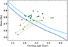 |
Fig. 1. Mass versus cooling age for currently known DAHe white dwarfs, plotted as dark green circles (with a star marking GD 356). The dark and light blue lines trace the first non-zero core crystallization fraction in hydrogen-rich white dwarfs for thin and thick envelopes, respectively (Bédard et al. 2020). The masses and effective temperatures for all stars were taken from the Gaia EDR3 white dwarf catalog (Gentile Fusillo et al. 2021). While these adopted parameters are thus consistently derived, Gaia photometry alone does not provide a robust determination of effective temperature, where intrinsic photometric variability of DAHe stars, or missing model opacities may contribute to underestimated masses and cooling ages (e.g. Reding et al. 2020; O’Brien et al. 2024). For the lowest mass points in the diagram, the light green dashed lines trace their shift in cooling age, for the case where their masses are near the minimum value for the main cluster of stars. Thus, it is plausible that all DAHe white dwarfs appear after the onset of crystallization. |
There has been limited but important prior theory on intrinsic heating mechanisms for white dwarf atmospheres. It has been proposed that acoustic and magnetohydrodynamic waves can propagate into white dwarf atmospheres. However, damping processes are strong and possibly overwhelming, implying that any detectable oscillations will be no more than a few percent in luminosity and last no longer than a few seconds (Musielak 1987; Musielak & Fontenla 1989; Musielak et al. 2005). The strong magnetic fields characteristic of the DAHe class will hinder convective motions and thus alter energy transport and structure of these stars, implying that conventional white dwarf atmospheres are unlikely to result in the observed heating. Therefore, a different mechanism of chromospheric heating is needed to account for the DAHe phenomenon.
In this work, we propose that chromospheric emission in DAHe white dwarfs is powered by Ohmic heating associated with electric currents produced by a 22Ne distillation-driven dynamo during crystallization. We argue that these stars are likely merger remnants, consistent with their systematically high masses and rotation rates. The progenitor merger events can likely enhance the 22Ne abundances in DAHe stars to the level needed to sustain strong, long-lasting dynamo action (Clayton et al. 2007; Menon et al. 2013; Shen et al. 2023). This scenario is essentially a lower-mass analogue of the 22Ne-distillation mechanism proposed to stall the cooling of ultramassive Q-branch white dwarfs (Isern et al. 1991; Segretain 1996; Blouin et al. 2021; Bédard et al. 2024; Salaris et al. 2024), and, if correct, establishes continuity between these two fascinating classes of objects. Our model and its relationship to observations are summarized in Fig. 2.
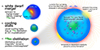 |
Fig. 2. Illustrative summary of the model advanced in this work. (a) DAHe white dwarf created by a stellar merger, such as between a carbon–oxygen and helium-core white dwarf (as shown by, e.g. Clayton et al. 2007; Menon et al. 2013) or subgiant. (b) Resulting 22Ne-rich remnant cools until the onset of carbon–oxygen crystallization and 22Ne distillation, which halt the cooling near Teff ≈ 7500 K. (c) Distillation also provides sufficient energy to sustain a strong magnetic dynamo that powers the characteristic chromospheric emission through Ohmic heating. Superscript numbers indicate observed properties of DAHe stars: 1typical masses M ≃ 0.8 M⊙, 2rapid rotation, 3similar Teff ≈ 7500 K near that of carbon–oxygen crystallization, 4magnetic fields B ≳ 5 MG, 5Balmer lines in emission, 6rotational light curve modulation, and 7lack of coronal emission in the prototype. |
This work is organized as follows. In Sect. 2, we outline our model, where the generation of magnetic fields and electric currents by a hydromagnetic dynamo is presented in Sect. 2.1, while convective motions, that provide the basic ingredients for the dynamo action, are discussed in Sect. 2.2. The magnetic field diffusion from the dynamo shell to the surface is discussed in Sect. 2.3. The dissipation of the electric currents in the atmosphere is treated in Sect. 2.4. We summarize our results, discuss immediate implications, and present considerations for future work in Sect. 3.
2. Model
2.1. Dynamo action in white dwarf interiors
One of the proposed mechanisms for the origin of white dwarf magnetic fields is a hydromagnetic dynamo that takes its energy from the convective motions produced by core crystallization. Such a dynamo is similar to that operating in the outer fluid core of the Earth, which surrounds its inner solid core, because in white dwarfs the inner crystallized core is surrounded by a convective fluid shell (Isern et al. 2017). The fast rotation observed in DAHe white dwarfs should impart a remarkable helicity to the convective flows in the outer shell because of the strong Coriolis force. Therefore, such a white dwarf dynamo is likely to be of the so-called α2 type, similar to those in the core of the Earth or in Jupiter, leading to a stationary magnetic field (Moffatt 1978).
The mean-field induction equation giving the magnetic field generated by an α2 dynamo is
 (1)
(1)
where B is the mean magnetic field, t the time, α the parameter specifying the α-effect in the dynamo, and ηt the turbulent magnetic diffusivity. The boundary conditions in the stellar dynamo are the continuity of the normal components of the magnetic field and of the current density across the boundaries of the dynamo shell, while in the case of the geodynamo, the field is assumed to be potential outside the shell because the Earth’s mantle behaves as an electric insulator (see, e.g. Glatzmaier & Roberts 1995).
While α is a tensor, for simplicity we assume it to be symmetric and isotropic, thus reducing it to a scalar. Because α is related to the helicity of the turbulent flow, it changes sign from the northern to the southern hemisphere of the star, and is a function of the latitude because the Coriolis force depends on latitude. The simplest expression one can adopt is α ∝ cos θ, where θ is the colatitude measured from the north pole. The turbulent diffusivity is also a tensor, but for the sake of simplicity, we assume it to be a scalar approximated as
 (2)
(2)
where ℓ is the characteristic length scale of the turbulent convective motions, while vt is their mean velocity (see, for example, Charbonneau 2020).
The simplest stationary mean magnetic field generated by the hydromagnetic dynamo described by Eq. (1) has the expression
 (3)
(3)
which is the expression of a force-free field with the force-free parameter β = α/ηt. Chandrasekhar (1981) showed that a non-vanishing magnetic field cannot be force-free everywhere, and thus the field must be stressed somewhere, with pressure gradients or the local gravity balancing the Lorentz force. We assume that the field is stressed at the base of the dynamo layer because the density of the fluid is larger there, and the convective velocity should not depend strongly on depth (cf. Sect. 2.2). This implies that the main field amplification process and the associated magnetic stresses are concentrated close to the base of the layer. This assumption should also be valid in the case of a non-convective dynamo, for example a Tayler–Spruit dynamo (Spruit 2002), which has recently been suggested to work during crystallization (Montgomery & Dunlap 2024).
Our dynamo magnetic field is not necessarily axisymmetric. Mean-field α2 dynamos based solely on the α effect admit non-axisymmetric dynamo solutions both in the linear and non-linear regimes, even if α is independent of the longitude (e.g. Ruediger 1980; Raedler et al. 1990; Ruediger & Elstner 1994; Moss 2005). Specifically, a linear combination of modes with degree l = 1 and azimuthal orders m = −1, 0, 1 yields a tilted dipole that can roughly describe the magnetic field of the Earth or Jupiter (Stevenson 2010, Sect. 6). We assume the same large-scale geometry can be produced in the fields of white dwarfs generated by our dynamo model, although we do not compute a full solution of Eq. (1) as a linear combination of individual dynamo modes and instead limit ourselves to the simple illustrative expression given by Eq. (3). We note that a tilted-dipole geometry is capable of accounting for the observed rotational modulation of the stellar flux (Reding et al. 2020), if the emission (or absorption) is concentrated around the poles of the field (see Sect. 2.4).
In the domain where the field is force-free, the magnetic field vector B is parallel to the electric current density J = (∇×B)/μ, where μ is the magnetic permeability of the vacuum. The parameter β is constant along each magnetic field line as can be seen by taking the divergence of both sides of Eq. (3), giving B ⋅ ∇β = 0 because ∇ ⋅ B = 0. We note, however, that β is distinct along different magnetic field lines because α and ηt are functions of the colatitude and the radial distance from the centre of the star.
An approximate expression for the order of magnitude of β can be obtained by noticing that the order of magnitude of α ∼ ℓ Ω, where Ω is the stellar spin angular velocity. Taking into account Eq. (2), we find
 (4)
(4)
which is independent of the (poorly known) mixing length ℓ. When vt goes to zero, the value of β diverges, but the electric current density, that is proportional to βB, remains finite provided that the magnetic field strength is proportional to vt. This is indeed the case when an α2-dynamo reaches equipartition between the kinetic energy density of the turbulent motions and the magnetic energy density, viz.  , where ρ is the density of the plasma.
2.2. Compositionally driven convection and the role of 22Ne distillation
The convective velocity in the dynamo fluid shell outside the crystallized core is still a subject of debate. The interior convective shell is stable to ordinary thermal convection, so convective motions are accelerated by the gradient of the molecular weight produced by oxygen crystallization. In the case of a pure carbon–oxygen mixture, solid oxygen is denser than the fluid from which it separates, and thus it sinks and forms a solid core at the centre of the star, above which the carbon–oxygen mixture remains in the liquid phase.
In recent years, the convective velocities vt associated with canonical carbon–oxygen crystallization have been steadily revised downward. Isern et al. (2017) first derived an upper limit ≈35 km s−1, but this was later refined downward to ≃1 m s−1 by Ginzburg et al. (2022) when considering the mixing of buoyantly rising material, and even further by Fuentes et al. (2023) when accounting for the stabilizing effect of the thermal stratification. In white dwarfs with a rotation period of the order of one hour, the Coriolis force increases the velocity of the compositional convection in the regime considered by Fuentes et al. (2023), but even in that case the velocity does not exceed 10−4 m s−1 (see Montgomery & Dunlap 2024, for a similar conclusion). Owing to the large dimensions of the convective eddies (comparable with the pressure scale height ∼106 m) and the small magnetic diffusivity in a degenerate plasma, the dynamo number is still supercritical and dynamo action can occur. However, the generated magnetic field strengths are at most of the order of several hundred of gauss, orders of magnitude smaller than required to account for the observations. This happens even when we assume that the Lorentz force reaches equipartition with the Coriolis force, as expected in fast-rotating, highly supercritical α2 dynamos, because the convective velocity is extremely small (cf. Sect. 3.2 of Ginzburg et al. 2022).
Furthermore, while a dynamo generated by the onset of crystallization may be able to produce the 1 − 100 MG fields characteristic of magnetic white dwarfs (Castro-Tapia et al. 2024; Fuentes et al. 2024), the associated convection is only sufficient for a small fraction of a white dwarf lifetime (∼10 Myr for M = 0.9 M⊙). It is therefore unlikely to power the chromospheric emission in DAHe stars, which may represent ≈14% of magnetic white dwarfs at the relevant Teff (Manser et al. 2023). If DAHe stars are merger remnants, a merger-driven dynamo may also produce a strong field (Schneider et al. 2019), but would not result in a lasting dynamo which could power the chromosphere.
To overcome the low velocities predicted by the model of Fuentes et al. (2023) for the case of compositional convection, we conjecture that motions associated with the distillation of 22Ne (originally proposed by Isern et al. 1991) can produce sufficiently fast flows. To be more specific, we consider the case of a white dwarf with central composition mass-fractions X(16O) = 0.6, X(12C) = 0.365, and X(22Ne) = 0.035 (case (a) discussed by Blouin et al. 2021). Such a 22Ne-rich composition is possible when the progenitor of a carbon–oxygen white dwarf formed in a particularly α-rich environment or when it resulted from a merger (see Clayton et al. 2007; Menon et al. 2013; Shen et al. 2023; Salaris et al. 2024), where corresponding evolutionary models have largely reproduced the overdensity of stars in the Q branch of the white dwarf HR diagram (cf. Tremblay et al. 2019; Cheng et al. 2019; Bédard et al. 2024). Indeed, the relatively high mass and fast rotation that characterize DAHe stars can be easily accounted for if they are merger remnants. In our model, it is assumed the conditions for 22Ne distillation are met, and leave detailed studies of specific merger scenarios to future work.
We estimate the size and the rising velocity of the solid flakes formed by the 22Ne distillation in Appendix A, finding these to be of the order of 10−4 m and (5 − 10) m s−1, respectively. During its rise, a solid flake produces a turbulent wake that extends across the full vertical depth it spans. The slow diffusion of these turbulent wakes under the action of the small kinematic viscosity ν in a white dwarf interior (ν ∼ 3 × 10⁻⁶ m2 s−1; Isern et al. 2017) produces a turbulent velocity field remarkably faster than that due to the compositional convection alone.
The mean-field dynamo equations (Moffatt 1978; Charbonneau 2020) can be non-dimensionalized with different choices for the unit of length. Here, we propose that the appropriate length scale is ζlw instead of the star radius, where ζ is the volume filling factor of the flake turbulent wakes and lw is their average vertical extension. The value of lw ∼ (|Δρ|/ρ)Hρ, where Hρ ∼ 3 × 10⁶ m is the density scale height at the surface of the core of a 0.9 M⊙ white dwarf (cf. Fuentes et al. 2024, table 1). Therefore, we conjecture that the dynamo number can be defined as D = ζαlw/ηt. Considering a white dwarf with Ω = 10−3 s−1, a conservative turbulent velocity vt ∼ 1 m s−1, and a length of the wakes of lw ∼ 3 × 10⁵ m, we find a supercritical dynamo number D ∼ 10 for a volume filling factor ζ ∼ 0.03. The geometry of the most easily excited magnetic field mode is that of a dipole with a length scale comparable with the star radius (cf. Raedler et al. 1990, Table 1). In such a dynamo, the magnetic field strength attained when the Lorentz force reaches equipartition with the Coriolis force is of the order of 10 MG for a rotation period of 1 h and turbulent velocities of ∼1 m s−1 (cf. Sect. 3.2 of Ginzburg et al. 2022).
2.3. Diffusion of the magnetic field to the stellar surface
In our simplified model, the mean field is force-free, that is, the Lorentz force vanishes. Therefore, the magnetic field does not affect the white dwarf equilibrium structure and stratification, which are instead set by a balance between pressure and gravity only. This is also true in the outer layers of the white dwarf, if the surface field is sufficiently strong (roughly MG) to halt near-surface convection. The vanishing Lorentz force also implies that magnetohydrodynamic forces such as magnetic pressure or magnetic buoyancy cannot bring magnetic fields to the surface (as in the Sun or sunlike stars). The strong field also quenches any plasma flow, thus preventing any transport by advection. Only magnetic diffusion can transport the field from the dynamo region to the stellar surface.
Ginzburg et al. (2022) computed the magnetic diffusion timescale for two white dwarfs of masses 0.6 and 0.8 M⊙ finding that it becomes drastically reduced when the convection zone reaches the lower boundary of the helium envelope. At that point, the diffusion time from the dynamo shell to the atmosphere becomes of the order 0.1 Gyr for 0.8 M⊙, and 1 Gyr for 0.6 M⊙. A more detailed analysis by Blatman & Ginzburg (2024) confirms such timescales, predicting a diffusion timescale of ∼0.6 Gyr shortly after the field breaks out at the surface of a 0.8 M⊙ white dwarf, which occurs when the star has a cooling age of ∼3 Gyr.
An analysis of the diffusion is presented in Appendix B, where we show that the field remains approximately force-free during the process. In such a regime, the field and the associated currents flowing along the field lines diffuse to the surface of the star reaching its photosphere. Those photospheric currents are responsible for the DAHe phenomenology because they produce a strong Ohmic heating in the atmosphere (cf. Sect. 2.4).
Crucially, the magnetic field lines remain connected to the dynamo shell throughout the process of diffusing. As a consequence, the value of the force-free parameter β along each magnetic field line in the stellar atmosphere is set inside the dynamo region, because the force-free regime extends from the top of the dynamo shell to the atmosphere of the star. The disconnection of the surface field from the dynamo region can occur only on the global diffusion timescale of the field itself, that is, on the order of 10 Gyr, owing to its large spatial scale, L, that is comparable with the stellar radius. In a white dwarf of 0.8 M⊙, the thickness of the layer separating the convection zone from the surface, ds ∼ 0.2 Rs < L, and becomes shorter as the star cools (cf. Fig. 1 of Blatman & Ginzburg 2024).
Our scenario aims to reproduce a steady atmospheric heating consistent with observations of the DAHe phenomenon. It therefore requires that the force-free fields generated by the dynamo are stable. Unstable fields would be destroyed on the Alfvén timescale. Molodensky (1974) found that force-free fields are stable to perturbations both in the photosphere (due to the expected small-scale motions, e.g. Tremblay et al. 2015) as well as above the photosphere (such as those produced by hydromagnetic waves) as long as the typical length scale of such perturbations lpert ≪ β−1. Because β−1 > ds ∼ 0.2 Rs corresponds to the length scale of a global field in the present regime, this condition is certainly satisfied (see Sect. 2.4 for a realistic estimate of β). It is interesting to note that small scale photospheric motions can lead to the formation of tangential discontinuities in the atmospheric magnetic fields that are sites of strong current concentration and heating by Ohmic dissipation (see Low 2023, for a recent review).
2.4. Chromospheric heating power estimate
In the absence of external energy sources, electric currents flowing parallel to the field in the atmosphere produce a steady dissipation of magnetic energy until the field reaches a potential configuration with β = 0 after which there is no further dissipation (cf. Eq. (5)). However, even in the presence of strong atmospheric dissipation, such a potential field state cannot be fully reached while the hydromagnetic dynamo is in operation and the field lines remain connected with the dynamo shell. In this regime, the dissipated electric energy is ultimately provided by the interior dynamo.
To calibrate our subsequent estimates, we supply some characteristic scales in this problem. For the DAHe prototype GD 356, Rs = 0.01 R⊙, Ω ∼ 10−3 s−1, and B ∼ 10 MG. This radius is representative of carbon–oxygen white dwarfs in general, but the rotation rates of DAHe stars lie in the range 10−4–10−2 s−1. While the field strengths of DAHe stars are not tightly constrained (only GD 356 has been monitored through its rotational cycle), they are estimated to be between 5 and 50 MG (Manser et al. 2023), consistent with a disc-averaged mean field ∼10 MG. The convective velocity vt is estimated to be vt ∼ 5 − 10 m s−1 (see Sect. 2.2).
The dissipation per unit volume can be computed from the induction equation assuming that no motion occurs in the atmospheric plasma, so that
 (5)
(5)
where η is the microscopic magnetic diffusivity in the atmosphere (Spitzer 1962), since turbulence and convection are strongly suppressed by the magnetic field (e.g. Saumon et al. 2022).
The magnetic diffusivity in the non-degenerate plasma of the stellar atmosphere is given by the usual Spitzer expression (e.g. Meyer et al. 1974)
 (6)
(6)
where T is the plasma temperature in Kelvin. We discuss the suitability of such an expression in Appendix C. The greatest dissipation is reached in the atmosphere where T is minimum. In the case of GD 356 and DAHe white dwarfs, T ≈ 7500 K, so that η ≈ 460 m2 s−1.
Taking the scalar product of Eq. (5) by B and making use of the relationship for two generic vector fields u and w, ∇ ⋅ (u × w) = w ⋅ (∇×u)−u ⋅ (∇×w), we obtain
![Mathematical equation: $$ \begin{aligned} {\boldsymbol{B}} \cdot \frac{\partial {\boldsymbol{B}}}{\partial t} = \nabla \cdot \left[ \eta {\boldsymbol{B}} \times (\nabla \times {\boldsymbol{B}}) \right] - \eta (\nabla \times {\boldsymbol{B}})^{2}, \end{aligned} $$](/articles/aa/full_html/2024/09/aa49947-24/aa49947-24-eq8.gif) (7)
(7)
which can be reduced to
 (8)
(8)
where we made use of the force-free configuration of the field B (cf. Eq. (3)) to eliminate the first term on the right-hand side of Eq. (7).
During the period of time when the magnetic field has not yet diffused to the surface, β is given by Eq. (4). However, once the field has broken through, efficient Ohmic dissipation in the atmosphere globally affects the dynamo field as a boundary condition. At this time (corresponding to the onset of the DAHe phenomenon), atmospheric diffusion modifies β along an entire field line and sets the value of the current dissipation rate in the photosphere.
As soon as the magnetic field reaches the surface, the values of β characterizing the field are modified essentially instantaneously. To see this, we recast Eq. (8) in the simpler form (making use of Eq. (3)):
 (9)
(9)
For the initial values of β given by Eq. (4),
 (10)
(10)
Ohmic dissipation therefore quickly relaxes the global field on a timescale
 (11)
(11)
when assuming a dynamo convective velocity vt ∼ 10 m s−1, η = 460 m2 s−1, and Ω = 10−3 s−1.
We argue that the resistive heating power experienced by the chromosphere is set by the rate at which the dynamo can amplify the magnetic field. The associated timescale is comparable to the diffusion timescale
 (12)
(12)
across the dynamo region, with extent Ldyn ≲ Rs (Brandenburg 2001). In other words, Pdiss is ultimately limited by the rate at which the dynamo can replenish the non-potential component of the field in the first place.
Pdiss can be found by integrating B2/(2μτdiss) over the atmosphere. The pressure scale height in the atmosphere of a white dwarf with effective temperature 7500 K is h ∼ 100 m, while the density near the photosphere (optical depth τ ∼ 1 for λ ≈ 5000 Å) is approximately 10−2 kg m−3 (e.g. Saumon et al. 2022). Roughly estimating that the Hα line forms over an isothermal region of vertical extent H ∼ 10h ∼ 1 km above the photosphere, the density at the top of the chromosphere is ≈4.5 × 10⁻⁷ kg m−3, comparable with the density of the solar photosphere at its temperature minimum.
Assuming Ldyn ≳ 3 × 10⁶ m, lw ∼ 3 × 10⁵ m, and vt ∼ 5 − 10 m s−1 (to estimate ηt through Eq. (2)), we find that τheat ∼ τdiff ≳ 107 s. Finally, this implies a heating rate
 (13)
(13)
corresponding to a value of β ∼ 10−8 m .
.
We notice that the dissipation follows the latitudinal dependence of the α effect, which is concentrated toward the high latitudes, while it vanishes at the equator where α changes sign (cf. Eq. (4)). Therefore, in our simple model, the power dissipated per unit surface area varies with the colatitude proportionally to cos2θ and is maximum at the poles. An examination of available DAHe spectra demonstrates that the ±σ components of Hα do not exhibit splitting variations consistent with those expected for a magnetic dipole. Such changes would be on the order of 20% because the observable field is integrated over the visible hemisphere, which averages the factor-of-two changes from pole to equator in a magnetic dipole. However, only GD 356 has data with full spin phase coverage, showing that its line splitting, coming from the integrated field of the visible hemisphere, hardly varies with rotation.
Three other DAHe stars show stronger variations, providing information about the distribution of field strength and emission regions over their surfaces. These are SDSS J1252−0234 (Reding et al. 2020), whose emission lines diminish into an absorption feature, then reappear as the star rotates; SDSS J1219+4715 (Gänsicke et al. 2020), whose emission strength varies, but not field strength; and WD J1616+5410 (Manser et al. 2023), for which emission strength and field strength may vary. These data indicate that the emission region does not fully cover the star and is likely concentrated in a patch (Ferrario et al. 1997). Also, the fields revealed in emission generally do not seem to show much broadening in their σ components, which hints that, except for WD J1616+5410, the field strength in the emission regions may be uniform. Altogether, these observations may indicate that the assumption of a dipolar field could be a convenient simplification from a theoretical point of view, but not necessarily in agreement with observations. Detailed models for these DAHe stars, from repeated spectropolarimetric measurements made through their rotation cycles, could provide insights into the validity of this model.
Our proposed mechanism is consistent with the lack of coronal and transition region emission in DAHe stars. To generate a corona, it is necessary to dissipate electric currents at high temperatures of the order of 106 K. However, an effective dissipation at temperatures of ∼106 K is forbidden by the dramatic decrease in the magnetic diffusivity η ∝ T−3/2, which becomes ∼10−3 − 10−4 times smaller than in the chromosphere. The rapid decrease of the electric resistivity with temperature serves as a “thermostat” which keeps most of the atmospheric plasma at ∼104 K. We note that any plasma at ∼105 K (typical of the solar or stellar transition regions) is mainly heated by conduction from a hotter overlying corona, so we do not expect to observe extreme ultraviolet line emission if a corona is absent. Furthermore, DAHe stars should have pure hydrogen atmospheres and thus lack any atomic transitions beyond the Lyman series.
3. Summary, implications, and future work
We have proposed that Ohmic heating from dynamo-driven currents is responsible for the DAHe phenomenon, ultimately caused by carbon–oxygen crystallization and distillation of 22Ne. We argue that the high concentrations of 22Ne needed to drive the required dynamo can be naturally accounted for if DAHe white dwarfs are merger remnants. In this picture, DAHe stars may be a lower-mass analogue of ultramassive Q branch white dwarfs whose observed cooling delays are likely also caused by 22Ne distillation. However, we refrain from advocating a particular merger scenario for creating the required 22Ne abundances.
The main points of the DAHe white dwarf modeling can be summarized as follows:
-
(i)
22Ne distillation drives dynamos that result in strong magnetic fields.
-
(ii)
Atmospheric heating is maximal at the magnetic poles, and zero at the equator.
-
(iii)
Coronae are never produced owing to the temperature dependence of the resistivity.
-
(iv)
Misaligned magnetic and spin axes will cause the chromospheric regions to rotate in and out of view.
-
(v)
A merger origin that enhances 22Ne is consistent with their relatively high masses and fast spins.
-
(vi)
22Ne distillation should facilitate a cooling delay, consistent with the observed clustering in the HR diagram.
The mechanism in this work requires a relatively high 22Ne abundance, but is agnostic as to its origin. A merger scenario has been invoked to address the overdensity of Q branch white dwarfs (e.g., Shen et al. 2023; Bédard et al. 2024), and merits further investigation in the context of the DAHe phenomenon. Depending on the specific merger scenario, it might be expected that DAHe stars lack close, unevolved companions, similar to isolated magnetic white dwarfs suspected to have similar origins (Liebert et al. 2005; Tout et al. 2008; García-Berro et al. 2012).
Furthermore, a key corollary of this model is that white dwarfs on the Q branch that distill 22Ne should also be magnetic and produce chromospheres. Notably, there are two massive DQe white dwarfs known, both of which have emission lines detected only in the ultraviolet: both G227-5 and G35-26 exhibit emission lines of C II and O I, where the latter star shows additional emission species (e.g. N I, Mg II, Si IIProvencal et al. 2005). While neither star is currently known to be magnetic, hot DQ stars as a population are suspected stellar mergers (Dunlap & Clemens 2015; Coutu et al. 2019), and possibly consistent with belonging to the delayed cooling population of the Q branch. A modest number of hot DQ stars have been reported to be magnetic, fast rotators, but definitive studies and interpretations are lacking (Dufour et al. 2013; Lawrie et al. 2013; Williams et al. 2016). As predicted, the two aforementioned DQe stars lie within the Q branch of the HR diagram.
One implication of our model is that DAHe white dwarfs should experience substantial cooling delays for many gigayears, depending on the abundance of 22Ne in their cores (Camisassa et al. 2021; Blouin et al. 2021; Bédard et al. 2024). While one might expect to find some ancient DAHe stars based on kinematics, the known members are a thin disk population with ⟨vtan⟩ = 27 ± 13 km s−1. From an observational perspective, this is a direct consequence of the Gaia magnitude limit, and the shared MG = 13.2 mag of the DAHe population, restricting their detection to within roughly 150 pc, where thick disc and halo stars are rare (Bensby et al. 2014; Zubiaur et al. 2024). From a theoretical viewpoint, any thick disc or halo mergers may have insufficient metallicities to produce the 22Ne necessary for distillation and stalled cooling (Salaris et al. 2024). It is therefore possible that few high-velocity members will be found among DAHe white dwarfs, at least until a sufficiently large sample is available.
An interesting point to address in future investigations is the interaction between the atmospheric currents considered in the present model and hydromagnetic waves that can propagate along the same field lines (e.g. Musielak et al. 2005). Such waves can be excited in the atmospheres of DAHe stars, because motions are still allowed along magnetic field lines (cf. Tremblay et al. 2015), and such motions will produce magneto-acoustic waves whose propagation will not be confined to the field lines. Such waves may produce shocks, heating the local atmosphere effectively. Moreover, not all horizontal motions will be suppressed–some may survive and excite Alfvén waves which, although difficult to damp, can couple to magneto-acoustic waves and contribute to heating. Radiative damping effects, which are strong for pure acoustic waves in white dwarf atmospheres, would be significantly reduced for magneto-acoustic waves. On the other hand, they are absent for Alfvén waves because they are purely transverse magnetic modes that produce no heating of the plasma by compression. Therefore, the propagation of Alfvén waves cannot directly modify the plasma radiation.
Several aspects of the model we have introduced are addressed in a mainly qualitative way, although making use of the results of previous quantitative studies of stellar dynamos. A quantitative, mean field dynamo model based on numerical calculations can represent the next step of an investigation. Another topic to be addressed in future investigations is the inclusion of the proposed Ohmic heating in radiative transfer models of white dwarf atmospheres in order to provide quantitative predictions of the expected fluxes both in the continuum and in the spectral lines. Those predictions will hopefully allow a detailed test of the model proposed in the present study by means of a quantitative comparison with the observations.
A degenerate star spectrum (D), with Balmer lines strongest (A), Zeeman-split (H), and in emission (e).
Acknowledgments
The authors gratefully acknowledge an insightful and inspiring report by the referee, J. Isern, who suggested to explore the 22Ne distillation as a potential source of energy to generate turbulent motions in white dwarfs. Moreover, the authors acknowledge highly valuable conversations and ideas shared by Z. E. Musielak and M. R Schreiber. They are also grateful to J. Fuller for useful comments, and to A. Bédard and M. Hollands for clarifications on evolutionary model grids. This research was supported by the Munich Institute for Astro-, Particle and BioPhysics (MIAPbP) which is funded by the Deutsche Forschungsgemeinschaft under Germany’s Excellence Strategy EXC 2094−390783311. AFL gratefully acknowledges support from the 2023 INAF Program for Fundamental Astrophysics through the project entitled “Unveiling the magnetic side of stars” (P.I. Dr. A. Bonanno) and from the European Union – NextGenerationEU RRF M4C2 1.1 n: 2022HY2NSX project “CHRONOS: adjusting the clock(s) to unveil the CHRONO-chemo-dynamical Structure of the Galaxy” (PI: Dr. S. Cassisi). NZR acknowledges support from the National Science Foundation Graduate Research Fellowship under Grant No. DGE–1745301.
References
- Amorim, L. L., Kepler, S. O., Külebi, B., Jordan, S., & Romero, A. D. 2023, ApJ, 944, 56 [NASA ADS] [CrossRef] [Google Scholar]
- Angel, J. R. P., & Landstreet, J. D. 1971, ApJ, 164, L15 [NASA ADS] [CrossRef] [Google Scholar]
- Bagnulo, S., & Landstreet, J. D. 2021, MNRAS, 507, 5902 [NASA ADS] [CrossRef] [Google Scholar]
- Bagnulo, S., & Landstreet, J. D. 2022, ApJ, 935, L12 [NASA ADS] [CrossRef] [Google Scholar]
- Bédard, A., Bergeron, P., Brassard, P., & Fontaine, G. 2020, ApJ, 901, 93 [Google Scholar]
- Bédard, A., Blouin, S., & Cheng, S. 2024, Nature, 627, 286 [CrossRef] [Google Scholar]
- Bensby, T., Feltzing, S., & Oey, M. S. 2014, A&A, 562, A71 [NASA ADS] [CrossRef] [EDP Sciences] [Google Scholar]
- Blatman, D., & Ginzburg, S. 2024, MNRAS, 528, 3153 [NASA ADS] [CrossRef] [Google Scholar]
- Blouin, S., Daligault, J., & Saumon, D. 2021, ApJ, 911, L5 [NASA ADS] [CrossRef] [Google Scholar]
- Brandenburg, A. 2001, ApJ, 550, 824 [Google Scholar]
- Camisassa, M. E., Althaus, L. G., Torres, S., et al. 2021, A&A, 649, L7 [NASA ADS] [CrossRef] [EDP Sciences] [Google Scholar]
- Cassisi, S., Potekhin, A. Y., Pietrinferni, A., Catelan, M., & Salaris, M. 2007, ApJ, 661, 1094 [NASA ADS] [CrossRef] [Google Scholar]
- Castro-Tapia, M., Cumming, A., & Fuentes, J. R. 2024, ApJ, 969, 10 [NASA ADS] [CrossRef] [Google Scholar]
- Chandrasekhar, S. 1981, Hydrodynamic and Hydromagnetic Stability, Dover Books on Physics Series (Dover Publications) [Google Scholar]
- Charbonneau, P. 2020, Liv. Rev. Sol. Phys., 17, 4 [Google Scholar]
- Cheng, S., Cummings, J. D., & Ménard, B. 2019, ApJ, 886, 100 [Google Scholar]
- Clayton, G. C., Geballe, T. R., Herwig, F., Fryer, C., & Asplund, M. 2007, ApJ, 662, 1220 [NASA ADS] [CrossRef] [Google Scholar]
- Coutu, S., Dufour, P., Bergeron, P., et al. 2019, ApJ, 885, 74 [NASA ADS] [CrossRef] [Google Scholar]
- Dufour, P., Vornanen, T., Bergeron, P., Fontaine, Berdyugin A., 2013, ASP Conf. Ser., 469, 167 [NASA ADS] [Google Scholar]
- Dunlap, B. H., & Clemens, J. C. 2015, ASP Conf. Ser., 493, 547 [NASA ADS] [Google Scholar]
- Farihi, J., Hermes, J. J., Littlefair, S. P., et al. 2023, MNRAS, 525, 1097 [NASA ADS] [CrossRef] [Google Scholar]
- Ferrario, L., Wickramasinghe, D. T., Liebert, J., Schmidt, G. D., & Bieging, J. H. 1997, MNRAS, 289, 105 [NASA ADS] [CrossRef] [Google Scholar]
- Ferrario, L., de Martino, D., & Gänsicke, B. T. 2015, Space Sci. Rev., 191, 111 [Google Scholar]
- Fuentes, J. R., Cumming, A., Castro-Tapia, M., & Anders, E. H. 2023, ApJ, 950, 73 [NASA ADS] [CrossRef] [Google Scholar]
- Fuentes, J. R., Castro-Tapia, M., & Cumming, A. 2024, ApJ, 964, L15 [NASA ADS] [CrossRef] [Google Scholar]
- Gänsicke, B. T., Rodríguez-Gil, P., Gentile Fusillo, N. P., et al. 2020, MNRAS, 499, 2564 [CrossRef] [Google Scholar]
- García-Berro, E., Lorén-Aguilar, P., Aznar-Siguán, G., et al. 2012, ApJ, 749, 25 [CrossRef] [Google Scholar]
- Gentile Fusillo, N. P., Tremblay, P. E., Cukanovaite, E., et al. 2021, MNRAS, 508, 3877 [NASA ADS] [CrossRef] [Google Scholar]
- Ginzburg, S., Fuller, J., Kawka, A., & Caiazzo, I. 2022, MNRAS, 514, 4111 [NASA ADS] [CrossRef] [Google Scholar]
- Glatzmaier, G. A., & Roberts, P. H. 1995, Nature, 377, 203 [CrossRef] [Google Scholar]
- Goldreich, P., & Lynden-Bell, D. 1969, ApJ, 156, 59 [Google Scholar]
- Greenstein, J. L., & McCarthy, J. K. 1985, ApJ, 289, 732 [CrossRef] [Google Scholar]
- Hardy, F., Dufour, P., & Jordan, S. 2023, MNRAS, 520, 6111 [CrossRef] [Google Scholar]
- Hubbard, W. B., & Lampe, M. 1969, ApJS, 18, 297 [NASA ADS] [CrossRef] [Google Scholar]
- Isern, J., Hernanz, M., Mochkovitch, R., & Garcia-Berro, E. 1991, A&A, 241, L29 [NASA ADS] [Google Scholar]
- Isern, J., García-Berro, E., Külebi, B., & Lorén-Aguilar, P. 2017, ApJ, 836, L28 [NASA ADS] [CrossRef] [Google Scholar]
- Itoh, N., Uchida, S., Sakamoto, Y., Kohyama, Y., & Nozawa, S. 2008, ApJ, 677, 495 [NASA ADS] [CrossRef] [Google Scholar]
- Kavanagh, R. D., & Vedantham, H. K. 2023, MNRAS, 524, 6267 [NASA ADS] [CrossRef] [Google Scholar]
- Kemp, J. C., Swedlund, J. B., Landstreet, J. D., & Angel, J. R. P. 1970, ApJ, 161, L77 [NASA ADS] [CrossRef] [Google Scholar]
- Kilic, M., Moss, A. G., Kosakowski, A., et al. 2023, MNRAS, 518, 2341 [Google Scholar]
- Kippenhahn, R., Weigert, A., & Weiss, A. 2013, Stellar Structure and Evolution (Berlin: Springer) [Google Scholar]
- Lanza, A. F. 2013, A&A, 557, A31 [NASA ADS] [CrossRef] [EDP Sciences] [Google Scholar]
- Lawrie, K. A., Burleigh, M. R., Dufour, P., & Hodgkin, S. T. 2013, MNRAS, 433, 1599 [NASA ADS] [CrossRef] [Google Scholar]
- Li, J., Ferrario, L., & Wickramasinghe, D. 1998, ApJ, 503, L151 [NASA ADS] [CrossRef] [Google Scholar]
- Liebert, J., Wickramasinghe, D. T., Schmidt, G. D., et al. 2005, AJ, 129, 2376 [NASA ADS] [CrossRef] [Google Scholar]
- Low, B. C. 2023, Phys. Plasmas, 30, 012903 [NASA ADS] [CrossRef] [Google Scholar]
- Manser, C. J., Gänsicke, B. T., Inight, K., et al. 2023, MNRAS, 521, 4976 [NASA ADS] [CrossRef] [Google Scholar]
- Menon, A., Herwig, F., Denissenkov, P. A., et al. 2013, ApJ, 772, 59 [NASA ADS] [CrossRef] [Google Scholar]
- Meyer, F., Schmidt, H. U., Weiss, N. O., & Wilson, P. R. 1974, MNRAS, 169, 35 [Google Scholar]
- Mochkovitch, R. 1983, A&A, 122, 212 [NASA ADS] [Google Scholar]
- Moffatt, H. K. 1978, Magnetic Field Generation in Electrically Conducting Fluids, Cambridge Monographs on Mechanics (Cambridge University Press) [Google Scholar]
- Molodensky, M. M. 1974, Sol. Phys., 39, 393 [CrossRef] [Google Scholar]
- Montgomery, M. H., & Dunlap, B. H. 2024, ApJ, 961, 197 [NASA ADS] [CrossRef] [Google Scholar]
- Moss, D. 2005, A&A, 432, 249 [NASA ADS] [CrossRef] [EDP Sciences] [Google Scholar]
- Musielak, Z. E. 1987, ApJ, 322, 234 [NASA ADS] [CrossRef] [Google Scholar]
- Musielak, Z. E., & Fontenla, J. M. 1989, ApJ, 346, 435 [NASA ADS] [CrossRef] [Google Scholar]
- Musielak, Z. E., Winget, D. E., & Montgomery, M. H. 2005, ApJ, 630, 506 [NASA ADS] [CrossRef] [Google Scholar]
- Nandkumar, R., & Pethick, C. J. 1984, MNRAS, 209, 511 [NASA ADS] [CrossRef] [Google Scholar]
- O’Brien, M. W., Tremblay, P. E., Klein, B. L., et al. 2024, MNRAS, 527, 8687 [Google Scholar]
- Piddington, J. H., & Drake, J. F. 1968, Nature, 217, 935 [NASA ADS] [CrossRef] [Google Scholar]
- Priest, E. 1984, Solar Magnetohydrodynamics, Geophysics and Astrophysics Monographs (Netherlands: Springer) [Google Scholar]
- Provencal, J. L., Shipman, H. L., & MacDonald, J. 2005, ApJ, 627, 418 [NASA ADS] [CrossRef] [Google Scholar]
- Raedler, K. H., Wiedemann, E., Brandenburg, A., Meinel, R., & Tuominen, I. 1990, A&A, 239, 413 [NASA ADS] [Google Scholar]
- Reding, J. S., Hermes, J. J., Vanderbosch, Z., et al. 2020, ApJ, 894, 19 [NASA ADS] [CrossRef] [Google Scholar]
- Reding, J. S., Hermes, J. J., Clemens, J. C., Hegedus, R. J., & Kaiser, B. C. 2023, MNRAS, 522, 693 [NASA ADS] [CrossRef] [Google Scholar]
- Ruediger, G. 1980, Astron. Nachr., 301, 181 [NASA ADS] [CrossRef] [Google Scholar]
- Ruediger, G., & Elstner, D. 1994, A&A, 281, 46 [Google Scholar]
- Salaris, M., Blouin, S., Cassisi, S., & Bedin, L. R. 2024, A&A, 686, A153 [NASA ADS] [CrossRef] [EDP Sciences] [Google Scholar]
- Saumon, D., Blouin, S., & Tremblay, P.-E. 2022, Phys. Rep., 988, 1 [NASA ADS] [CrossRef] [Google Scholar]
- Schneider, F. R., Ohlmann, S. T., Podsiadlowski, P., et al. 2019, Nature, 574, 211 [CrossRef] [Google Scholar]
- Segretain, L. 1996, A&A, 310, 485 [NASA ADS] [Google Scholar]
- Shen, K. J., Blouin, S., & Breivik, K. 2023, ApJ, 955, L33 [NASA ADS] [CrossRef] [Google Scholar]
- Spitzer, L. 1962, Physics of Fully Ionized Gases (Interscience New York) [Google Scholar]
- Spruit, H. C. 2002, A&A, 381, 923 [CrossRef] [EDP Sciences] [Google Scholar]
- Stevenson, D. J. 2010, Space Sci. Rev., 152, 651 [NASA ADS] [CrossRef] [Google Scholar]
- Tout, C. A., Wickramasinghe, D. T., Liebert, J., Ferrario, L., & Pringle, J. E. 2008, MNRAS, 387, 897 [NASA ADS] [CrossRef] [Google Scholar]
- Tremblay, P. E., Fontaine, G., Freytag, B., et al. 2015, ApJ, 812, 19 [Google Scholar]
- Tremblay, P.-E., Fontaine, G., Gentile Fusillo, N. P., et al. 2019, Nature, 565, 202 [CrossRef] [Google Scholar]
- Walters, N., Farihi, J., Marsh, T. R., et al. 2021, MNRAS, 503, 3743 [NASA ADS] [CrossRef] [Google Scholar]
- Weisskopf, M. C., Wu, K., Trimble, V., et al. 2007, ApJ, 657, 1026 [Google Scholar]
- Wickramasinghe, D. T., Farihi, J., Tout, C. A., Ferrario, L., & Stancliffe, R. J. 2010, MNRAS, 404, 1984 [NASA ADS] [Google Scholar]
- Williams, K. A., Montgomery, M. H., Winget, D. E., Falcon, R. E., & Bierwagen, M. 2016, ApJ, 817, 27 [Google Scholar]
- Zarka, P. 2007, Planet. Space Sci., 55, 598 [Google Scholar]
- Zubiaur, Ainhoa, Raddi, Roberto, & Torres, Santiago 2024, A&A, 687, A286 [NASA ADS] [CrossRef] [EDP Sciences] [Google Scholar]
Appendix A: Size and velocity of buoyant flakes
When white dwarfs reach a central temperature equal to that of the crystallization phase transition, the formation of buoyant oxygen-rich crystals depleted of 22Ne occurs at their centres (cf. Isern et al. 1991; Blouin et al. 2021). The formation of solid flakes requires the diffusion of the crystallization latent heat to allow the fluid to become solid. If we indicate the size of a flake with f, the timescale for heat diffusion is th ∼ f2/λ, where λ is the thermal diffusivity. If a flake ascends with a terminal velocity vf, its characteristic dynamical timescale is of the order of tdyn ∼ 2f/vf. We assume that the size of a flake and its terminal velocity are constrained by th ∼ tdyn that gives the equation
 (A.1)
(A.1)
The terminal velocity vf was estimated by Mochkovitch (1983) assuming the Stokes law, that is valid for a Reynolds number of order unity. As a matter of fact, it will be shown that the Reynolds number is remarkably larger than the unity, so we adopt the aerodynamic drag to describe the interaction between a rising flake and the surrounding fluid. By equating the drag to the buoyancy acting on a flake, we obtain its terminal velocity as
![Mathematical equation: $$ \begin{aligned} v_{\rm f} \sim \left[ C_{\rm D}^{-1} f g \left( \frac{\Delta \rho }{\rho } \right) \right]^{1/2}, \end{aligned} $$](/articles/aa/full_html/2024/09/aa49947-24/aa49947-24-eq17.gif) (A.2)
(A.2)
where CD is the coefficient of aerodynamic drag that we assume to be unity for simplicity, g is the acceleration of gravity, and Δρ/ρ is the relative density difference between a solid flake and the surrounding fluid (in absolute value), which we take to be in the range 0.01–0.1 (see Blouin et al. 2021, Fig. 2). Making use of Eqs. (A.1) and (A.2), we obtain
![Mathematical equation: $$ \begin{aligned} f \sim (2\lambda )^{2/3} \left[ g \left(\frac{\Delta \rho }{\rho } \right) \right]^{-1/3} \end{aligned} $$](/articles/aa/full_html/2024/09/aa49947-24/aa49947-24-eq18.gif) (A.3)
(A.3)
and
![Mathematical equation: $$ \begin{aligned} v_{\rm f} \sim \left[ f g \left( \frac{\Delta \rho }{\rho }\right)\right]^{1/2}. \end{aligned} $$](/articles/aa/full_html/2024/09/aa49947-24/aa49947-24-eq19.gif) (A.4)
(A.4)
The thermal diffusivity λ is a function of the electron thermal conductivity κcond (Hubbard & Lampe 1969; Cassisi et al. 2007) according to
 (A.5)
(A.5)
where ρ is the plasma density and cp is the specific heat at constant pressure that we assume to be approximately equal to 3kb per unit particle, where kb is the Boltzmann constant, an expression appropriate at solidification neglecting the contribution of the electrons that is ≈25% of that of the ions (cf. Sect. 37.3 of Kippenhahn et al. 2013). Given that this treatment is only a rough approximation, we do not increase its uncertainty if we compute κcond from its ratio to the electric conductivity, that is a simple function of the temperature (cf. Itoh et al. 2008), and adopt the electric conductivity for the interior of a white dwarf as estimated by Isern et al. (2017). With this simplification, we obtain λ ∼ 10−3 m2 s−1 for a solidification temperature of 6 × 10⁶ K as given by Castro-Tapia et al. (2024) for a white dwarf mass of 0.8 M⊙. For an acceleration of gravity g = 107 m s−2, from Eqs. (A.3) and (A.4), we obtain f ∼ (1.6 − 3.5)×10−4 m and vf ∼ (6 − 12) m s−1. The Reynolds number is  for a kinematic viscosity ν ∼ 3 × 10⁻⁶ m2 s−1 as estimated by Isern et al. (2017) and is independent of Δρ/ρ. A posteriori, such a value justifies the adoption of the aerodynamic drag formula instead of the Stokes formula. More importantly, it indicates that the wake past a rising solid flake is turbulent, thus providing a turbulent velocity field much faster than predicted by compositional convection according to Fuentes et al. (2023).
Appendix B: Diffusion of the magnetic field
Considering Eq. (5), and that the magnetic field is solenoidal, we obtain the equation ruling the diffusion of the field
 (B.1)
(B.1)
Substituting the force-free relationship βB = ∇ × B into Eq. (B.1), we obtain
 (B.2)
(B.2)
The geometric interpretation of Eq. (B.2) is that the time change of a force-free magnetic field has two components. The first corresponds to a slow rotation of the instantaneous field B around the local vector −β∇η, while the second represents the slow diffusion of the field itself. The fact that the first term produces a rotation of the vector B, follows from the constancy of the modulus of B in the corresponding transformation. Specifically, the time variation of the square of the modulus of the magnetic field is
 (B.3)
(B.3)
which vanishes because two vectors in the triple product are parallel.
We denote the length scale of the variation in η as Lη, and that in the magnetic field as LB. Therefore, the order of magnitude ratio between the two components is,
 (B.4)
(B.4)
Assuming that LB ∼ Lη ≳ 105 m, and  m−1 for the reference white dwarf, the numerator in Eq. (B.4) exceeds the denominator by a factor ≳300. Since we are describing the process of field diffusion in the interior of the white dwarf, where electron degeneracy warrants a high conductivity, the value of β is not limited by the dissipation of electric currents in the photosphere. In this regime, the magnetic field variation is dominated by the slow local rotation of the field, which does not change its topology, provided that the length scale over which the field varies is significantly smaller than the length scale over which the vector field β∇η varies. We conclude that the field remains approximately force-free during its slow propagation towards the outer layers of the star. We notice that the vector β∇η has a latitudinal component as a consequence of the dependence of η (and β) on the latitude in a rotating star. Therefore, the rotation around β∇η produces a slow variation in the radial distribution of B that allows the field to move towards the surface of the star.
Appendix C: Magnetic diffusivity in a white dwarf atmosphere
Magnetic diffusivity in a white dwarf atmosphere is given by η = (μσ)−1, where μ is the magnetic permeability of the plasma, assumed equal to that in the vacuum, and σ the electric conductivity. In a magnetized plasma, the magnetic field produces an anisotropic electric conductivity (cf. Sect. 2.1.3 of Priest 1984) with a complex dependence on the densities of electrons, ions, and neutral particles as well as on the gradient of the electron pressure. However, if the current flows parallel to the magnetic field, as in our model, and the electron pressure gradient is negligible, the expression for the electric conductivity greatly simplifies as
 (C.1)
(C.1)
where ne is the electron density, e the electron charge, me the electron mass, τei the typical electron-ion collision time interval, and τen the typical electron-neutral collision time interval. For a fully ionized plasma,  , while according to Spitzer
 (C.2)
(C.2)
where T is the temperature in K and ne is measured in m−3. The Coulomb logarithm is generally a slowly varying function of T and ne of the order of 5 − 20 in the density and temperature regimes of white dwarf atmospheres, given the expression for the magnetic diffusivity in Eq. (6). When the hydrogen plasma is partially ionized with a neutral density of nn, the magnetic diffusivity is increased by the factor (1 + τei/τen). In the photosphere of a white dwarf at temperatures of a few thousand K, nn > ne, τen < τei, thus increasing the Ohmic heating with respect to the value computed with the Spitzer formula (6). Therefore, the estimate of the Ohmic heating is actually a lower value. However, as soon as the temperature is increased by the Ohmic dissipation, a larger fraction of hydrogen (and helium) ionizes making the actual value of η closer to the approximation.
Electron degeneracy is usually negligible in the photosphere of white dwarfs (cf. Sect. 37 of Kippenhahn et al. 2013). The effect of electron degeneracy in a fully ionized plasma is to modify τei and introduce the free electron effective mass mR in place of me in Eq. (C.1) (cf. Eq. (1) of Nandkumar & Pethick 1984). In the density and temperature regimes characteristic of white dwarf photospheres, we do not expect any relevant modification of the Spitzer formula because the small electron degeneracy does not significantly modify the electron-ion collision time, while mR ≃ me because relativistic effects are negligible.
All Figures
|
Fig. 1. Mass versus cooling age for currently known DAHe white dwarfs, plotted as dark green circles (with a star marking GD 356). The dark and light blue lines trace the first non-zero core crystallization fraction in hydrogen-rich white dwarfs for thin and thick envelopes, respectively (Bédard et al. 2020). The masses and effective temperatures for all stars were taken from the Gaia EDR3 white dwarf catalog (Gentile Fusillo et al. 2021). While these adopted parameters are thus consistently derived, Gaia photometry alone does not provide a robust determination of effective temperature, where intrinsic photometric variability of DAHe stars, or missing model opacities may contribute to underestimated masses and cooling ages (e.g. Reding et al. 2020; O’Brien et al. 2024). For the lowest mass points in the diagram, the light green dashed lines trace their shift in cooling age, for the case where their masses are near the minimum value for the main cluster of stars. Thus, it is plausible that all DAHe white dwarfs appear after the onset of crystallization. |
| In the text | |
|
Fig. 2. Illustrative summary of the model advanced in this work. (a) DAHe white dwarf created by a stellar merger, such as between a carbon–oxygen and helium-core white dwarf (as shown by, e.g. Clayton et al. 2007; Menon et al. 2013) or subgiant. (b) Resulting 22Ne-rich remnant cools until the onset of carbon–oxygen crystallization and 22Ne distillation, which halt the cooling near Teff ≈ 7500 K. (c) Distillation also provides sufficient energy to sustain a strong magnetic dynamo that powers the characteristic chromospheric emission through Ohmic heating. Superscript numbers indicate observed properties of DAHe stars: 1typical masses M ≃ 0.8 M⊙, 2rapid rotation, 3similar Teff ≈ 7500 K near that of carbon–oxygen crystallization, 4magnetic fields B ≳ 5 MG, 5Balmer lines in emission, 6rotational light curve modulation, and 7lack of coronal emission in the prototype. |
| In the text | |
Current usage metrics show cumulative count of Article Views (full-text article views including HTML views, PDF and ePub downloads, according to the available data) and Abstracts Views on Vision4Press platform.
Data correspond to usage on the plateform after 2015. The current usage metrics is available 48-96 hours after online publication and is updated daily on week days.
Initial download of the metrics may take a while.