| Issue |
A&A
Volume 689, September 2024
|
|
|---|---|---|
| Article Number | A238 | |
| Number of page(s) | 11 | |
| Section | Extragalactic astronomy | |
| DOI | https://doi.org/10.1051/0004-6361/202449760 | |
| Published online | 17 September 2024 | |
X-ray polarization measurement of the gold standard of radio-quiet active galactic nuclei: NGC 1068
1
Université de Strasbourg, CNRS, Observatoire Astronomique de Strasbourg, UMR 7550, 67000 Strasbourg, France
2
ASI – Agenzia Spaziale Italiana, Via del Politecnico snc, 00133 Roma, Italy
3
Dipartimento di Fisica, Università di Roma “Tor Vergata”, Via della Ricerca Scientifica 1, 00133 Roma, Italy
4
Space Science Data Center, SSDC, ASI, Via del Politecnico snc, 00133 Roma, Italy
5
INAF Istituto di Astrofisica e Planetologia Spaziali, Via del Fosso del Cavaliere 100, 00133 Roma, Italy
6
Dipartimento di Fisica, Università degli Studi di Roma “La Sapienza”, Piazzale Aldo Moro 5, 00185 Roma, Italy
7
Dipartimento di Matematica e Fisica, Università degli Studi Roma Tre, via della Vasca Navale 84, 00146 Roma, Italy
8
MIT Kavli Institute for Astrophysics and Space Research, Massachusetts Institute of Technology, 77 Massachusetts Avenue, Cambridge, MA 02139, USA
9
Science and Technology Institute, Universities Space Research Association, Huntsville, AL 35805, USA
10
Université Grenoble Alpes, CNRS, IPAG, 38000 Grenoble, France
11
School of Mathematics, Statistics, and Physics, Newcastle University, Newcastle upon Tyne NE1 7RU, UK
12
Center for Astrophysics, Harvard & Smithsonian, 60 Garden St., Cambridge, MA 02138, USA
13
Astronomical Institute of the Czech Academy of Sciences, Boční II 1401/1, 14100 Praha 4, Czech Republic
14
Istituto Nazionale di Fisica Nucleare, Sezione di Roma “Tor Vergata”, Via della Ricerca Scientifica 1, 00133 Roma, Italy
15
Department of Astronomy, University of Maryland, College Park, Maryland 20742, USA
16
Instituto de Astrofísica de Andalucía—CSIC, Glorieta de la Astronomía s/n, 18008 Granada, Spain
17
INAF Osservatorio Astronomico di Roma, Via Frascati 33, 00078 Monte Porzio Catone (RM), Italy
18
INAF Osservatorio Astronomico di Cagliari, Via della Scienza 5, 09047 Selargius (CA), Italy
19
Istituto Nazionale di Fisica Nucleare, Sezione di Pisa, Largo B. Pontecorvo 3, 56127 Pisa, Italy
20
Dipartimento di Fisica, Università di Pisa, Largo B. Pontecorvo 3, 56127 Pisa, Italy
21
NASA Marshall Space Flight Center, Huntsville, AL 35812, USA
22
Istituto Nazionale di Fisica Nucleare, Sezione di Torino, Via Pietro Giuria 1, 10125 Torino, Italy
23
Dipartimento di Fisica, Università degli Studi di Torino, Via Pietro Giuria 1, 10125 Torino, Italy
24
INAF Osservatorio Astrofisico di Arcetri, Largo Enrico Fermi 5, 50125 Firenze, Italy
25
Dipartimento di Fisica e Astronomia, Università degli Studi di Firenze, Via Sansone 1, 50019 Sesto Fiorentino (FI), Italy
26
Istituto Nazionale di Fisica Nucleare, Sezione di Firenze, Via Sansone 1, 50019 Sesto Fiorentino (FI), Italy
27
Department of Physics and Kavli Institute for Particle Astrophysics and Cosmology, Stanford University, Stanford, California 94305, USA
28
Institut für Astronomie und Astrophysik, Universität Tübingen, Sand 1, 72076 Tübingen, Germany
29
RIKEN Cluster for Pioneering Research, 2-1 Hirosawa, Wako, Saitama 351-0198, Japan
30
California Institute of Technology, Pasadena, CA 91125, USA
31
Yamagata University, 1-4-12 Kojirakawamachi, Yamagatashi 990-8560, Japan
32
University of British Columbia, Vancouver BC V6T 1Z4, Canada
33
International Center for Hadron Astrophysics, Chiba University, Chiba 263-8522, Japan
34
Institute for Astrophysical Research, Boston University, 725 Commonwealth Avenue, Boston, MA 02215, USA
35
Department of Astrophysics, St. Petersburg State University, Universitetsky pr. 28, Petrodvoretz, 198504 St. Petersburg, Russia
36
Department of Physics and Astronomy and Space Science Center, University of New Hampshire, Durham, NH 03824, USA
37
Physics Department and McDonnell Center for the Space Sciences, Washington University in St. Louis, St. Louis, MO 63130, USA
38
Finnish Centre for Astronomy with ESO, 20014 University of Turku, Finland
39
Department of Physics and Kavli Institute for Particle Astrophysics and Cosmology, Stanford University, Stanford, California 94305, USA
40
Graduate School of Science, Division of Particle and Astrophysical Science, Nagoya University, Furocho, Chikusaku, Nagoya, Aichi 464-8602, Japan
41
Hiroshima Astrophysical Science Center, Hiroshima University, 1-3-1 Kagamiyama, Higashi-Hiroshima, Hiroshima 739-8526, Japan
42
University of Maryland, Baltimore County, Baltimore, MD 21250, USA
43
NASA Goddard Space Flight Center, Greenbelt, MD 20771, USA
44
Center for Research and Exploration in Space Science and Technology, NASA/GSFC, Greenbelt, MD 20771, USA
45
Department of Physics, The University of Hong Kong, Pokfulam, Hong Kong
46
Department of Astronomy and Astrophysics, Pennsylvania State University, University Park, PA 16802, USA
47
Department of Physics and Astronomy, 20014 University of Turku, Finland
48
INAF Osservatorio Astronomico di Brera, Via E. Bianchi 46, 23807 Merate (LC), Italy
49
Dipartimento di Fisica e Astronomia, Università degli Studi di Padova, Via Marzolo 8, 35131 Padova, Italy
50
Dipartimento di Fisica e Astronomia, Università degli Studi di Padova, Via Marzolo 8, 35131 Padova, Italy
51
Mullard Space Science Laboratory, University College London, Holmbury St Mary, Dorking, Surrey RH5 6NT, UK
52
Anton Pannekoek Institute for Astronomy & GRAPPA, University of Amsterdam, Science Park 904, 1098 XH Amsterdam, The Netherlands
53
Guangxi Key Laboratory for Relativistic Astrophysics, School of Physical Science and Technology, Guangxi University, Nanning 530004, China
Received:
27
February
2024
Accepted:
8
May
2024
Abstract
Context. NGC 1068 is the most observed radio-quiet active galactic nucleus (AGN) in polarimetry, yet its high-energy polarization has never been probed before due to a lack of dedicated polarimeters.
Aims. Using the first X-ray polarimeter sensitive enough to measure the polarization of AGNs, we want to probe the orientation and geometric arrangement of (sub)parsec-scale matter around the X-ray source.
Methods. We used the Imaging X-ray Polarimetry Explorer (IXPE) satellite to measure, for the first time, the 2–8 keV polarization of NGC 1068. We pointed IXPE at the target for a net exposure time of 1.15 Ms, in addition to using two Chandra snapshots of ∼10 ks each in order to account for the potential impact of several ultraluminous X-ray sources (ULXs) within IXPE’s field of view.
Results. We measured a 2–8 keV polarization degree of 12.4% ± 3.6% and an electric vector polarization angle of 101° ± 8° at a 68% confidence level. If we exclude the spectral region containing bright Fe K lines and other soft X-ray lines where depolarization occurs, the polarization fraction rises to 21.3% ± 6.7% in the 3.5–6.0 keV band, with a similar polarization angle. The observed polarization angle is found to be perpendicular to the parsec-scale radio jet. Using a combined Chandra and IXPE analysis plus multiwavelength constraints, we estimated that the circumnuclear “torus” may sustain a half-opening angle of 50–55° (from the vertical axis of the system).
Conclusions. Thanks to IXPE, we have measured the X-ray polarization of NGC 1068 and found comparable results, both in terms of the polarization angle orientation with respect to the radio jet and the torus half-opening angle, to the X-ray polarimetric measurement achieved for the other archetypal Compton-thick AGN: the Circinus galaxy. Probing the geometric arrangement of parsec-scale matter in extragalactic objects is now feasible thanks to X-ray polarimetry.
Key words: polarization / galaxies: active / galaxies: Seyfert / X-rays: galaxies / X-rays: individuals: NGC 1068
Corresponding author; This email address is being protected from spambots. You need JavaScript enabled to view it. .
© The Authors 2024
 Open Access article, published by EDP Sciences, under the terms of the Creative Commons Attribution License (https://creativecommons.org/licenses/by/4.0), which permits unrestricted use, distribution, and reproduction in any medium, provided the original work is properly cited.
This article is published in open access under the Subscribe to Open model. This email address is being protected from spambots. You need JavaScript enabled to view it. to support open access publication.
1. Introduction
NGC 1068, also known as Messier 77 (M77), is an optically bright (V = 11.8 mag in a 4.9″ aperture, Sandage 1973) type-2 active galactic nucleus (AGN), located in the nearby Universe (z = 0.00379). Because of its proximity and brightness, it is among the AGNs that have been studied the most over the past century. In particular, it is the source that is at the origin of the unified scheme of AGNs established by Antonucci (1993) and Urry & Padovani (1995). In this zeroth-order model, all AGNs are similar in morphology, but their apparent observational properties can differ depending on the inclination of the AGN core with respect to the observer. This is mainly due to the fact that along the equatorial plane of the AGN there lies an optically thick circumnuclear reservoir of gas and dust that creates a strong geometric asymmetry in emission and absorption. The model has evolved since then, encompassing evolution and accretion to explain several observational differences that orientation alone cannot explicate (Dopita 1997), but determining the real inclination and morphology of AGNs remains a challenge.
In the case of NGC 1068, there seems to be a consensus about its nucleus inclination. Studies based on the modeling of the spectral energy distribution usually find a (torus) inclination on the order of 70–90° (Hönig et al. 2007, 2008; Lopez-Rodriguez et al. 2018). Observations and modeling of the polar outflow kinematics bring more extreme inclination values of ∼85°, under the assumption of biconical outflow models (Das et al. 2006; Fischer et al. 2013; Miyauchi & Kishimoto 2020). Interestingly, Fig. 8b in Miyauchi & Kishimoto (2020) shows the 0.1″ (∼7 pc) scale distribution of the gas clouds in NGC 1068 that has been essentially confirmed by the reconstructed VLTI/MATISSE image obtained by Gámez et al. (2022), who also estimate that the dusty, optically thick circumnuclear region is seen nearly edge-on. Finally, the presence of water masers coexisting with the central engine in NGC 1068 can be used to trace the structure and velocity field of the torus, provided that the dusty molecular torus is indeed responsible for the maser emission Greenhill1996. Very Large Array (VLA) observations and Effelsberg 100m monitoring allowed researchers to estimate that the maser disk is rather thin and inclined by 80–90° (Gallimore et al. 2001). Very Long Baseline Interferometry (VLBI) observations of the same water maser also allowed an estimate to be made of the central black hole mass (∼107 M⊙, Greenhill et al. 1996).
Polarization, being responsive to the morphology of a source, serves as an independent tool with which to deduce the orientation of AGNs. Using three dimensional models of the system, Packham et al. (1997) and Kishimoto (1999) attempted to reproduce their near-infrared and near-ultraviolet polarization maps of NGC 1068, respectively. Both found that the northern outflowing region is inclined toward the observer, while the southern wind is directed away, but they were unable to determine either the AGN inclination or the torus geometry. The main problem with this approach is that the ultraviolet, optical, and infrared bands are heavily polluted by unpolarized starlight emission from the host, dust reemission by the torus, and vigorous starburst activity (Romeo & Fathi 2016). To get around this problem, it is necessary to go to higher energies, where there is neither stellar emission nor re-emission by hot dust. Thanks to the very low contribution of polluting X-ray sources, and therefore to a rather clean observational window, X-ray polarimetry offers a powerful probe to narrow down the uncertainties in determining the AGN inclination, together with its torus half-opening angle and density (Goosmann & Matt 2011; Marin et al. 2018).
It is now possible to measure the X-ray polarization of extragalactic objects thanks to the Imaging X-ray Polarimetry Explorer (IXPE), NASA’s first mission to study the polarization of astronomical X-rays, which was launched in December 2021 (Weisskopf et al. 2022). The IXPE is capable of measuring the linear polarization of electromagnetic waves from 2 to 8 keV, and it has already been pointed toward several radio-quiet AGNs: NGC 4151 (Gianolli et al. 2023), MCG-05-23-16 (Marinucci et al. 2022; Tagliacozzo et al. 2023), IC 4329A (Ingram et al. 2023; Pal et al. 2023), and the Circinus galaxy (Ursini et al. 2023). The latter observation revealed that the neutral reflector in Circinus produces a polarization degree of 28% ± 7% at a 68% confidence level, with a polarization angle roughly perpendicular to the radio jet. According to Monte Carlo simulations, the half-opening angle of the torus was determined to be on the order of 50° ± 5° (Ursini et al. 2023).
Indeed, polarimetry has the ability to constrain the structure of the various regions surrounding the continuum source as well as the orientation of the object with respect to the observer (Tinbergen 2005). X-ray polarimetry, in particular, can probe the geometry of the molecular torus with high precision, as is shown in Marin et al. (2016), Marin (2018a), or Podgorný et al. (2024). The reason for this is that the emitting, scattering, and absorbing signatures of the torus can be clearly identified by X-ray spectroscopy thanks to spectral decomposition, something that is not easily achievable at longer wavelengths. Thus, if we measure the polarization of the torus in X-rays, it becomes possible to have strong geometric and orientation constraints on the overall morphology of this compact region by comparing the data to simulations, as is shown in the Circinus case (Ursini et al. 2023).
In the hope of achieving similar results, we hereby report the first pointing of NGC 1068 by IXPE, together with two Chandra snapshots, to enable a spatially resolved spectro-polarimetric study. For the remainder of this paper, a ΛCDM cosmology with H0 = 70 km s−1 Mpc−1, Ωm = 0.3, and ΩΛ = 0.7 is adopted. Also, unless specified otherwise, errors are given at a 68% confidence level for one parameter of interest and upper limits are given at a 99% confidence level.
2. Observations and data reduction
2.1. Imaging X-ray Polarimetry Explorer
The IXPE observed NGC 1068 (02h42m40.711s, −00d00m47.81s in J2000.0 equatorial coordinates) from January 3 to January 29, 2024 (ObsID 02008001), for a net exposure time of 1.15 Ms. Cleaned level 2 event files were firstly treated with the background rejection procedure described in Di Marco et al. (2023)1. They were then produced and calibrated using standard filtering criteria with the dedicated FTOOLS tasks and the latest calibration files available in the IXPE calibration data base (CALDB 20230526).
I, Q, and U spectra were extracted according to the weighted analysis method described in Di Marco et al. (2022) by setting the parameter stokes=neff in XSELECT. The background spectra were extracted from source-free circular regions with a radius of 78″. Extraction radii for the I Stokes spectra of the source were computed via an iterative process that leads to the maximization of the signal-to-noise ratio (SNR) in the 2–8 keV energy band (similarly to Piconcelli et al. 2004). This resulted in radii of 47″, 52″, and 47″ for the detector units (DUs) 1, 2, and 3, respectively. The same circular regions (centered on the source) were used for all three DUs for I, Q, and U. This resulted in a 2–5.5 keV background of 10.4%, 14.9%, and 13.9% for the total DU1, DU2, and DU3 I spectra. These values rise to 23.7%, 28.4%, and 25.7% in the 5.5–8 keV band. We used a constant energy binning of 0.2 keV for Q and U Stokes spectra and required an SNR higher than three in the intensity spectra. The choice of dividing the full energy band into two bins below and above 5.5 keV was driven by the need to explore the influence of the iron line complex that dominates the emission above 5.5 keV.
2.2. Chandra
Similarly to the Circinus case (Ursini et al. 2023), there are several ultraluminous X-ray (ULX) sources around NGC 1068 (Smith & Wilson 2003; Matt et al. 2004; Zaino et al. 2020). To monitor the flux levels of the off-nuclear point-like sources, two Chandra observations were performed at the beginning and at the end of the IXPE pointings, on January 4, 2024 (ObsID 29071) and on January 28, 2024 (ObsID 29072), with the Advanced CCD Imaging Spectrometer (ACIS, Garmire et al. 2003). To reduce pileup effects, the frame time was set to 0.5 s and custom CCD subarrays were used. Data were reduced with the Chandra Interactive Analysis of Observations (CIAO, Fruscione et al. 2006) 4.14 and the Chandra Calibration Data Base 4.11.0, adopting standard procedures. We generated event files for the two observations with the CIAO tool chandra−repro and, after cleaning for background flaring, we got net exposure times of 10.3 ks and 9.3 ks for the first and second observations, respectively.
We used a circular extraction region with a 15″ radius for the AGN and background spectra were extracted from source-free circular regions with a radius of 10″. Spectra from the two observations were added and then binned in order to oversample the instrumental resolution by a factor of three and to have no fewer than 30 counts in each background-subtracted spectral channel. This allowed the χ2 statistic to be applicable. We ignored channels between 8 and 10 keV due to pileup, which was calculated via the CIAO tool pileup−map. We estimated an average pileup fraction of 7.5% in the central 3 × 3 pixels region, ranging from 5% to 10% (in the central pixel) for both observations.
Spectra from other point-like sources within the field of view were extracted from circular regions with 2.5″ radii. In the 2–8 keV band, the brightest ones are: SN 2018ivc (Bostroem et al. 2020; Maeda et al. 2023), CXOU J024241.4-000013, CXOU J024238.9-000055, and CXOU J024241.0-000125 (Smith & Wilson 2003). The spectral fits of the other point-like sources showed 2–8 keV fluxes lower than ∼2.5 × 10⁻¹⁴ erg cm−2 s−1, which is approximately 0.5% of the total flux of the AGN. These sources were not considered in the spectro-polarimetric fit, since their overall contribution is negligible. Spectra were then binned, requesting at least five counts in each spectral bin, and the Cash statistics (Cash 1979) was used for the data analysis (Fig. 1).
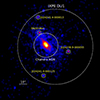 |
Fig. 1. 2.′ × 2.′ central region of NGC 1068, shown in the 0.3–7.0 keV band (Chandra ObsID 29071). The dashed white circle corresponds to the IXPE DU1 source extraction region. A Gaussian smoothing kernel of 3 × 3 pixels has been applied for the sake of visual clarity. |
3. Measurements of NGC 1068’s X-ray polarization
3.1. Imaging X-ray Polarimetry Explorer polarization cubes
We estimated the X-ray polarization properties using the event-based Stokes parameter analysis methods implemented in Kislat et al. (2015). The model-independent analysis was performed using the unweighted method, employing the PCUBE algorithm in ixpeobssim, as is detailed in Baldini et al. (2022). The polarization degree and angle were derived from normalized q and u Stokes parameters, calculated as  and Ψ = 1/2tan−1(u/q) (measured from north to east), with the background polarization subtracted. Consequently, we estimated the time-averaged X-ray polarization properties of the source within the 2–8 keV range as P = 9% ± 5% and Ψ = 113° ± 16°. As is justified in Sect. 2.1, we divided the nominal energy band into two bins and measured P = 14% ± 4% and Ψ = 105° ± 8° (99.7% confidence level) for the energy range 2–5.5 keV. The remaining IXPE band, 5.5–8 keV, only shows an upper limit with P < 20%.
Furthermore, to explore the variability of polarization over time and energy, we segmented the entire observation into subsets based on time and energy, as is described in Kim et al. (2024). Specifically, we divided the q and u data into identical time spans, depending on the selected number of bins, from 2 to 15 bins (2 bins with 1.15 Ms give 575 ks/bin; 15 bins correspond to 77 ks/bin). In all cases, the probability of the hypothesis that the data are constant was greater than 28%, implying no significant evidence of time variability. Energy-resolved analysis was performed in a similar manner. In this case, we divided the 2–8 keV range into 2, 3, 4, 6, 8, and 12 bins (e.g., 2 bins = 2–5 keV, 5–8 keV). The polarization is consistent with being constant with energy, with a probability greater than 24% in all cases. Additional, minor details are shown in the appendix regarding the PCUBE analysis.
3.2. Imaging X-ray Polarimetry Explorer spectropolarimetry
The X-ray spectropolarimetric analysis was carried out with XSPECv12.13.1e (Arnaud 1996). The Galactic absorption along the line of sight amounts to NH, Gal = 2.59 × 1020 cm−2 (HI4PI Collaboration 2016) and was accounted for by using the TBABS model with the interstellar medium abundances from Wilms et al. (2000). We fit the I, Q, and U spectra simultaneously, while including a cross-calibration constant (CONST) between the three different DUs. For what concerns the sole IXPE data, we focused on phenomenological modeling, while a more physical approach is described in the following section. In this case, the X-ray continuum was modeled as a simple power law (POWERLAW) throughout the whole feasible 2–8 keV energy interval.
In order to probe the polarization properties of NGC 1068, we adopted the POLCONST model, which assumes an energy-independent polarization and has two free parameters: P and Ψ. Thus, we first started with a model that can be written as CONST × TBABS × POLCONST × POWERLAW in XSPEC. The spectral fit was clearly unsatisfactory (χ2/d.o.f. = 931/476), since we observed large positive residuals at energies larger than 6 keV, likely owing to the broad iron line complex. We thus added a Gaussian emission line (ZGAUSS) to account for this component, and this led to a significant fit improvement (χ2/d.o.f. = 537/473), implying that Δχ2 = 394 for three degrees of freedom. We fixed the line width to the value of σ = 500 eV returned by the best fit, since the centroid energy cannot be constrained otherwise. Such a broad emission feature was the result of a blend of several emission lines from both neutral and ionized gas (Matt et al. 2004), which we could not individually resolve with IXPE. The emission line was centered at E = 6.58 keV. We found a rather soft X-ray continuum, with the photon index having a value of Γ = 2.35
 .
.
Nonetheless, we still observed some residuals at softer energies, which we tried to account for by including an additional power-law component. This led to a further improvement in the spectral fit (χ2/d.o.f. = 474/472). Thus, our best-fit phenomenological model consists of:

The line centroid shifts toward E = 6.67 ± 0.06 keV and the two power-law photon indices are Γ1 = 0.9 ± 0.4 and Γ2 = 4.3 . The best-fit values of the 2–8 keV polarization degree and angle are P = 12.4% ± 3.6% and Ψ = 100.7° ± 8.3°, respectively.
Finally, we divided the broad energy band into smaller intervals to probe the polarization properties of NGC 1068. The 2–5.5 keV band shows the highest significance in terms of polarization detection. Fig. 2 shows the contour plot of the polarization angle versus the polarization degree in such an interval. At energies higher than 5.5 keV, there is a clear rise of background contribution in addition to the emission lines from the iron K complex that are blended and widened due to the modest IXPE spectral resolution. The results are listed in Table 1 and are generally in good agreement with the values reported from the PCUBE model-independent analysis described in the previous section.
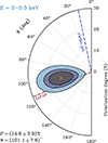 |
Fig. 2. Contour plot of the polarization angle vs. polarization degree accounting for the 68%, 90%, and 99% confidence levels, computed by taking into account the IXPE I, Q, and U spectra in the 2–5.5 keV band (the energy band with the highest significance in terms of polarization detection). The orange cross indicates the best-fit values of P and Ψ, which are also reported in the lower left corner. The dashed blue line describes the direction of the parsec-scale radio jet (Wilson & Ulvestad 1983). The dashed brown line indicates the orientation of the molecular torus derived by García-Burillo et al. (2019) with ALMA (see Sect. 4.1). |
Measured fluxes and polarization.
3.3. Imaging X-ray Polarimetry Explorer+Chandra fitting
Thanks to the Chandra data, we were able to take into account the contribution of the ULXs in the spectral analysis (Bauer et al. 2015). We co-added the Chandra spectra of extranuclear point sources that were significantly detected above 2 keV, and we modeled this combined ULX emission with a power law that has a fixed slope of 1. We obtained a 2–8 keV flux of 2.2 × 10⁻¹³ erg cm−2 s−1 for the ULX power law. The AGN, on the other hand, has a 2–8 keV flux of 4.3 × 10⁻¹² erg cm−2 s−1.
The 2–8 keV continuum is well described by two components: a warm reflector, mostly contributing below 4 keV, and a cold reflector, dominating above 5 keV (see also Matt et al. 2004). In both cases, the reflected continuum is expected to be significantly polarized, while the associated emission lines are expected to be unpolarized. We fit jointly the Chandra and IXPE I, Q, and U Stokes spectra with a phenomenological model consisting of: a power law to describe the warm reflector continuum, a PEXRAV (Magdziarz & Zdziarski 1995) component for the cold reflector continuum, and six Gaussian emission lines2. The photon indices of the warm and cold reflection components were not well constrained by the Chandra + IXPE fit; therefore, we adopted values consistent with those reported by Matt et al. (2004), Marinucci et al. (2016), and Zaino et al. (2020). We fixed the photon index of PEXRAV at 2, and that of the warm reflector at 33. In PEXRAV, the high-energy cut-off was not included, being fixed at the maximum value of 106 keV because the fit is not sensitive to this parameter. The reflection fraction was fixed at −1, which yields the reflection component alone in PEXRAV. To fit the IXPE spectra, we also included the power law describing the ULX emission derived from Chandra, fixing both the photon index and the flux. Finally, we multiplied the different components by the POLCONST model. We assumed that the emission lines and the ULXs were unpolarized4. The XSPEC model is as follows:
![Mathematical equation: $$ \begin{aligned} c\_cal \times tbabs \times&[ polconst ^{(0)} \times ( \textstyle \sum zgauss ^{(i)}&\text{ lines} \\&+ powerlaw )&\text{ ULXs} \\&+ polconst ^{(w)} \times powerlaw&\text{ warm} \text{ refl.}\\&+ polconst ^{(c)} \times pexrav ]&\text{ cold} \text{ refl.} \end{aligned} $$](/articles/aa/full_html/2024/09/aa49760-24/aa49760-24-eq6.gif)
where C_CAL is the cross-calibration constant. We fixed the polarization degree of POLCONST(0) at zero, which must be set in XSPEC to describe an unpolarized component. The polarization angle of POLCONST(0) was also formally set at zero, even though this parameter has no meaning when the polarization degree is zero5. The data and best-fitting model are shown in Figs. 3 and 4.
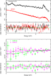 |
Fig. 3. Top panel: Chandra/ACIS and IXPE I spectra with best-fitting model and residuals. Bottom panel: IXPE Q and U Stokes spectra with best-fitting model and residuals. |
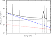 |
Fig. 4. Best-fitting total model (solid black line) for the Chandra+IXPE data. The plot shows the different components: a cold reflection (dotted black line), a warm reflection (dashed blue line), and ULXs (dotted red line). |
We find significant degeneracy among the polarization parameters of the warm and cold reflectors. The contour plot (not shown here) between the polarization degrees of the two components indicates that even at 1-sigma, Pcold is barely above zero and Pwarm has only an upper limit of 28%. To reduce such a degeneracy, we needed to make some assumptions. We thus fixed the polarization parameters of the warm component using the far-UV polarimetric measurements of Antonucci et al. (1994) (see also Sect. 4.3). Those authors have shown that, within the first few arcseconds, electron scattering in the winds is mainly responsible for the far-UV polarization. If electron scattering prevails in the wind, its scattering-induced polarization should be similar from the optical to the X-rays, so we postulated at the first order that the X-ray counterpart could be similar. We thus fixed the polarization degree and angle of the warm reflector at 16% and 97°, respectively. With this assumption, we obtained a good fit with χ2/d.o.f. = 534/527 : the cold reflector has a polarization degree of 20% ± 10% (nonzero at merely two sigma) and a polarization angle of 102° ± 15°. The best-fitting parameters are reported in Table 2.
Best-fitting model.
Finally, we note that the warm reflection component is still expected to be significantly contaminated by unresolved emission lines, in which case the polarization degree could be much lower than our initial assumption. In the extreme hypothesis of null polarization of the warm reflector, we obtain a statistically equivalent fit, and a polarization degree of the cold reflector of 36%±10% with a polarization angle similar to that obtained in the first case.
4. Analysis
4.1. The geometrical distribution of scatterers
The observed X-ray polarization angle can be compared to the position angle (PA) of the parsec-scale radio-jet seen in NGC 1068 to determine whether scattering occurs along the equatorial plane (Ψ − PA ≈ 0°) or in the polar direction (Ψ − PA ≈ 90°). The resolved parsec-scale jet on the 4.9 GHz map of Wilson & Ulvestad (1983) sustains a PA of ∼34°, but the jet does not follow a straight trajectory from the supposed position of the supermassive black hole (S1 component) to the terminal lobes. It is, in fact, deflected to the northeast (see Gallimore et al. 2004). The central, sub-arcsecond jet structure was resolved by VLBA and phased VLA 1.4 GHz observations and the inner PA of the jet (going from component S1 to C) is at about 12° (see Fig. 2 in Gallimore et al. 2004 and also the very precise cartography of the radio emission in NGC 1068 by Mutie et al. 2024). The subtraction gives us 101°–12° = 89°. We thus conclude that the observed X-ray polarization angle of NGC 1068 is perpendicular to the radio structure axis6, implying that the observed X-ray polarization arises from scattering onto material that is preferentially situated well above the equatorial plane.
Two components of the AGN can be responsible for this: the outflows or the torus. Our measurements, reported in Table 1, show that Ψ is similar in the 2–3.5 keV band (where the warm component dominates the X-ray spectrum; see Sect. 3.3) and in the 3.5–6 KeV band, where the cold component takes precedence. Both components thus likely share the polarization PA. While producing perpendicular polarization in a polar wind is trivial (Goosmann & Gaskell 2007), obtaining a similar polarization angle from an equatorial torus implies that scattering must occur inside the funnel and/or on the uppermost (outer) edges of this Compton-thick region. Such a finding is strongly supported by the Atacama Large Millimeter Array (ALMA) observation of an extended patch of linear polarization arising from a spatially resolved elongated nuclear disk of dust of ∼50–60 pc in diameter and oriented along an averaged PA of ∼113° (García-Burillo et al. 2019).
The Chandra map at 0.5″ resolution of the X-ray emission in NGC 1068 presented by Ogle et al. (2003) also supports our conclusion that the X-ray polarization we measured with IXPE mainly originates in the torus. The authors have shown (see their Figs. 3 and 4) that the peak of the 6–8 keV (Fe K) emission is coincident with the nucleus, as would be expected if it were produced in the inner wall of the molecular torus. Surrounding the X-ray peak in the nuclear region, 3–6 keV extended emission is detected, which is attributed to X-rays that have scattered on the outer edge of the torus. The emission from the warm reflector (the ionization cones) is seen in their Chandra 1.3–3 keV map and is dominated by emission from highly ionized Mg, Si, and S. The warm component also appears in their 3–6 keV emission map but it is mostly scattered continuum. Using XSPEC to measure the associated X-ray polarization in those three energy bands (see Table 1) gives only an upper limit to the 6–8 keV emission, resulting from the combination of higher background levels and strong, little-to-no polarized emission from the iron K complex. In the 3.5–6 keV band, where scattering off the torus is prevalent, P rises up to ∼21%. In the softest X-ray band (2–3.5 keV), the observed polarization degree is much lower (∼10%), mostly due to the forest of narrow emission lines that depolarize the signal. Many of those lines are significantly enhanced by photoexcitation, so they might be polarized, albeit at a lower level from the hard continuum.
4.2. Estimating the active galactic nucleus inclination and torus geometry
Even if nothing definitive can be said about the intrinsic polarization degree and angle originating from the torus, we can try to evaluate the geometry of this region thanks to Monte Carlo radiative transfer simulations of optically thick tori. We used the radiative transfer Monte Carlo code STOKES (Goosmann & Gaskell 2007; Marin et al. 2012, 2015; Marin 2018b; Rojas 2018) to simulate a central, isotropical continuum source with a power law index of Γ ∼ 2.04 (Matt et al. 2004, Pounds & Vaughan 2006 and Sect. 3.3). The source emits a 2% parallel polarized primary continuum, since it has been shown in NGC 4151 that the X-ray continuum is polarized in parallel by a few percent (Gianolli et al. 2023). Around the central source, we modeled a uniform-density torus using a circular cross section. The inner wall of the torus was set at a fixed distance of rin = 0.25 pc (Lopez-Rodriguez et al. 2018; Vermot et al. 2021) and the radius, a, of the torus was set by the region’s half-opening angle, Θ, such as a = rin cos Θ/(1-cos Θ). The neutral hydrogen density, NH, was set to 1025 atom cm−2 along the equatorial plane (Matt et al. 2004). The half-opening angle of the torus and the system inclination, i, were free parameters, both measured from the vertical symmetry axis of the system. Type-2 AGNs were thus found for i > Θ. Such models have been examined in detail in Podgorný et al. (2023) and we refer the reader to this publication for in-depth details.
We present in Fig. 5 the results of the simulations for a wide variety of Θ and i angles. The polarization is integrated between 3.5 and 6 keV to avoid as much contamination as possible from the fluorescent and recombination lines (see Fig. 4). Superimposing the estimated neutral reflector X-ray polarization (20% ± 10%) on the models allows us to put strong constraints on the geometrical configuration of the system. Excluding a) all torus half-opening angles smaller than that of the ionized polar winds seen in NGC 1068, which sustain a half-opening angle of 40°, traced by [O III] emission (Macchetto et al. 1994), b) all results for i < Θ, and c) all non-perpendicular polarization angles (an assumption compatible with IXPE data), we find that the range of permitted AGN inclinations is 42°–87° and the range of torus half-opening angles is 40°–57.5° (as is illustrated by the black dots in Fig. 5). Further observation with better statistics could narrow down the parameter space, but if we rely on the range of inclinations, i, estimated from the literature (70°–90°, see Sect. 1), the permitted range of Θ becomes 45°–57.5°, with a much higher probability of being in the range of 50°–55°. Interestingly, this is comparable to the range of Θ found in the case of the Circinus galaxy (45°–55°), the only other type-2 AGN probed by IXPE (Ursini et al. 2023).
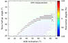 |
Fig. 5. STOKES simulations of a circular torus with various half-opening angles, Θ, seen at several observer inclinations, i. The color-coded polarization degree is integrated from 3.5 to 6.0 keV to avoid any contribution from intense emission lines. A positive polarization degree indicates that the photon electric field vector is parallel to the axis of symmetry of the system. Thus, negative polarization stands for perpendicularly polarized photons. Each colored dot represents a (Θ, i) simulation. If the polarization degree and angle of a dot is consistent with the X-ray polarization of the torus measured by IXPE, the dot is shown in black. |
For the sake of completeness, we also tested the line-dominated warm reflector scenario (P = 0%), which would lead to a neutral reflector polarization of 36%±10% (see Sect. 3.3). In doing so, the torus half-opening angle estimated from Monte Carlo radiative transfer simulations becomes 40°–50°, with a much higher statistical probability of being between 45° and 50°. This is also comparable to the range of Θ found in the case of the Circinus galaxy.
4.3. Comparison with optical data
The broadband polarization of NGC 1068 has been thoroughly examined from the ultraviolet to the infrared band (see Marin 2018a and reference therein for a review). Yet, due to strong starlight dilution by the host, the true (intrinsic) polarization levels of the AGN is difficult to estimate. It is possible to correct the UV-optical polarization for dilution by subtracting the stellar component(s) from the total flux, but this is not an easy process. The addition of the X-ray polarization measurement achieved by IXPE brings another piece to the puzzle, since it is essentially free from diluting sources (apart from the almost negligible ULX signal). A comparison between X-ray and optical data can thus lead to better constraints on the global geometry of the AGN.
To do so, 0.35–1.1 μm linear spectropolarimetry was obtained between December 1 and 6, 2023, with the FOcal Reducer/low dispersion Spectrograph 2 (FORS2) instrument mounted on the Very Large Telescope (VLT), quasi-simultaneously with regard to the IXPE observation. The observation, under program ID 112.26WL.001, will be analyzed and published later on (Marin et al., in prep.), but the reduced optical data confirm that the linear polarization from NGC 1068 has remained stable over the last few decades, especially in the continuum. The polarization degree rises from ∼1.5% in the red up to ∼12% in the blue band. The polarization PA is almost constant with wavelength, slowly rotating from ∼100° in the red to ∼90° in the blue. The rise in P continues in the ultraviolet band up to 16% at a PA of 97° shortward of 2700 Å (Code et al. 1993; Antonucci et al. 1994). The polarization degree then plateaus, as the host starlight contribution becomes negligible, indicating that electron scattering dominates in the winds.
The matching of the polarization angle between the near-infrared, optical, ultraviolet, and X-rays clearly indicates that the polarization results in all cases from scattering by material well above the equatorial plane. But they are not due to the same AGN component. X-ray spectropolarimetry tends to favor light reflection off atoms and molecules from the cold component (the torus), while optical imaging and spectropolarimetry supports electron (or dust) scattering inside the polar outflows (Antonucci & Miller 1985; Antonucci et al. 1994). In the spectral region where emission from the ionized winds dominates the X-ray signal (2–3.5 keV; see Fig. 4), we measured P = 9.8% ± 4.9% at 104.2° ± 14.9°. Although diluted by the emission lines, the polarized X-ray continuum probably comes from the optically thin region that scatters the optical and ultraviolet photons (Antonucci & Miller 1985).
As things currently stand and with the statistics offered by our observation, we note that the optical-ultraviolet and X-ray measurements are different in P (but not in Ψ), so we caution against using ultraviolet polarization measurements of Seyfert-2 galaxies as a basic proxy to predict the polarization level of a source in the X-rays.
5. Conclusions
We have measured the 2–8 keV polarization of the archetypal Seyfert-2 AGN NGC 1068 with IXPE. We find a linear polarization degree of 12.4% ± 3.6% at 100.7° ± 8.3° (68% confidence level). The polarization is perpendicular to the PA of the parsec-scale radio structure, similar to what is observed for all Seyfert-2s in the optical band. A combined Chandra and IXPE analysis indicates a significant degeneracy among the polarization parameters of the warm and cold reflectors but, from multiwavelength constraints, we estimate that the cold reflector has a polarization degree of 20% ± 10% and polarization angle of 102° ± 15°. Taking the result at face value, we used numerical simulations to derive a probable torus half-opening angle of 50–55° (from the vertical axis of the system). This morphological constraint is quite similar to the torus half-opening angle derived for the Circinus galaxy thanks to X-ray polarimetry, the only other type-2 AGN probed by IXPE so far. In producing this result, X-ray polarimetry has shown its powerful and unique capability to constrain the geometrical arrangement of matter around supermassive black holes.
The adopted script is available on https://github.com/aledimarco/IXPE-background
We used PEXRAV plus emission lines instead of models that self-consistently include both the continuum and the lines because the polarization of the reflected continuum and of the emission lines was expected to be different (see also Ursini et al. (2023)).
The soft spectrum is steeper than the primary continuum because it is dominated by recombination and resonant lines (Guainazzi & Bianchi 2007), which are mostly unresolved in our case. However, we checked that we obtained consistent polarimetric results if we fixed the photon index of the warm reflector at 2, or if we left it free to vary.
The ULXs are likely polarized, with P depending on their true nature, orientation, and geometry (Veledina et al. 2023). However, the ULXs around NGC 1068 contribute so weakly to the total flux that assuming no polarization is a reasonable hypothesis.
If we left POLCONST(0) free to vary, we only obtained loose constraints, with a 1-sigma upper limit to the polarization degree of 30%. We also tried to assess the contribution to the observed polarization by the emission lines and ULXs separately, via the multiplication of POLCONST with the ZGAUSS and POWERLAW components. In this case, we obtained a 1-sigma upper limit of 60% to the polarization of the ULXs component and of 40% to the polarization of the lines.
We note that the higher-resolution VLBA images in Gallimore et al. (2004) show a torus structure for S1 (see their Figs. 3c and 4c), with a PA of 104.5°–108.1°, which is again a very good match with the X-ray polarization angle that we measured.
Acknowledgments
The Imaging X-ray Polarimetry Explorer (IXPE) is a joint US and Italian mission. The US contribution is supported by the National Aeronautics and Space Administration (NASA) and led and managed by its Marshall Space Flight Center (MSFC), with industry partner Ball Aerospace (contract NNM15AA18C). The Italian contribution is supported by the Italian Space Agency (Agenzia Spaziale Italiana, ASI) through contract ASI-OHBI-2022-13-I.0, agreements ASI-INAF-2022-19-HH.0 and ASI-INFN-2017.13-H0, and its Space Science Data Center (SSDC) with agreements ASI-INAF-2022-14-HH.0 and ASI-INFN 2021-43-HH.0, and by the Istituto Nazionale di Astrofisica (INAF) and the Istituto Nazionale di Fisica Nucleare (INFN) in Italy. This research used data products provided by the IXPE Team (MSFC, SSDC, INAF, and INFN) and distributed with additional software tools by the High-Energy Astrophysics Science Archive Research Center (HEASARC), at NASA Goddard Space Flight Center (GSFC). F.M. thanks Robert Antonnucci, Makoto Kishimoto, Patrick Ogle and Ari Laor for their valuable comments on the manuscript. A.D.M., E.Co., R.F., S.F., F.L.M., F. Mu. P.So. are partially supported by MAECI with grant CN24GR08 “GRBAXP: Guangxi-Rome Bilateral Agreement for X-ray Polarimetry in Astrophysics”. F.T. and M.L. acknowledge funding from the European Union – Next Generation EU, PRIN/MUR 2022 (2022K9N5B4). M.D., J.P., and V.K. thank GACR project 21-06825X for the support and institutional support from RVO:67985815. I.L. was supported by the NASA Postdoctoral Program at the Marshall Space Flight Center, administered by Oak Ridge Associated Universities under contract with NASA. The work of RTa and RTu is partially supported by grant PRIN-2022LWPEXW of the Italian MUR. The French contribution (F.M., T.B., V.E.G., P.-O.P.) is partly supported by the French Space Agency (Centre National d’Etude Spatiale, CNES) and by the High Energy National Programme (PNHE) of the Centre National de la Recherche Scientifique (CNRS). The authors thank the anonymous referee for her/his helpful comments that improved the quality of the manuscript.
References
- Antonucci, R. 1993, ARA&A, 31, 473 [Google Scholar]
- Antonucci, R. R. J., & Miller, J. S. 1985, ApJ, 297, 621 [NASA ADS] [CrossRef] [Google Scholar]
- Antonucci, R., Hurt, T., & Miller, J. 1994, ApJ, 430, 210 [NASA ADS] [CrossRef] [Google Scholar]
- Arnaud, K. A. 1996, ASP Conf. Ser., 101, 17 [Google Scholar]
- Baldini, L., Bucciantini, N., Lalla, N. D., et al. 2022, Astrophysics Source Code Library [record ascl:2210.020] [Google Scholar]
- Bauer, F. E., Arévalo, P., Walton, D. J., et al. 2015, ApJ, 812, 116 [Google Scholar]
- Bostroem, K. A., Valenti, S., Sand, D. J., et al. 2020, ApJ, 895, 31B [NASA ADS] [CrossRef] [Google Scholar]
- Cash, W. 1979, ApJ, 228, 939 [Google Scholar]
- Code, A. D., Meade, M. R., Anderson, C. M., et al. 1993, ApJ, 403, L63 [CrossRef] [Google Scholar]
- Das, V., Crenshaw, D. M., Kraemer, S. B., & Deo, R. P. 2006, AJ, 132, 620 [Google Scholar]
- Di Marco, A., Costa, E., Muleri, F., et al. 2022, AJ, 163, 170 [NASA ADS] [CrossRef] [Google Scholar]
- Di Marco, A., Soffitta, P., Costa, E., et al. 2023, AJ, 165, 143 [CrossRef] [Google Scholar]
- Dopita, M. A. 1997, PASA, 14, 230 [CrossRef] [Google Scholar]
- Fischer, T. C., Crenshaw, D. M., Kraemer, S. B., & Schmitt, H. R. 2013, ApJS, 209, 1 [Google Scholar]
- Fruscione, A., McDowell, J., Allen, G., et al. 2006, SPIE Conf. Ser., 6270 [Google Scholar]
- Gámez, Rosas V., Isbell, J. W., Jaffe, W., et al. 2022, Nature, 602, 403 [CrossRef] [Google Scholar]
- Gallimore, J. F., Henkel, C., Baum, S. A., et al. 2001, ApJ, 556, 694 [Google Scholar]
- Gallimore, J. F., Baum, S. A., & O’Dea, C. P. 2004, ApJ, 613, 794 [Google Scholar]
- García-Burillo, S., Combes, F., Ramos, Almeida C., et al. 2019, A&A, 632, A61 [NASA ADS] [CrossRef] [EDP Sciences] [Google Scholar]
- Garmire, G. P., Bautz, M. W., Ford, P. G., Nousek, J. A., & Ricker, G. R. 2003, SPIE Conf. Ser., 4851, 28 [NASA ADS] [Google Scholar]
- Gianolli, V. E., Kim, D. E., Bianchi, S., et al. 2023, MNRAS, 523, 4468 [NASA ADS] [CrossRef] [Google Scholar]
- Goosmann, R. W., & Gaskell, C. M. 2007, A&A, 465, 129 [NASA ADS] [CrossRef] [EDP Sciences] [Google Scholar]
- Goosmann, R. W., & Matt, G. 2011, MNRAS, 415, 3119 [NASA ADS] [CrossRef] [Google Scholar]
- Greenhill, L. J., Gwinn, C. R., Antonucci, R., & Barvainis, R. 1996, ApJ, 472, L21 [Google Scholar]
- Guainazzi, M., & Bianchi, S. 2007, MNRAS, 374, 1290 [Google Scholar]
- Hönig, S. F., Beckert, T., Ohnaka, K., & Weigelt, G. 2007, ASP Con. Ser., 373, 487 [Google Scholar]
- Hönig, S. F., Prieto, M. A., & Beckert, T. 2008, A&A, 485, 33 [NASA ADS] [CrossRef] [EDP Sciences] [Google Scholar]
- HI4PI Collaboration (Ben Bekhti, N., et al.) 2016, A&A, 594, A116 [NASA ADS] [CrossRef] [EDP Sciences] [Google Scholar]
- Ingram, A., Ewing, M., Marinucci, A., et al. 2023, MNRAS, 525, 5437 [CrossRef] [Google Scholar]
- Kim, D. E., Di Gesu, L., Liodakis, I., et al. 2024, A&A, 681, A12 [NASA ADS] [CrossRef] [EDP Sciences] [Google Scholar]
- Kishimoto, M. 1999, ApJ, 518, 676 [NASA ADS] [CrossRef] [Google Scholar]
- Kislat, F., Clark, B., Beilicke, M., & Krawczynski, H. 2015, APh, 68, 45 [NASA ADS] [Google Scholar]
- Lopez-Rodriguez, E., Fuller, L., Alonso-Herrero, A., et al. 2018, ApJ, 859, 99 [Google Scholar]
- Macchetto, F., Capetti, A., Sparks, W. B., Axon, D. J., & Boksenberg, A. 1994, ApJ, 435, L15 [Google Scholar]
- Maeda, K., Chandra, P., Moriya, T. J., et al. 2023, ApJ, 942, 17 [NASA ADS] [CrossRef] [Google Scholar]
- Magdziarz, P., & Zdziarski, A. A. 1995, MNRAS, 273, 837 [Google Scholar]
- Marin, F., Goosmann, R. W., Gaskell, C. M., Porquet, D., & Dovčiak, M. 2012, A&A, 548, A121 [NASA ADS] [CrossRef] [EDP Sciences] [Google Scholar]
- Marin, F., Dovčiak, M., Muleri, F., Kislat, F. F., & Krawczynski, H. S. 2018, MNRAS, 473, 1286 [NASA ADS] [CrossRef] [Google Scholar]
- Marin, F., Goosmann, R. W., & Gaskell, C. M. 2015, A&A, 577, A66 [NASA ADS] [CrossRef] [EDP Sciences] [Google Scholar]
- Marin, F., Goosmann, R. W., & Petrucci, P.-O. 2016, A&A, 591, A23 [NASA ADS] [CrossRef] [EDP Sciences] [Google Scholar]
- Marin, F. 2018a, MNRAS, 479, 3142 [NASA ADS] [CrossRef] [Google Scholar]
- Marin, F. 2018b, A&A, 615, A171 [NASA ADS] [CrossRef] [EDP Sciences] [Google Scholar]
- Marinucci, A., Bianchi, S., Matt, G., et al. 2016, MNRAS, 456, L94 [Google Scholar]
- Marinucci, A., Muleri, F., Dovciak, M., et al. 2022, MNRAS, 516, 5907 [NASA ADS] [CrossRef] [Google Scholar]
- Matt, G., Bianchi, S., Guainazzi, M., & Molendi, S. 2004, A&A, 414, 155 [NASA ADS] [CrossRef] [EDP Sciences] [Google Scholar]
- Miyauchi, R., & Kishimoto, M. 2020, ApJ, 904, 149 [NASA ADS] [CrossRef] [Google Scholar]
- Mutie, I. M., Williams-Baldwin, D., Beswick, R. J., et al. 2024, MNRAS, 527, 11756 [Google Scholar]
- Ogle, P. M., Brookings, T., Canizares, C. R., Lee, J. C., & Marshall, H. L. 2003, A&A, 402, 849 [NASA ADS] [CrossRef] [EDP Sciences] [Google Scholar]
- Packham, C., Young, S., Hough, J. H., Axon, D. J., & Bailey, J. A. 1997, MNRAS, 288, 375 [CrossRef] [Google Scholar]
- Pal, I., Stalin, C. S., Chatterjee, R., & Agrawal, V. K. 2023, JApA, 44, 87 [NASA ADS] [Google Scholar]
- Piconcelli, E., Jimenez-Bailón, E., Guainazzi, M., et al. 2004, MNRAS, 351, 161 [Google Scholar]
- Podgorný, J., Marin, F., & Dovčiak, M. 2023, MNRAS, 526, 4929 [CrossRef] [Google Scholar]
- Podgorný, J., Marin, F., & Dovčiak, M. 2024, MNRAS, 527, 1114 [Google Scholar]
- Pounds, K., & Vaughan, S. 2006, MNRAS, 368, 707 [Google Scholar]
- Romeo, A. B., & Fathi, K. 2016, MNRAS, 460, 2360 [NASA ADS] [CrossRef] [Google Scholar]
- Rojas, Lobos P. A., & Goosmann R. W., Marin F., Savić D., 2018, A&A, 611, A39 [NASA ADS] [CrossRef] [EDP Sciences] [Google Scholar]
- Sandage, A. 1973, ApJ, 183, 711 [NASA ADS] [CrossRef] [Google Scholar]
- Smith, D. A., & Wilson, A. S. 2003, ApJ, 591, 138 [NASA ADS] [CrossRef] [Google Scholar]
- Tagliacozzo, D., Marinucci, A., Ursini, F., et al. 2023, MNRAS, 525, 4735 [CrossRef] [Google Scholar]
- Tinbergen, J. 2005, Astronomical Polarimetry (Cambridge, UK: Cambridge University Press), 176 [Google Scholar]
- Urry, C. M., & Padovani, P. 1995, PASP, 107, 803 [NASA ADS] [CrossRef] [Google Scholar]
- Ursini, F., Marinucci, A., Matt, G., et al. 2023, MNRAS, 519, 50 [Google Scholar]
- Veledina, A., Muleri, F., Poutanen, J., et al. 2023, ArXiv e-prints [arXiv:2303.01174] [Google Scholar]
- Vermot, P., Clénet, Y., Gratadour, D., et al. 2021, A&A, 652, A65 [NASA ADS] [CrossRef] [EDP Sciences] [Google Scholar]
- Weisskopf, M. C., Elsner, R. F., & O’Dell, S. L. 2010, SPIE Con. Ser., 7732, 77320E [NASA ADS] [Google Scholar]
- Weisskopf, M. C., Soffitta, P., Baldini, L., et al. 2022, JATIS, 8, 026002 [NASA ADS] [Google Scholar]
- Wilms, J., Allen, A., & McCray, R. 2000, ApJ, 542, 914 [Google Scholar]
- Wilson, A. S., & Ulvestad, J. S. 1983, ApJ, 275, 8 [Google Scholar]
- Zaino, A., Bianchi, S., Marinucci, A., et al. 2020, MNRAS, 492, 3872 [Google Scholar]
Appendix A: Summary of PCUBE analysis
In order not to confuse the reader with both the PCUBE and XSPEC results in the main body of the article, we summarize here our findings using a PCUBE analysis. We computed the significance of detection for a variety of energy bins, calculated in the same way as that presented in Sect. 3.1, considering two degrees of freedom and following the official IXPE statistical guide7. We also detail the variability observed in both time and energy domains for three separate bins. Our results can be found in Tab. A.1.
Results from our PCUBE analysis.
As is shown in the table, the most solid detections are found in the 2 – 5.5 and 2 – 6 keV bands, before the onset of fluorescent emission from the iron K complex and its associated dilution. The values measured in those energy bands are above the minimum detectable polarization; that is, the degree of polarization corresponding to the amplitude of modulation that has only a 1% probability of being detected by chance (Weisskopf et al. 2010).
Regarding the variability tests mentioned in Sect. 3.1, we show in Fig. A.1 the null hypothesis tests of polarization variability over time (top) and energy (bottom). The lowest probability in the time binning case is 27.63%, and in the energy binning case is 23.80%. In all cases, the polarization appears to be consistent with being constant in time and energy.
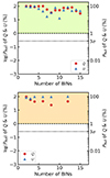 |
Fig. A.1. Null hypothesis probability of the chi-square test for the constant model on the normalized Q (red) and U (blue) Stokes parameters for different time (top panel) and energy (bottom panel) binning cases. The left and right vertical axes in each panel show the percentage of the probability values on a logarithmic and linear scale, respectively. The shaded green and orange areas indicate the 1% threshold level. The dashed and dotted black lines in the middle of each panel represent the 1% and 3σ (99.73%) probability levels, respectively. |
All Tables
All Figures
|
Fig. 1. 2.′ × 2.′ central region of NGC 1068, shown in the 0.3–7.0 keV band (Chandra ObsID 29071). The dashed white circle corresponds to the IXPE DU1 source extraction region. A Gaussian smoothing kernel of 3 × 3 pixels has been applied for the sake of visual clarity. |
| In the text | |
|
Fig. 2. Contour plot of the polarization angle vs. polarization degree accounting for the 68%, 90%, and 99% confidence levels, computed by taking into account the IXPE I, Q, and U spectra in the 2–5.5 keV band (the energy band with the highest significance in terms of polarization detection). The orange cross indicates the best-fit values of P and Ψ, which are also reported in the lower left corner. The dashed blue line describes the direction of the parsec-scale radio jet (Wilson & Ulvestad 1983). The dashed brown line indicates the orientation of the molecular torus derived by García-Burillo et al. (2019) with ALMA (see Sect. 4.1). |
| In the text | |
|
Fig. 3. Top panel: Chandra/ACIS and IXPE I spectra with best-fitting model and residuals. Bottom panel: IXPE Q and U Stokes spectra with best-fitting model and residuals. |
| In the text | |
|
Fig. 4. Best-fitting total model (solid black line) for the Chandra+IXPE data. The plot shows the different components: a cold reflection (dotted black line), a warm reflection (dashed blue line), and ULXs (dotted red line). |
| In the text | |
|
Fig. 5. STOKES simulations of a circular torus with various half-opening angles, Θ, seen at several observer inclinations, i. The color-coded polarization degree is integrated from 3.5 to 6.0 keV to avoid any contribution from intense emission lines. A positive polarization degree indicates that the photon electric field vector is parallel to the axis of symmetry of the system. Thus, negative polarization stands for perpendicularly polarized photons. Each colored dot represents a (Θ, i) simulation. If the polarization degree and angle of a dot is consistent with the X-ray polarization of the torus measured by IXPE, the dot is shown in black. |
| In the text | |
|
Fig. A.1. Null hypothesis probability of the chi-square test for the constant model on the normalized Q (red) and U (blue) Stokes parameters for different time (top panel) and energy (bottom panel) binning cases. The left and right vertical axes in each panel show the percentage of the probability values on a logarithmic and linear scale, respectively. The shaded green and orange areas indicate the 1% threshold level. The dashed and dotted black lines in the middle of each panel represent the 1% and 3σ (99.73%) probability levels, respectively. |
| In the text | |
Current usage metrics show cumulative count of Article Views (full-text article views including HTML views, PDF and ePub downloads, according to the available data) and Abstracts Views on Vision4Press platform.
Data correspond to usage on the plateform after 2015. The current usage metrics is available 48-96 hours after online publication and is updated daily on week days.
Initial download of the metrics may take a while.