| Issue |
A&A
Volume 689, September 2024
|
|
|---|---|---|
| Article Number | A333 | |
| Number of page(s) | 15 | |
| Section | Extragalactic astronomy | |
| DOI | https://doi.org/10.1051/0004-6361/202449388 | |
| Published online | 23 September 2024 | |
Disentangling the X-ray variability in the Lyman continuum emitter Haro 11
1
Eureka Scientific, 2452 Delmer Street, Suite 100, Oakland, CA 94602-3017, USA
2
Instituto Nacional de Astrofísica, Óptica y Electrónica (INAOE), AP 51, 72000 Puebla, Mexico
3
Inter-University Centre for Astronomy and Astrophysics (IUCAA), Pune University Campus, Pune 411007, India
4
Department of Astronomy, Oskar Klein Centre, Stockholm University, AlbaNova, SE-106 91 Stockholm, Sweden
Received:
29
January
2024
Accepted:
19
June
2024
Context. Lyman break analogs in the local Universe serve as counterparts to Lyman break galaxies (LBGs) at high redshifts, which are widely regarded as major contributors to cosmic reionization in the early stages of the Universe.
Aims. We studied XMM-Newton and Chandra observations of the nearby LBG analog Haro 11, which contains two X-ray-bright sources, X1 and X2. Both sources exhibit Lyman continuum (LyC) leakage, particularly X2.
Methods. We analyzed the X-ray variability using principal component analysis (PCA) and performed spectral modeling of the X1 and X2 observations made with the Chandra ACIS-S instrument.
Results. The PCA component, which contributes to the X-ray variability, is apparently associated with variable emission features, likely from ionized superwinds. Our spectral analysis of the Chandra data indicates that the fainter X-ray source, X2 (X-ray luminosity LX ∼ 4 × 1040 erg s−1), the one with higher LyC leakage, has a much lower absorbing column (NH ∼ 1.2 × 1021 cm−2) than the heavily absorbed luminous source X1 (LX ∼ 9 × 1040 erg s−1 and NH ∼ 11.5 × 1021 cm−2).
Conclusions. We conclude that X2 is likely less covered by absorbing material, which may be a result of powerful superwinds clearing galactic channels and facilitating the escape of LyC radiation. Much deeper X-ray observations are required to validate the presence of potential superwinds and determine their implications for the LyC escape.
Key words: galaxies: dwarf / galaxies: starburst / X-rays: galaxies
© The Authors 2024
 Open Access article, published by EDP Sciences, under the terms of the Creative Commons Attribution License (https://creativecommons.org/licenses/by/4.0), which permits unrestricted use, distribution, and reproduction in any medium, provided the original work is properly cited.
This article is published in open access under the Subscribe to Open model. Subscribe to A&A to support open access publication.
1. Introduction
X-ray observations of Lyman continuum (LyC) emitters in the early Universe face significant challenges due to their considerable distance. Our understanding of their X-ray characteristics is inferred from stacking analyses (Nandra et al. 2002; Lehmer et al. 2005; Laird et al. 2006; Zinn et al. 2012; Basu-Zych et al. 2013) and optimized averaging analysis (Cowie et al. 2012). The high redshifts of distant galaxies result in the rest-frame X-rays shifting into the energy range below a few keV. However, the extinction caused by the intergalactic medium, poor spatial resolutions, and low signal-to-noise ratios of distant galaxies preclude us from getting a complete picture of the X-ray properties of high-z LyC emitters, which could contribute to the majority of the early Universe’s ionizing budget (Barkana & Loeb 2001; Robertson et al. 2010; Dayal & Ferrara 2018). Because of this complication, it is difficult to study the X-ray features of high-z starburst galaxies. However, a detailed X-ray analysis of their nearby analogs helps us better understand the X-ray properties of LyC emitters in the faraway Universe.
Haro 11 (ESO 350-IG 038) is the closest LyC leaking dwarf galaxy (Bergvall et al. 2006; Leitet et al. 2011; Rivera-Thorsen et al. 2017; Östlin et al. 2021; Komarova et al. 2024) in the local Universe (z = 0.0206 and D = 82 Mpc; Micheva et al. 2010) that shares many characteristics with Lyman break galaxies (LBGs) in the early Universe (Grimes et al. 2007). It is also classified as a Lyα-emitting source, and its young star-cluster population is similar to those of high-z Lyα emitters (Hayes et al. 2007). The Lyα leakage in this galaxy has been confirmed by means of UV imaging (Östlin et al. 2009, 2021) and UV spectroscopy (Rivera-Thorsen et al. 2017). This compact blue galaxy has a high star formation rate of ∼20–28.6 M⊙ yr−1 (Grimes et al. 2007; Madden et al. 2013) and a relatively low metallicity of 12 + [O/H] = 7.9 (Östlin et al. 2015), similar to LBGs at high redshifts. It has been extensively studied in the IR, optical, UV, and X-ray (e.g., Bergvall et al. 2000; Hayes et al. 2007; Östlin et al. 2009; Adamo et al. 2010; Cormier et al. 2012; Prestwich et al. 2015; Gross et al. 2021). It contains three optically bright predominant knots, labeled A, B, and C in the Hubble Space Telescope (HST) observations (see Fig. 1, top). Each of these knots comprises several super star clusters (SSCs), with ages ranging from 1 to 40 Myr, and has an average star formation rate of around 22 M⊙ yr−1 (Adamo et al. 2010). The LyC escape fraction was deduced to be around 30% in Knot C, but much lower in Knot B (Östlin et al. 2021). More recently, the LyC escape fractions within 903–912 Å were recently estimated to be 3.4 ± 2.9% in Knot B and 5.1 ± 4.3% in Knot C (Komarova et al. 2024). Haro 11, which is analogous with high-z starburst galaxies (Sirressi et al. 2022), allows us to study the X-ray characteristics of an LBG analog with LyC leakage that is similar to LBGs in the early Universe.
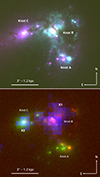 |
Fig. 1. Multiband composite images of Haro 11. Top panel: HST WFC3/UVIS observations using the F555W (blue), F665N (green), and F814W (red) filters (Prop. ID 15649, PI. Chandar). Bottom panel: Multiband imaging in Hα emission (HST F665N, Prop. ID 15649; red), Lyα emission (HST ACS/SBC F122M, Prop. ID 9470; green), and the X-ray 3–5 keV band (Chandra ACIS-S, Obs. ID 8175; blue). The HST data are available via MAST at doi:https://doi.org/10.17909/rn22-jy61. |
Knot B in Haro 11 is coincident with the X-ray source X1 (CXOU J003652.4-333316; see Fig. 1), which contains extremely hard (3–5 keV) X-rays (LX ∼ 1041 erg s−1; Prestwich et al. 2015; Gross et al. 2021). It is likely that the X-rays in X1 originate from an active galactic nucleus (AGN) or an extreme black hole binary (BHB; Prestwich et al. 2015). Knot B is surrounded by an extended superbubble visible in Hα emission (Menacho et al. 2019), which is likely powered by the star cluster wind. X-ray observations also show that Knot C is coincident with the X-ray source X2 (CXOU J003652.7-333316; Fig. 1, bottom), which could be associated with an ultra-luminous X-ray (ULX) source (LX ∼ 5–6 × 1040 erg s−1; Gross et al. 2021). More recently, Komarova et al. (2024) found that both X1 and X2 host ULXs. The X2 source could be capable of powering a strong superwind that could form channels in the surrounding interstellar medium (ISM) while creating a fragmented kiloparsec-scale superbubble (Menacho et al. 2019). In addition, the ISM around X2 was found to be less dense than around X1 (Menacho et al. 2021) and to have a larger Lyα escape fraction (Rivera-Thorsen et al. 2017; Östlin et al. 2021) than the entire region (∼3%; Hayes et al. 2007). Moreover, the ISM around X2 was also found to be hotter (∼16 600 K) and with a lower metallicity (0.12 Z⊙) than that around X1 (∼12 500 K, 0.35 Z⊙; James et al. 2013). Additionally, while X1 was seen to have a greater metal enrichment in integral field spectroscopic observations with the Multi Unit Spectroscopic Explorer (MUSE) on the Very Large Telescope (VLT), X2 was found to have higher temperature discrepancies, which could be partially due to shock ionization (Menacho et al. 2021).
Multiband imaging analysis of Haro 11 by Adamo et al. (2010) revealed over 200 young and massive SSCs (masses in the range 104–107 M⊙) that mostly emerged during the starburst that ignited about 40 Myr ago. In addition, supernova explosions could have begun in about half of the SSCs around 3.5 Myr ago. The frequent occurrence of supernova explosions, as found by Sirressi et al. (2022), can lead to hot gas winds around the knots, which illuminate in the diffuse X-ray emission. Previously, Gross et al. (2021) classified the diffuse emission in the vicinity of Knots B and C as the “AGN/composite” region of the Baldwin–Phillips–Telervich (BPT) diagram. However, Sirressi et al. (2022) find that their emission lines are situated around the error margins of the line dividing starbursts from AGNs in the BPT diagram. As mentioned by Menacho et al. (2021), the substantial energy deposition from stellar feedback and supernovae during the recent starburst can generate the observed outflows, resulting in the observed diffuse soft X-ray emission. Menacho et al. (2021) also conclude that Knot C (X2), home to about 80 percent of the supernovae that occurred in Haro 11 in the last 10 Myrs, is the dominant source of energy released in supernova explosions in the system.
The X-ray variability in Chandra observations of Haro 11 has recently been investigated by Gross et al. (2021), who argue for flaring and fading similar to what is seen in the young starburst region of M82 and possible links to the Lyα and LyC emission. As M82 (D = 3.6 Mpc) is much closer than Haro 11, it provides much better X-ray details. In particular, several H-like and He-like emission lines caused by X-ray outflows have been identified in X-ray observations of M82 (Ranalli et al. 2008; Liu et al. 2011; Lopez et al. 2020). Specifically, the link between X-ray variability and outflows has been found in some ULXs (Pinto et al. 2017; Kosec et al. 2018) and quasars (Parker et al. 2017, 2018). Moreover, Heil & Vaughan (2010) found time delays between the hard and soft energy bands in ULXs, which may be caused by different locations of stratification layers in the X-ray outflow leading to X-ray variability. To better evaluate the nature of the X-ray variability in Haro 11 and the possible evidence for outflows, we used principal component analysis (PCA), which serves as a statistical instrument for investigating the variability possibly caused by distinctive ionization zones of potential X-ray outflows as suggested by Parker et al. (2018). In this study we conducted PCA, along with spectral analysis, to disentangle the spectral variability of the X-ray sources. In Sect. 2 we describe the data reduction. In Sect. 3 we analyze the light curves using the hardness ratios and statistical methods, and perform PCA on the X-ray variability. Additionally, we use absorbed spectral models to reproduce the continua and simulate emission lines in the spectra. Our findings are discussed in Sect. 4, which is followed by a conclusion in Sect. 5.
2. Data
Haro 11 was observed with the XMM-Newton telescope (Jansen et al. 2001) in 2004 and 2005, followed by the Chandra X-ray Observatory (CXO; Weisskopf et al. 2000, 2002) in 2006 and 2015–17. Table 1 presents the observation log, including the instruments, exposure times, observing and operating modes. We used observations from the European Photo Imaging Camera-pn (EPIC-pn; Strüder et al. 2001) and the Metal Oxide Semiconductor (MOS) camera (Turner et al. 2001) on XMM. The energy coverage includes the energies from 0.15 to 12 keV with a point spread function (PSF) resolution of 6″ (full width at half maximum). We also retrieved observations made by the Advanced CCD Imaging Spectrometer S-array (ACIS-S; Garmire et al. 2003) from the Chandra Data Archive (CDA). The Chandra dataset is available via the CDA at doi:https://doi.org/10.25574/cdc.219. The ACIS-S, characterized by minimal instrumental background, is capable of covering an energy range from 0.2 to 10 keV with a spatial resolution of 0.492″ (CCD pixel size).
Observation log of Haro 11.
We obtained the original data files (ODFs) of Haro 11 from the XMM-Newton Science Archive. The data were reprocessed with the XMM Science Analysis Software (SAS v 20.0.0; Gabriel et al. 2004) and the current calibration files (XMM-CCF-REL-391) available since 2022 October 25, and adhered to the guidelines outlined in the XMM ABC Guide1. The calibration index files (CIF) and ODFs were produced with the SAS tasks cifbuild and odfingest, correspondingly. The pn and MOS2 event files were generated via the SAS tasks epchain and emchain, respectively. To clean flaring particle background, we excluded the largely contaminated events at the beginning (∼3.5 hours) of each observation, as well as a few of the subsequent events with count rates higher than, respectively, 0.4 and 0.35 c s−1 identified in the single-pixel (PATTERN = 0) 100 s-binned light curves of the 10–12 keV band for pn and > 10 keV for MOS2. Furthermore, the final cleaned events were subjected to filtration using the SAS tool evselect in order to exclusively retain patterned events (pn: PATTERN ≤ 4 and MOS2: PATTERN ≤ 12) and the appropriate PI channels (pn: 200 < PI < 15 000 and MOS2: 200 < PI < 12 000), while excluding any defective pixels (FLAG = 0). The SAS tool edetect_chain was used to locate X-ray sources in the data with the aid of the attitude file made with atthkgen and the band image created by evselect. The SAS task especget was used to extract the source spectra, as well as the related background spectra, redistribution matrix files (RMF), and auxiliary response files (ARF). The source spectrum of each observation was obtained by extracting data from a circular aperture with a radius of 36″ centered on the brightest source. In contrast, the background spectrum was collected from a circular region of the same size and located on the same chip, but positioned distant from the PSF source wings and devoid of any sources. Haro 11 was located near to the edge of the detector only in the EPIC-pn data in 2004 and the MOS2 in 2005.
The Chandra Interactive Analysis of Observations package (CIAO v 4.15; Fruscione et al. 2006) was used to acquire the ACIS-S observations of Haro 11 from the CDA, and reprocess them using the CALDB files (v 4.10.2). The tool specextract provided by CIAO for imaging-mode and zeroth-order grating data was employed to create pulse height amplitude (PHA) files with dmextract, as well as their redistribution and response files using mkrmf and mkarf. We customized this tool (correctpsf = yes, weight = no) in order to apply an energy-dependent point-like PSF correction to the final ARF via the CIAO task arfcorr. The spectra of the X-ray sources X1 and X2 labeled in Fig. 1 were extracted from circular regions with radii of, respectively, 1.6″ and 1.1″ located on their emission peaks. The background was selected from a source-free circular region with a radius of 12″.
3. Analysis
3.1. Timing analysis
To better evaluate the possible variability of the X-ray sources in this galaxy, we generated light curves over several energy ranges. We selected the soft (S: 0.4–1.1 keV), the medium (M: 1.1–2.6 keV), and the hard (H: 2.6–10 keV) bands, with the exception of the Chandra data, where the hard band was limited to 2.6–8 keV. The data series was discretized into time intervals of 1 hour to ensure enough counts (≳5) per bin, in addition to the clear capture of hourly variations. For the XMM data, the SAS procedure evselect was used to extract light curves of the sources and backgrounds for the specified energy ranges. To compensate for the difference in the effective areas, the MOS2 light curves were scaled up using the ratio of the integrated effective areas of pn to MOS2 for each energy band2. Time-binned light curves of the sources resolved by the Chandra telescope were produced with the CIAO tool dmextract for X1 and X2 using the extraction apertures defined in Sect. 2. To compensate for the decrease in the ACIS-S effectiveness over time, the light curves of the observations following the first one were scaled up according to the integration of the effective areas from the ARF over the specified energy range. The soft excess of either an AGN or BHB, which may be present in X1, is usually characterized by a blackbody spectrum likely from the accretion disk. Moreover, powerful ionized superwinds can produce multicomponent warm absorbers, which might be present in the medium band. The coronal, hot plasma within the innermost accretion flow around a black hole can also generate the continuum in the hard excess, commonly described by power law.
To observe any transient changes in the spectral hardness, we also computed the hardness ratios HR1 and HR2 using the light curves of the soft (S), medium (M), and hard (H) bands (H) as follows:

The similar approach was first introduced by Prestwich et al. (2003) for classifying X-ray sources. Hardness ratio analyses appear to be useful to constrain the actual nature of transient phenomena in various objects, such as low-mass X-ray binaries (e.g., Finoguenov & Jones 2002), symbiotic binaries (Danehkar et al. 2021a), and characterize X-ray sources in starbursts (Soria & Wu 2003) and quasi-stellar objects (Danehkar et al. 2018; Boissay-Malaquin et al. 2019).
Figure 2 shows the light curves, including counts summed over S + M and M + H bands (upper panels), and the hardness rations HR1 and HR2 (lower panels). The background-subtracted counts and the associated 1-σ uncertainties were determined from the source and background light curves using the Gaussian quadrature method of the Bayesian Estimator for Hardness Ratios (BEHR) program (Park et al. 2006). We see that Haro 11 became slightly harder (higher HR2) occasionally during the XMM observations, albeit with high uncertainties. The brightness also started to increase (higher S + M and M + H) and then gradually decrease in 2005. The Chandra light curves show that the X1 source has higher counts than X2 in 2006 and 2016, though they have comparable counts later in 2017. While the hardness ratio HR1 is roughly similar in both X1 and X2, the HR2 is overall higher in X1 in 2006 and 2015 (i.e., a higher hardness). However, the source X2 looked occasionally harder than X1 during the 2016 observations. Some variability seen in X1 could be explained by the fact that it may host a BHB as suggested by Prestwich et al. (2015). However, some temporary increases in brightness (S + M and M + H) are also visible in X2, especially in 2015 and 2017.
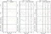 |
Fig. 2. Background-subtracted light curves of Haro 11 binned at 3.6 ks in the S + M and M + H bands (in counts; upper panels), along with the hardness ratios HR1 and HR2 (lower panels) defined by Eqs. (1) obtained from the XMM-Newton and Chandra source and background light curves using the Bayesian quadrature method of the BEHR. The light curves of the later observations were scaled up based on the instrument effective areas relative to the first one. The observation identifiers are given in the top panels. |
Figure 3 presents hardness ratio diagrams in which the hardness ratios HR1 and HR2 are plotted versus the light curves of the S + M and M + H bands binned at 3.6 ks, respectively. The hardness diagrams from the 2005 XMM observations show some patterns, but they are not strong enough to be associated with any spectral-state transition similar to those seen in BHB (see, e.g., Homan & Belloni 2005). However, we find statistically significant changes in the HR2 hardness ratio in the next subsection, which could be due to potential superwinds. Figure 2 shows that HR1 sometimes decreases with an increase in HR2. Moreover, the hardness ratio HR2 was occasionally lower when the source was softer and brighter (higher S + M and M + H). The HR2 diagram of X1 suggests the possibility of some transition patterns between the “faint/hard” and “bright/soft” spectral states. This might be related to a possible BHB, though the diagrams lack vigorous transition patterns. The hardness diagrams of X2 depict robust transitions, which are results of occasional increases in brightness (higher S + M and M + H) as seen in Fig. 2. Although the sources X1 and X2 cannot be separated in the XMM-Newton observations, the brightening incidents seen in the Chandra light curves suggest that both X1 and X2 could be responsible for the transient shapes created in the XMM-Newton hardness diagrams, while the X1 source emits more X-ray photons than X2.
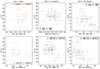 |
Fig. 3. Hardness ratio diagrams of Haro 11 made with XMM-Newton and Chandra observations. The hardness ratios HR1 (top) and HR2 (bottom) as defined by Eqs. (1) are plotted against the background-subtracted S + M and M + H bands (in counts), respectively, with a bin size of 3.6 ks. The hardness ratios and the corresponding 1-σ uncertainties were determined from the light curves of the source and background using the Bayesian quadrature method of the BEHR. The counts of the later observations were scaled up according to the instrument effective areas with respect to the first one. |
3.2. Statistical analysis of variability
To quantify variability, we analyzed the light curves and their corresponding hardness ratios using different statistical methods for homogeneity and normality.
To evaluate the homogeneity of time series, we calculated the von Neumann ratio defined as the mean squared successive difference with respect to the variance, η ≡ δ2/σ2 (von Neumann 1941),

where δ2 and σ2 are the mean squared successive difference and the variance of data points, respectively, n is the number of each data point, and N is the total number of data points. The mean von Neumann ratio is  for a normal distribution (Young 1941). We estimated the confidence levels on
  according to the statistically significant threshold of α = 0.05. The von Neumann ratio of time series within the confidence intervals of the normal von Neumann ratio implies homogeneity, whereas those outside the aforementioned intervals suggest inhomogeneity in successive time series.
To examine the normality of data points, we conducted three nonparametric statistical analyses of light curves, namely the Lilliefors test, the Anderson–Darling (AD) test, and the Shapiro–Wilk (SW) test. The Lilliefors test, which is an extension of the Kolmogorov–Smirnov (KS) approach, uses estimated mean μ and variance σ2 of the sample for the examination of a normal distribution 𝒩(μ, σ2). The KS test is suitable for the standard normal distribution 𝒩(0, 1). The Lilliefors test is based on the maximum difference between the empirical distribution function (EDF) of the sample and the cumulative distribution function (CDF) of the normal distribution (Lilliefors 1967):

where Fnorm(x) is the CDF of the normal distribution 𝒩(μ, σ2), and F(x) is the EDF of the sample. This test was conducted with the corresponding function from the Statsmodels package (Seabold & Perktold 2010). The AD test, which was also carried out with the relevant function from Statsmodels, is based on the weighted squared difference (A2) between the EDF and the CDF, giving more weight to the tails of the CDF (Anderson & Darling 1952):
![$$ \begin{aligned} A^2 = N \int _{-\infty }^{\infty } [F(x)-F_{\rm norm}(x)]^2 w_{\rm norm}(x) dF_{\rm norm}(x), \end{aligned} $$](/articles/aa/full_html/2024/09/aa49388-24/aa49388-24-eq6.gif)
where wnorm(x)≡[Fnorm(x)(1 − Fnorm(x))]−1 is the weighting function. The SW test, which was conducted with the corresponding function from the SciPy package (Virtanen et al. 2020), utilizes the order statistics (Shapiro & Wilk 1965):

where xn are the sorted data points (x1 < ⋯ < xn), μ is the mean of data points, and a = (a1, …, an) is the coefficient vector defined as  using the vector m = (m1, …, mn)T of the ordered values mn of the normal statistics and their covariance matrix V. For all three statistical methods, p-value ≤0.05 rejects the hypothesis of a normal distribution with significant statistics, whereas p-values between 0.05 and 0.1 are marginally significant for the null hypothesis. The SW was found to be the most effective method, followed by the AD and then Lilliefors (Stephens 1974; Razali & Wah 2011), though the AD is more powerful in the CDF with a sharp-edged peak and abruptly ending tails.
In addition, we employed the Gregory-Loredo (GL) algorithm to calculate the probability of a periodic signal, pper(ω) = Oper(ω)/[1 + Oper(ω)], according to the sum of odds ratios  , where the odds ratio Om1(ω) is defined by Eq. (5.25) in Gregory & Loredo (1992). For pper < 0.5, there is definitely no variable, while pper ≥ 0.9 is certainly variable. A light curve may be variable if 0.5 ≤ pper < 2/3, and is considered to be variable if 2/3 ≤ pper < 0.9.
Table 2 presents our results derived from the aforementioned statistical methods. It can be seen that the von Neumann ratios (η) suggest inhomogeneity only in successive data points of the S + M band for the XMM and CXO-X2 data, having η outside the confidence intervals of  . We also notice the absence of normality with a significant statistic in HR2 of the XMM data based on p-value ≤0.05 from all three methods. In addition, there could be no normality in the S + M light curve of the CXO-X1 observations with a marginally significant statistic according to p-value ≤0.1 from the Lilliefors test. The p-values derived for the rest of the data are consistent with normality. The GL probability results of the data indicate definitely variability in M + H of the XMM and CXO-X2 data. The S + M data of XMM, as well as CXO X1 and X2, are also considered to be variable according to the values of pper(ω). The M + H band in CXO X1 may be variable according to the GL probability outcome. However, we caution that the GL results could be less reliable due to the low number of data points.
Statistical tests of X-ray variability.
In summary, the spectral transition pattern seen in HR2 of the XMM data in Figure 3 is statistically significant according to normality tests, whereas hardness transitions are insignificant in other cases, apart from the marginal pattern in the S + M band in X1. Because the XMM observations cover both X1 and X2, we cannot determine the origin of such a spectral transition in HR2. Our analysis also yields p-values of around 0.2 and 0.1 with the AD and SW tests on HR2 of the CXO X2 data, respectively, as well as p-values around 0.1–0.2 using the Lilliefors test on HR1 of X2 and with all tests on HR1 of XMM. The p-values are all small, thus perhaps suggestive of possible hardness transitions. Moreover, the S + M light curves in XMM and CXO X2 do not appear to be homogeneous based on the von Neumann statistics, which again suggests the likelihood of nonrandom variations.
3.3. Principal component analysis
Principal component analysis (PCA) is a commonly used eigenvector-based approach for conducting multivariate statistics, which has been described in several books (e.g., Jolliffe 2002). It can be employed to disentangle different spectral features primarily contributing to the intricate source variability by decomposing the time-stacked data into a set of PCA components that are independent and variable, thus providing the degrees of variability with fractional contribution orders. It has been widely used in the field of astronomy as a valuable tool for multivariate research. Its application can be traced back to some works on the stellar spectral classification (Deeming 1964; Whitney 1983), followed by spectral studies of galaxies (Faber 1973; Bujarrabal et al. 1981; Efstathiou & Fall 1984), and UV data analyses of quasars (Mittaz et al. 1990; Francis et al. 1992), in addition to imaging spectroscopy of the ISM (Heyer & Schloerb 1997; Brunt et al. 2009). This approach has also been extensively used for spectral analyses of high-mass X-ray binaries (Malzac et al. 2006; Koljonen et al. 2013), AGNs (Miller et al. 2008; Parker et al. 2014a, 2017, 2018; Gallo et al. 2015), and blazar variability (Gallant et al. 2018).
PCA is a statistical technique that can split timing spectroscopic observations into sets of orthogonal spectral and temporal eigenvectors together with ordered eigenvalues of time variability. The process of projecting the time-stacked spectra onto the eigenvectors results in a series of diagnostic eigenvalues, which are associated with the variability contributions of ordered spectral sources resulting in the entire spectrum. We denote each paired decomposed spectral source and its time series as a principal component, identified by the order i = 1, 2, …, n, where n corresponds to the number of time slices in each dataset binned at m energy channels. The variability fractions in the data are described by the normalized eigenvalues. The determination of spectral components and their light curves involves the eigen-decomposition of an m × n matrix, containing spectroscopic data sliced at n time intervals and binned at m energy channels.
For our eigenvector multivariate analysis, we used a modified version of the PCA Python code developed by Parker et al. (2015) using the singular value decomposition (SVD; Press et al. 1997) function from the NumPy linear algebra (Harris et al. 2020). This program transfers the given n time-segmented PHA data into a rectangular array (m × n) consisting of a series of n spectral data binned within m energy channels, which is then decomposed using the SVD function into a 2D array (m × m) including PCA components Fm(E) sorted by their contribution orders, an n-array of eigenvalues associated with the variance of each PCA component, and a square matrix (n × n) containing eigenvectors providing the time-binned PCA light curves An(t). The PCA components and light curves represent the spectral shape and temporal change of the variable features present in a complex source, respectively. The determination of the fractional variability of each PCA component is achieved by dividing the corresponding eigenvalue by the sum of all eigenvalues. The method employed for calculating errors in the PCA program is based on the given spectra undergo random perturbations and SVD recalculations (see Miller et al. 2007).
To conduct PCA, we employed the reprocessed event of each XMM-Newton dataset to create the time-filtered events at time intervals of 10 ks using the SAS function evselect. The time-sliced event data similarly include the suitable patterned events and the PI channels appropriate for EPIC-pn and MOS2, in addition to the exclusion of the flaring background-affected events. The especget tool was utilized to generate time-stacked PHA files from the time-filtered events using the same source and background circular regions described in Sect. 2. For the Chandra ACIS-S observations, the event files were filtered at time stacks of 10 ks using the CIAO task dmcopy. The source and background spectra, as well as the corresponding response data, were made from the time-filtered events with the CIAO task specextract, set to correct point-like PSF in the ARF data. After the data reduction, we proceeded with supplying the time-sliced flux data of the source and background to the PCA program, in addition to the effective area data, which yielded the PCA components, time series, and normalized eigenvalues for each dataset. The effective area column Aeff(E) from the ARF was used to transfer the count value C(E) in each energy bin E to flux one F(E) according to F(E) = C(E)/(Aeff(E)t), where t is the exposure time. For each dataset, a mean spectrum, Fmean(E) was derived from the background-corrected PCA spectra, which was used to obtain the normalized PCA spectra as follows fk(E) = [Fk(E)−Fmean(E)]/Fmean(E).
Figure 4 presents the eigenvalue-fraction diagrams the XMM-Newton combined pn and MOS2, as well as the Chandra ACIS-S X1 and X2, in which the normalized eigenvalues of the principal components are plotted against the corresponding eigenvector orders. The number of nonzero eigenvalues is proportional to the number (n) of time-segmented PHA data in each dataset. These diagrams can be used to ascertain the statistical significance of the PCA components. The line in each diagram depicts the linear regression between logarithmic values of fractional variability and eigenvector orders, starting from three onward, which allows us to distinguish significant PCA components from those possibly created by noise fluctuations (see, e.g., Koljonen et al. 2013; Parker et al. 2015). Accordingly, the first two components in the XMM-Newton pn+MOS2 data and the Chandra X1, and the first component in Chandra X2 are expected to be statistically significant based on the eigenvalue-fraction diagrams.
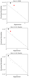 |
Fig. 4. Eigenvalue–fraction diagram of the XMM-Newton EPIC-pn+MOS2 (top), Chandra ACIS-S X1 (middle), and X2 (bottom). The normalized fraction variability values of PCA components are plotted against the corresponding eigenvector orders. The linear regression among logarithmic fractional eigenvalues starting from three onward is also plotted (gray line). The number of nonzero eigenvalues in each diagram corresponds to the number of time-sliced spectra. The spectra and time series of the PCA components (color circles), which are statistically significant, are plotted with the same colors in Figure 5. |
Figure 5 shows the PCA components and time series of the XMM-Newton pn+MOS2, as well as the Chandra ACIS-S X1 and X2. A series of peaks and troughs are seen in the principal components, which might correspond to variable emission and/or absorption features, possibly from ionized powerful superwinds. We see that these features are located at energies, where we could expect lines from H-like and He-like ions of different elements, such as S XV Heα 2.45 keV and Ca XX Lyα 4.11 keV as labeled in the plots. The respective light curves imply that the principal components are primarily linked to some brightness incidents happening during the observations (see Fig. 2). The orders higher than 2 are not statistically significant in XMM and X1, since they follow the linear regression line in Figure 4, so they do not seem to represent any spectral feature. We see that the second time series A2(t) of the Chandra X1 partially follows the trend in A1(t), so it might be associated with the features of a superwind. We should note that X1 could also contain a wide-angled bipolar outflow based on observations made with the Fibre Large Array Multi Element Spectrograph (FLAMES) on the VLT (James et al. 2013), which can explain the double spectral features of an outflow in PCA. Especially, the time series A2(t) of X1 also has a peak that is co-temporal with the peak in A1(t). This means that they could be related to some brightening incidents that occurred at the beginning of the 2006 observation.
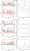 |
Fig. 5. Normalized PCA components fk(E) (left panels) of the XMM-Newton pn+MOS2 (top), Chandra ACIS-S X1 (middle), and X2 (bottom) of Haro 11, along with the corresponding time-binned light curves Ak(t) (right). The fractional percentage variability of each PCA component is also given in the left panel. The energies corresponding to the possible lines that arise from H-like and He-like ions are marked. |
Previously, Parker et al. (2017) exploited PCA to reexamine the existence of outflowing absorption lines in the X-ray variability of a narrow-line Seyfert 1 galaxy. As labeled in Fig. 5, the principal spectra may contain several emission and/or absorption lines from H-like and He-like ions of various elements, which could originate from the outflow similar to those identified in the UV observations of Haro 11 (Grimes et al. 2007; Hayes et al. 2016; Östlin et al. 2021; Komarova et al. 2024). Especially, some hydrodynamic simulations of starburst superwinds also predicted the formation of radiatively cooling expanding regions along with hot (106 − 8 K), X-ray-emitting layers, where the UV lines from highly ionized ionic species could be generated (Wünsch et al. 2017; Danehkar et al. 2021b, 2022). Recent hydrodynamic simulations conducted by Yu et al. (2021) demonstrated that H-like and He-like Kα emission lines from O, Mg, Si, S, Ar, Ca, and Fe ions could be produced in the X-rays of starburst outflows. Moreover, several H-like and He-like emission lines of O, Ne, Mg, Si, S, Ar, and Fe were detected in the X-ray observations of starburst-driven outflows in NGC 253 (Ptak et al. 1997; Bauer et al. 2007, 2008; Mitsuishi et al. 2013; Lopez et al. 2023) and M82 (Ptak et al. 1997; Ranalli et al. 2008; Liu et al. 2011; Lopez et al. 2020). However, the available low-count X-ray data of Haro 11 do not allow us to confirm the presence of H-like and He-like emission lines through spectral modeling.
3.4. Spectral analysis
To further evaluate the X-ray features of Haro 11, we used phenomenological models to reproduce the curvatures in the XMM-Newton and Chandra observations. To improve the fitting statistics, we modeled the soft excess (< 1.1 keV) using a (multi-)blackbody accretion disk spectrum, which might originate from either an AGN or BHB in X1, and the hard band (> 1.1 keV) using a power-law model, in addition to a line-of-sight absorbing column. Our spectral analysis was conducted using the Interactive Spectral Interpretation System (ISIS v 1.6.2-51; Houck & Denicola 2000), which provides access to several S-Lang libraries, as well as the spectral models included in the X-ray spectral fitting package XSPEC (v 12.13.0; Arnaud 1996) of the HEAsoft collection (v 6.31.1). The Simulated Annealing (SA) minimization algorithm (Corana et al. 1987), together with the “Cash” statistic (C-stat; Cash 1979), were used to model simultaneously all the background-subtracted Chandra/ACIS-S data. While the C-stat is the most effective method for the analysis of low-count data, the SA optimization method is also promising for extremely low counts, albeit with a highly intensive use of computing resources. We also simultaneously modeled the source and background data for each of the XMM-Newton dataset using the C-stat and SA method, with the background spectrum fitted by two broken power-law components. The source spectra, along with the corresponding spectral models, are shown in Figure 6.
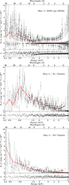 |
Fig. 6. XMM-Newton EPIC-pn+MOS2 (top), Chandra ACIS-S X1 (middle), and X2 (bottom) observations of Haro 11, along with the spectral models constant × phabs × (diskbb + zpowerlw) and constant × phabs × (zbbody + zpowerlw) (in red) fitted to the XMM-Newton and Chandra data, respectively. |
For the soft excess in the XMM data, a multicolor disk blackbody model (diskbb; see, e.g., Mitsuda et al. 1984; Zimmerman et al. 2005) was used, since they include both the X-ray sources X1 and X2. However, a simple blackbody model (zbbody) in the rest frame (z = 0.020598) was sufficient to describe the soft excesses of X1 and X2 observed by the Chandra ACIS-S. The power-law model (zpowerlw) that reproduces the hard excess has the two free parameters: photon index (Γ) and normalization factor (Kp). To recreate the drop (absorbed) pattern seen in the soft excess, an absorption component (phabs) was applied to both the soft and hard components, yielding the hydrogen column density (NH) of line-of-sight absorbing material. The spectral models, which were fitted to the 0.4–10 keV energy range of the XMM data and 0.4–8 keV of CXO as seen in Fig. 6, are as follows: constant × phabs × (diskbb + zpowerlw) for XMM and constant × phabs × (zbbody + zpowerlw) for CXO. The cross-normalization constant was set to the index number of each active dataset3, which allows data-dependent modeling of different epochs and instruments.
The best-fitting parameters of the spectral models are listed in Table 3. The ISIS standard procedure for confidence limits (conf_loop) was used to determine the best-fitting parametric values and the corresponding uncertainties at 90% confidence. One can note that the XMM-Newton data were slightly different (Γ ∼ 1.8) than the Chandra data, albeit consistent based on the confidence limits. The comparison of Chandra/ACIS-S and XMM-Newton model parameters indicates that the source X1 in the Chandra is more than 2 times more obscured than what is seen in the XMM, while the column density along the line of sight toward X2 is 10 times lower than that in X1. Figure 6 also shows that the soft excess (< 1 kev) in X2 is stronger than X1, which is suggestive of a much lower absorbing material in X2. Interestingly, the absorbing column for the XMM-Newton spectra, which are made up of both X1 and X2, are lower than that derived for X1 with the Chandra. The blackbody temperature and normalization in X2 are lower than those in X1. This means that the soft excess in the XMM-Newton data mostly originates from X1, where it is subject to the possible accretion associated with an AGN or a BHB. The power-law model describing the hard excess in the source X2 (Γ ∼ 2) is slightly harder than that derived for X1 (Γ ∼ 2.3). However, the power-law normalization scale for the X1 source is much higher than that in X2, meaning that X1 is also brighter in the hard excess (see Table 3).
Best-fitting parameters for the XSPEC models of the XMM-Newton EPIC-pn+MOS2, and Chandra/ACIS-S X1 and X2 data.
The previous study of the 2006 Chandra observation by Prestwich et al. (2015) using the aperture of 1.1″ also indicated that X2 is much softer and slightly less obscured than X1, while X1 is twice as luminous as X2, which is similar to our finding in Table 3. Moreover, a recent analysis of the stacked Chandra/ACIS-S data by Gross et al. (2021) with the extraction radius of 1.7″ implied that X1 could also have an absorbing column that is four times higher than that of X2. The power-law photon index (Γ ∼ 2) we derived for X2 is in reasonable agreement with that found by Gross et al. (2021), though our best-fitting parameter values for X1 are slightly different. This discrepancy could be explained by our approach of simultaneously fitting a spectral model to all the spectra rather than using a stacked spectrum.
In Table 3, we also list the unabsorbed X-ray flux (FX) and the X-ray luminosity (LX) at D = 82 Mpc. The flux of each model, in addition to the luminosity, were derived over the energy range 0.4–8 keV using an S-Lang flux calculation routine (model_flux) from the custom ISIS functions (distributed by M. Nowak)4. The confidence levels of the X-ray fluxes and luminosities are based on the those derived from the power-law normalization factors. The high uncertainties could be related to the X-ray variability and low counts. One can note that the source X1 is twice as bright as X2. We also see that the X-ray luminosity in the XMM-Newton EPIC-pn is roughly equal to the luminosity sum of the sources X1 and X2 collected by the Chandra ACIS-S. Our X-ray luminosity estimation for the source X2 (LX ∼ 4 × 1040 erg s−1) agrees approximately with the ULX luminosity (LX ∼ 5–6 × 1040 erg s−1) derived by Gross et al. (2021), albeit with D = 84 Mpc. Moreover, we obtained an X-ray luminosity for X1 (LX ∼ 9 × 1040 erg s−1) similar to the extremely hard X-ray luminosity (LX ∼ 1041 erg s−1) found previously (Prestwich et al. 2015; Gross et al. 2021).
3.5. Simulations
To assess the feasibility of PCA-suggested lines, we simulated spectra for XMM-Newton/EPIC-pn and Chandra/ACIS-S by adopting the total exposures of all combined XMM-Newton and Chandra data, respectively. Our simulations were conducted with the ISIS function fakeit using the RMF and ARF of the XMM-Newton/EPIC-pn in 2004 and the Chandra/ACIS-S data collected in 2006. We used the same spectral models of Sect. 3.4, but included the XSPEC models zgauss to simulate possible features of emission lines, namely constant × phabs × (diskbb + zpowerlw + ∑ zgauss) for XMM-pn and constant × phabs × (zbbody + zpowerlw + ∑ zgauss) for CXO-X1/X2 (see Fig. 7). We set the model parameters to those values determined from our spectral analysis. The energy-independent factor in the XSPEC component constant of each spectral model was adjusted to reproduce exactly the same source count given in Table 3. We shifted the zgauss components with an outflow velocity of vout = −290 km s−1 in the rest frame according to the absorption lines blueshifted with 200–380 km s−1 detected in the UV observations collected with the Far Ultraviolet Spectroscopic Explorer (FUSE) and the Cosmic Origins Spectrograph (COS) on the HST (Grimes et al. 2007; Hayes et al. 2016), and assumed a Gaussian RMS width of σ = 10 eV.
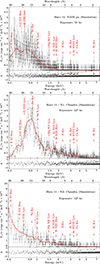 |
Fig. 7. Simulated spectra of the XMM-Newton EPIC-pn (91 ks) and Chandra ACIS-S X1 and X2 sources (127 ks) using the model parameters listed in Table 3, including the emission lines suggested by our PCA, as labeled in Fig. 5. |
The normalization factors (K) of the zgauss functions were iteratively modified to reproduce similar features seen in the observed spectra. Table 4 presents the aforementioned factors adopted for the zgauss models in the simulated spectra, which may be served as the upper limits to the emission lines possibly presented in the actual observations. Although it is difficult to distinguish any lines below 1 keV and above 3 keV, our simulated spectra suggest the possible presence of the blueshifted emission lines Mg XII Lyα 1.471 keV, Al XIII Lyα 1.727 keV, Si XIII Heα 1.865 keV, and S Kα 2.308 keV in the XMM and CXO-X1 data as seen in Figure 7. In the case of CXO-X2 with extremely low photons, some features seen in the observation resemble the blueshifted lines Mg XII Lyα 1.471 keV and Si XIII Heα 1.865 keV. Our simulations indicate that the aforementioned emission lines in the medium band (1.1–2.6 keV), if they are genuinely present, can be constrained using observations taken with an exposure of at least 300 ks, which result in 3209, 3119, and 1034 counts in XMM-pn (0.4–10 keV), CXO-X1 and -X2 (0.4–8 keV), respectively.
To see the effects of the line variability, we employed the same aforementioned spectral models to generate simulated 10 ks-stacked XMM-Newton spectra, but with moderately variable normalization factors in the model components. Our approach is similar to the method used by Parker et al. (2014b), albeit with the Gaussian function heights tied to the amplitudes of the PCA time series extracted from the observations. To create the variable emission-line fluxes, we simply set the normalization factors of the XSPEC functions zgauss to [1 + (A1(t)+A2(t))/2]×K, where K is the value chosen from Table 3, and A1(t) and A2(t) are the PCA time series derived from the XMM-Newton observations plotted in Fig. 5. However, we caution that our assumption of uniform changes in the emission-line fluxes may not be physically correct due to the presence of different stratification ionization zones in an ionized outflow. To emulate the background noise, we added 2% variation to the normalization factors of the XSPEC models diskbb and zpowerlw using variable random seeds with a normal distribution. The simulated spectra were created with the ISIS function fakeit with an interval exposure of 10 ks using the RMF and ARF of the XMM-Newton/EPIC-pn data, and were written to PHA files with the help of the Remeis ISIS functions (ISISscripts). We again loaded and decomposed them into principal components using the SVD function in the same Python program used for our PCA of the observations.
Figure 8 shows the statistically significant PCA components derived from our simulated spectra with variable emission-line fluxes. It can be seen that variable emission-line fluxes in the spectral model produce a series of high and low points in the PCA spectra. Interestingly, the homogeneous variation in line fluxes, which could be linked to a varying ionization parameter of an ionized outflow, results in two PCA components roughly similar to those seen in Fig. 5. We should note that the features we see in the PCA components derived from the observations may not be associated with a single outflow. However, our simulation with a simple assumption supports the idea that varying fluxes in emission lines, likely from different stratification layers of superwinds, might be present in Haro 11.
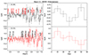 |
Fig. 8. Normalized PCA components fk(E) and the corresponding time series Ak(t) of the simulated XMM-Newton EPIC-pn spectra segmented at 10 ks with the model parameters listed in Table 3, including the zgauss models of the emission lines given in Table 3 with variable normalization factors as described in text. |
4. Discussions
4.1. Multiphase ionized superwinds in Haro 11
We analyzed the X-ray variability of the starburst knots B (X1) and C (X2) of Haro 11 using the hardness diagrams and eigenvector-based multivariate statistics. There are some hourly transient incidents in both sources seen in the hardness ratios, which may be associated with emission features from ionized superwinds according to the PCA components derived from the X-ray observations.
The signature of ionized superwinds in Haro 11 has been seen in UV observations. The possible X-ray outflows could be counterparts to the O VIλλ1032,1038 emission found in HST imaging (Hayes et al. 2016), in addition to an O VI-absorbing component blueshifted with velocities of 200–380 km s−1 detected in the FUSE and HST/COS UV spectroscopic observations (Grimes et al. 2007; Hayes et al. 2016). Broad, low-ionization interstellar absorption lines were also seen in the FUSE observations (Grimes et al. 2007), which are often observed in UV observations of LBGs (Shapley et al. 2003). The blueshifted O VI absorption line implies the presence of ionized outflows similar to those seen in high-z LBGs. The blueshifted UV absorption Si II and Si IV lines were also identified in the FUSE data, suggesting the presence of multiphase outflows with velocities extended to 500 km s−1 within the neutral ISM (Östlin et al. 2021). This can create shock-ionization, which may result in blueshifted emission lines in X-rays.
In addition, Grimes et al. (2007) speculated whether the O VI emission in Haro 11 originates from radiative cooling or resonance scattering, while also suggested that a significant amount (20%) of the supernova feedback could be lost owing to radiative cooling. Recently, some hydrodynamic simulations put forward the production of C IVλ1550 and O VIλ1037 emission via nonequilibrium ionization within radiatively cooling superwinds (Gray et al. 2019; Danehkar et al. 2022). Interestingly, Knot A in Mrk 71, which is the nearest LyC emitter candidate, also exhibits diffuse C IVλ1550 emission with a remarkable link to catastrophic radiative cooling based on nonequilibrium computations (Oey et al. 2023). The detection of C IV associated with radiative cooling in Knot C (X2) in Haro 11 requires deeper spatially resolved UV observations, in addition to high-resolution X-ray spectroscopy.
The evidence for superwinds in Haro 11 is not limited to those seen in UV observations and is also visible in spatially resolved optical observations. Knot B (X1) seems to be the main source for fast outflows, with escape wind speeds ranging from 240 to 600 km s−1, according to integral field unit (IFU) observations made with the optical VLT/MUSE instrument (Menacho et al. 2019). An apparently broad component blueshifted at 400 km s−1 was also identified in the MUSE data, which was interpreted as ionized outflows away from knots B and C (Sirressi et al. 2022). Moreover, Sirressi et al. (2022) argued that Knot C is a depleted area formed by a previous outflow, as suggested by Menacho et al. (2019), while the outflow in Knot B seems to be young and less developed. Previously, Hayes et al. (2007) also found evidence for a bipolar morphological outflow in Knot C based on the Lyα image. Moreover, a wide-angled bipolar outflow centered on Knot B was also proposed by James et al. (2013) based on optical IFU observations made with VLT/FLAMES.
Numerical simulations demonstrated that the propagation of powerful outflows into the surrounding ISM results in multiphase stratified zones via collisional ionization, which leave observable imprints in X-rays (Yu et al. 2021), in addition to optical and UV lines (Danehkar et al. 2021b). In particular, X-ray spectra of starburst-driven outflows in NGC 253 and M82 showed several emission lines of various elements (Liu et al. 2011; Mitsuishi et al. 2013; Lopez et al. 2020, 2023). As discussed by Menacho et al. (2019), such a strong highly ionized outflow is capable of clearing galactic channels, which allows the escape of LyC radiation in Knot C (X2).
4.2. Covering fractions and densities in X1 and X2
Our spectral analysis of X1 and X2 based on the Chandra ACIS-S data implies that X2 is less covered by the absorbing material than X1. The ISM around X2 could have lower column densities or some low-density channels, which would make it optically thin to the LyC radiation. In particular, the source X2, which is overall fainter in X-rays compared to X1, has a Lyα escape fraction of 6%, whereas the escape fraction of Lyα in X1 was estimated to be ≲1% (Östlin et al. 2021). This is consistent with the escape fractions of 3.4% and 5.1% in X1 and X2, respectively, determined from the leaking LyC luminosities in 903–912 Å (Komarova et al. 2024).
The narrow Lyα emission with no broad absorption recently seen with FUSE and HST/COS, along with the Si II line profiles, hinted at a low (≲50%) covering fraction of neutral gas in X2 (Östlin et al. 2021). However, Rivera-Thorsen et al. (2017) deduced that the surrounding ISM around the knots is most likely either a clumpy density-bounded neutral medium or an ionization-bounded neutral medium within a highly ionized clumpy medium with an overall covering fraction of unity using the apparent optical depth method. They also suggested that the LyC escape might occur if the proportion of dense gas covering X2 is partly low enough. This necessitates that stellar feedback should significantly contribute to clearing pathways partially in X2 for ionizing radiation to penetrate the neutral medium. Previously, Sandberg et al. (2013) also concluded high optical depths but a low covering fraction (∼10%) in all the knots through the spatially resolved observations of the sodium doublet (Na D) profiles.
Optical IFU spectroscopy of Haro 11 with the VLT/MUSE studied by Menacho et al. (2021) revealed that the ISM around X2 is less dense (≲35 cm−3), hotter (≳16 900 K), and less metallic (12+log O/H ∼ 7.46) than X1 (∼390 cm−3, ∼9600 K, and 12+log O/H ∼ 8.55). Using the IFU FLAMES on the VLT, James et al. (2013) also derived the same results: ne = 150 cm−3, Te = 16 600 K, and 12+log O/H = 7.8 for the ISM in Knot C (X2); and ne = 370 cm−3, Te = 12 100 K, and 12+log O/H = 8.25 in Knot B (X1). The LyC radiation and hot gaseous outflows are probably escaping through low-density channels in X2. Using the VLT/MUSE observations, Menacho et al. (2019) also found evidence for a fragmented, kiloparsec-scale superbubble shell around X2, which could be created by a past powerful superwind. This is supplemental to a low-density and high-temperature medium present in X2. Low-density channels and broken shells in the ISM surrounding X2, which might be created by powerful outbursts, could play a leading role in facilitating the escape of LyC and Lyα photons. In the future, if absorption lines are robustly constrained by high-resolution X-ray observations (e.g., XRISM), it will be possible to measure the outflow velocities in addition to the line equivalent widths (i.e., the column densities of ions produced in X-ray outflows).
5. Conclusion
In this paper we have analyzed the 2004 and 2005 XMM-Newton (EPIC-pn: 31.3 ks and MOS2: 59.9 ks) and Chandra/ACIS-S (127.3 ks; see Table 1) observations of the Lyman break analog Haro 11. We used hardness-intensity diagrams to search for any possible spectral-state transition. We utilized principal component statistics to determine the spectral feature that is responsible for X-ray variability. We also conducted spectral modeling to reproduce the continua using a (multi-)blackbody spectrum and a power-law component covered by a line-of-sight absorbing column, in addition to the simulations of PCA-suggested lines. Our key findings are summarized as follows:
(i) Our timing analysis depicts some stochastically increases in the hardness ratios over the course of the observations (see Fig. 2), which might be associated with the variability of emission lines made by ionized superwinds, as evidenced by the PCA light curves (Fig. 5). Although the brightening incidents originate from both X1 and X2, the source X1 seems to contribute significantly higher counts to the X-ray variability.
(ii) Our statistical analysis indicates that the variability in the HR2 hardness ratio of the XMM data is statistically significant according to all three normality tests (see Table 2). In addition, the von Neumann statistics imply inhomogeneous changes in the S + M light curves of the XMM observations. Moreover, the Lilliefors test shows marginally significant variations in the S + M band of X1.
(iii) Our eigenvector-based multivariate analyses of the XMM-Newton/EPIC-pn+MOS2 data and the Chandra/ACIS-S data of X1 and X2 indicate that the principal components responsible for the X-ray variability contain some peaks and valleys, which could be related to the emission lines from the starburst-driven outflow, similar to those detected in the UV observations (Grimes et al. 2007; Hayes et al. 2016; Östlin et al. 2021; Komarova et al. 2024). Particularly, H-like and He-like emission lines of several elements, such as O, Mg, Si, S, Ar, and Fe, were detected in the X-ray spectra of starburst outflows in NGC 253 (Bauer et al. 2007; Mitsuishi et al. 2013; Lopez et al. 2023) and M82 (Ranalli et al. 2008; Liu et al. 2011; Lopez et al. 2020), and also predicted by hydrodynamic simulations of starburst galaxies (Yu et al. 2021). The presence of highly ionized emission lines in Haro 11 should be confirmed by deeper high-spectral-resolution X-ray spectroscopic observations in the future. Additionally, our PCA of the XMM and CXO-X1 data revealed a second principal component that has a deviation from the noise-related regression (see Fig. 4). We see that the light curve A2(t) of X1 partially treads on the heels of A1(t) (see Fig. 5), and both may have a connection to the same brightening incidents seen in the 2006 observation. This component might correspond to the spectral features of either another outflow or the opposite part of an extended bipolar outflow. Interestingly, James et al. (2013) suggested the presence of a wide-angled bipolar outflow in X1 based on spatially resolved IFU observations. Alternatively, as our simulation suggests, an outflow with a varying ionizing source could also result in two PCA components (see Fig. 8).
(iv) The time-averaged models of the Chandra/ACIS-S spectra (see Table 3) suggest that the absorbing column in X2 (∼1.2 × 1021 cm−2) is much smaller than that in X1 (∼11.5 × 1021 cm−2). Our findings indicate that the ISM around X2 (which has the higher LyC leakage) has either a lower covering fraction or a lower column density, which may be the result of a strong superwind. Our spectral analysis also shows that X2 is slightly harder (Γ ∼ 2) and twice fainter (LX ∼ 4 × 1040 erg s−1) than X1 (Γ ∼ 2.3 and LX ∼ 9 × 1040 erg s−1). Moreover, our spectral modeling of the XMM-Newton data, which includes both X1 and X2, supports the presence of absorbing material (∼4.3 × 1021 cm−2).
(v) The simulated spectra, based on our spectral models, suggest the presence of some blueshifted emission lines, such as Mg XII Lyα 1.471 keV and Si XIII Heα 1.865 keV, in X1 and X2, which could originate from ionized superwinds driven by SSCs in Knots B and C. If these lines truly exist, they can only be constrained using observations much deeper than the currently available data. Our simulated spectra with varying emission-line fluxes, which could be produced by different ionization zones of an ionized superwind, also result in the PCA spectra resembling those derived from our analysis of the observations.
X-ray studies of Haro 11 would greatly improve our understanding of the underlying physics behind the LyC and Lyα leakage in high-z star-forming galaxies. In particular, radiation escaping from starburst galaxies in the early Universe is believed to significantly contribute to cosmic reionization (Cowie et al. 2009; Robertson et al. 2015; Mitra et al. 2015). Haro 11 can serve as a prominent local analog of LyC emitters. The use of future high-spectral-resolution X-ray missions such as XRISM (Tashiro et al. 2020) has the potential to provide further detailed information on the X-ray characteristics of Haro 11 and the physical phenomena that facilitated the escape of ionizing radiation from starburst galaxies during the reionization epoch.
Acknowledgments
We thank the anonymous referee for helpful suggestions that improved this paper, as well as Angela Adamo for useful discussions. A.D. acknowledges support from the NASA ADAP grant 80NSSC22K0626 and GSFC award 80NSSC23K1098. S.S. acknowledges the support provided by CONAHCyT México through the research grant A1-S-28458. Based on observations obtained with XMM-Newton, an ESA science mission with instruments and contributions directly funded by ESA Member States and NASA, observations made by the Chandra X-ray Observatory (CXO), and observations made with the NASA/ESA Hubble Space Telescope obtained from the Space Telescope Science Institute. This research has made use of software provided by the Chandra X-ray Center in the application packages CIAO and Sherpa, a collection of ISIS functions (ISISscripts) provided by ECAP/Remeis observatory and MIT, and Astropy, a community-developed core Python package for Astronomy (Astropy Collaboration 2013).
References
- Adamo, A., Östlin, G., Zackrisson, E., et al. 2010, MNRAS, 407, 870 [NASA ADS] [CrossRef] [Google Scholar]
- Anderson, T. W., & Darling, D. A. 1952, Ann. Math. Stat., 23, 193 [Google Scholar]
- Arnaud, K. A. 1996, ASP Conf. Ser., 101, 17 [Google Scholar]
- Astropy Collaboration (Robitaille, T. P., et al.) 2013, A&A, 558, A33 [NASA ADS] [CrossRef] [EDP Sciences] [Google Scholar]
- Barkana, R., & Loeb, A. 2001, Phys. Rep., 349, 125 [NASA ADS] [CrossRef] [Google Scholar]
- Basu-Zych, A. R., Lehmer, B. D., Hornschemeier, A. E., et al. 2013, ApJ, 762, 45 [NASA ADS] [CrossRef] [Google Scholar]
- Bauer, M., Pietsch, W., Trinchieri, G., et al. 2007, A&A, 467, 979 [NASA ADS] [CrossRef] [EDP Sciences] [Google Scholar]
- Bauer, M., Pietsch, W., Trinchieri, G., et al. 2008, A&A, 489, 1029 [NASA ADS] [CrossRef] [EDP Sciences] [Google Scholar]
- Bergvall, N., Masegosa, J., Östlin, G., & Cernicharo, J. 2000, A&A, 359, 41 [NASA ADS] [Google Scholar]
- Bergvall, N., Zackrisson, E., Andersson, B. G., et al. 2006, A&A, 448, 513 [NASA ADS] [CrossRef] [EDP Sciences] [Google Scholar]
- Boissay-Malaquin, R., Danehkar, A., Marshall, H. L., & Nowak, M. A. 2019, ApJ, 873, 29 [NASA ADS] [CrossRef] [Google Scholar]
- Brunt, C. M., Heyer, M. H., & Mac Low, M. M. 2009, A&A, 504, 883 [NASA ADS] [CrossRef] [EDP Sciences] [Google Scholar]
- Bujarrabal, V., Guibert, J., & Balkowski, C. 1981, A&A, 104, 1 [NASA ADS] [Google Scholar]
- Cash, W. 1979, ApJ, 228, 939 [Google Scholar]
- Corana, A., Marchesi, M., Martini, C., & Ridella, S. 1987, ACM Trans. Math. Softw., 13, 262 [CrossRef] [Google Scholar]
- Cormier, D., Lebouteiller, V., Madden, S. C., et al. 2012, A&A, 548, A20 [NASA ADS] [CrossRef] [EDP Sciences] [Google Scholar]
- Cowie, L. L., Barger, A. J., & Trouille, L. 2009, ApJ, 692, 1476 [NASA ADS] [CrossRef] [Google Scholar]
- Cowie, L. L., Barger, A. J., & Hasinger, G. 2012, ApJ, 748, 50 [CrossRef] [Google Scholar]
- Danehkar, A., Nowak, M. A., Lee, J. C., et al. 2018, ApJ, 853, 165 [NASA ADS] [CrossRef] [Google Scholar]
- Danehkar, A., Karovska, M., Drake, J. J., & Kashyap, V. L. 2021a, MNRAS, 500, 4801 [Google Scholar]
- Danehkar, A., Oey, M. S., & Gray, W. J. 2021b, ApJ, 921, 91 [NASA ADS] [CrossRef] [Google Scholar]
- Danehkar, A., Oey, M. S., & Gray, W. J. 2022, ApJ, 937, 68 [NASA ADS] [CrossRef] [Google Scholar]
- Dayal, P., & Ferrara, A. 2018, Phys. Rep., 780, 1 [Google Scholar]
- Deeming, T. J. 1964, MNRAS, 127, 493 [NASA ADS] [Google Scholar]
- Efstathiou, G., & Fall, S. M. 1984, MNRAS, 206, 453 [NASA ADS] [Google Scholar]
- Faber, S. M. 1973, ApJ, 179, 731 [NASA ADS] [CrossRef] [Google Scholar]
- Finoguenov, A., & Jones, C. 2002, ApJ, 574, 754 [CrossRef] [Google Scholar]
- Francis, P. J., Hewett, P. C., Foltz, C. B., & Chaffee, F. H. 1992, ApJ, 398, 476 [NASA ADS] [CrossRef] [Google Scholar]
- Fruscione, A., McDowell, J. C., Allen, G. E., et al. 2006, Proc. SPIE Conf. Ser., 6270, 62701V [NASA ADS] [CrossRef] [Google Scholar]
- Gabriel, C., Denby, M., Fyfe, D. J., et al. 2004, ASP Conf. Ser., 314, 759 [Google Scholar]
- Gallant, D., Gallo, L. C., & Parker, M. L. 2018, MNRAS, 480, 1999 [NASA ADS] [CrossRef] [Google Scholar]
- Gallo, L. C., Wilkins, D. R., Bonson, K., et al. 2015, MNRAS, 446, 633 [NASA ADS] [CrossRef] [Google Scholar]
- Garmire, G. P., Bautz, M. W., Ford, P. G., Nousek, J. A., & Ricker, G. R., Jr. 2003, Proc. SPIE Conf. Ser., 4851, 28 [NASA ADS] [CrossRef] [Google Scholar]
- Gray, W. J., Oey, M. S., Silich, S., & Scannapieco, E. 2019, ApJ, 887, 161 [NASA ADS] [CrossRef] [Google Scholar]
- Gregory, P. C., & Loredo, T. J. 1992, ApJ, 398, 146 [NASA ADS] [CrossRef] [Google Scholar]
- Grimes, J. P., Heckman, T., Strickland, D., et al. 2007, ApJ, 668, 891 [NASA ADS] [CrossRef] [Google Scholar]
- Gross, A. C., Prestwich, A., & Kaaret, P. 2021, MNRAS, 505, 610 [NASA ADS] [CrossRef] [Google Scholar]
- Harris, C. R., Millman, K. J., van der Walt, S. J., et al. 2020, Nature, 585, 357 [NASA ADS] [CrossRef] [Google Scholar]
- Hayes, M., Östlin, G., Atek, H., et al. 2007, MNRAS, 382, 1465 [NASA ADS] [Google Scholar]
- Hayes, M., Melinder, J., Östlin, G., et al. 2016, ApJ, 828, 49 [NASA ADS] [Google Scholar]
- Heil, L. M., & Vaughan, S. 2010, MNRAS, 405, L86 [NASA ADS] [CrossRef] [Google Scholar]
- Heyer, M. H., & Schloerb, F. P. 1997, ApJ, 475, 173 [NASA ADS] [CrossRef] [Google Scholar]
- Homan, J., & Belloni, T. 2005, Ap&SS, 300, 107 [Google Scholar]
- Houck, J. C., & Denicola, L. A. 2000, ASP Conf. Ser., 216, 591 [Google Scholar]
- James, B. L., Tsamis, Y. G., Walsh, J. R., Barlow, M. J., & Westmoquette, M. S. 2013, MNRAS, 430, 2097 [NASA ADS] [CrossRef] [Google Scholar]
- Jansen, F., Lumb, D., Altieri, B., et al. 2001, A&A, 365, L1 [NASA ADS] [CrossRef] [EDP Sciences] [Google Scholar]
- Jolliffe, I. T. 2002, Principal Component Analysis (Berlin: Springer) [Google Scholar]
- Koljonen, K. I. I., McCollough, M. L., Hannikainen, D. C., & Droulans, R. 2013, MNRAS, 429, 1173 [NASA ADS] [CrossRef] [Google Scholar]
- Komarova, L., Oey, M. S., Hernandez, S., et al. 2024, ApJ, 967, 117 [Google Scholar]
- Kosec, P., Pinto, C., Walton, D. J., et al. 2018, MNRAS, 479, 3978 [NASA ADS] [Google Scholar]
- Laird, E. S., Nandra, K., Hobbs, A., & Steidel, C. C. 2006, MNRAS, 373, 217 [NASA ADS] [CrossRef] [Google Scholar]
- Lehmer, B. D., Brandt, W. N., Alexander, D. M., et al. 2005, AJ, 129, 1 [Google Scholar]
- Leitet, E., Bergvall, N., Piskunov, N., & Andersson, B. G. 2011, A&A, 532, A107 [NASA ADS] [CrossRef] [EDP Sciences] [Google Scholar]
- Lilliefors, H. W. 1967, J. Am. Stat. Assoc., 62, 399 [CrossRef] [Google Scholar]
- Liu, J., Mao, S., & Wang, Q. D. 2011, MNRAS, 415, L64 [NASA ADS] [CrossRef] [Google Scholar]
- Lopez, L. A., Mathur, S., Nguyen, D. D., Thompson, T. A., & Olivier, G. M. 2020, ApJ, 904, 152 [Google Scholar]
- Lopez, S., Lopez, L. A., Nguyen, D. D., et al. 2023, ApJ, 942, 108 [NASA ADS] [CrossRef] [Google Scholar]
- Madden, S. C., Rémy-Ruyer, A., Galametz, M., et al. 2013, PASP, 125, 600 [NASA ADS] [CrossRef] [Google Scholar]
- Malzac, J., Petrucci, P. O., Jourdain, E., et al. 2006, A&A, 448, 1125 [NASA ADS] [CrossRef] [EDP Sciences] [Google Scholar]
- Menacho, V., Östlin, G., Bik, A., et al. 2019, MNRAS, 487, 3183 [CrossRef] [Google Scholar]
- Menacho, V., Östlin, G., Bik, A., et al. 2021, MNRAS, 506, 1777 [NASA ADS] [CrossRef] [Google Scholar]
- Micheva, G., Zackrisson, E., Östlin, G., Bergvall, N., & Pursimo, T. 2010, MNRAS, 405, 1203 [NASA ADS] [Google Scholar]
- Miller, L., Turner, T. J., Reeves, J. N., et al. 2007, A&A, 463, 131 [NASA ADS] [CrossRef] [EDP Sciences] [Google Scholar]
- Miller, L., Turner, T. J., & Reeves, J. N. 2008, A&A, 483, 437 [NASA ADS] [CrossRef] [EDP Sciences] [Google Scholar]
- Mitra, S., Choudhury, T. R., & Ferrara, A. 2015, MNRAS, 454, L76 [NASA ADS] [CrossRef] [Google Scholar]
- Mitsuda, K., Inoue, H., Koyama, K., et al. 1984, PASJ, 36, 741 [NASA ADS] [Google Scholar]
- Mitsuishi, I., Yamasaki, N. Y., & Takei, Y. 2013, PASJ, 65, 44 [CrossRef] [Google Scholar]
- Mittaz, J. P. D., Penston, M. V., & Snijders, M. A. J. 1990, MNRAS, 242, 370 [NASA ADS] [CrossRef] [Google Scholar]
- Nandra, K., Mushotzky, R. F., Arnaud, K., et al. 2002, ApJ, 576, 625 [CrossRef] [Google Scholar]
- Oey, M. S., Sawant, A. N., Danehkar, A., et al. 2023, ApJ, 958, L10 [NASA ADS] [CrossRef] [Google Scholar]
- Östlin, G., Hayes, M., Kunth, D., et al. 2009, AJ, 138, 923 [NASA ADS] [CrossRef] [Google Scholar]
- Östlin, G., Marquart, T., Cumming, R. J., et al. 2015, A&A, 583, A55 [NASA ADS] [CrossRef] [EDP Sciences] [Google Scholar]
- Östlin, G., Rivera-Thorsen, T. E., Menacho, V., et al. 2021, ApJ, 912, 155 [CrossRef] [Google Scholar]
- Park, T., Kashyap, V. L., Siemiginowska, A., et al. 2006, ApJ, 652, 610 [Google Scholar]
- Parker, M. L., Marinucci, A., Brenneman, L., et al. 2014a, MNRAS, 437, 721 [CrossRef] [Google Scholar]
- Parker, M. L., Walton, D. J., Fabian, A. C., & Risaliti, G. 2014b, MNRAS, 441, 1817 [CrossRef] [Google Scholar]
- Parker, M. L., Fabian, A. C., Matt, G., et al. 2015, MNRAS, 447, 72 [NASA ADS] [CrossRef] [Google Scholar]
- Parker, M. L., Alston, W. N., Buisson, D. J. K., et al. 2017, MNRAS, 469, 1553 [NASA ADS] [CrossRef] [Google Scholar]
- Parker, M. L., Reeves, J. N., Matzeu, G. A., Buisson, D. J. K., & Fabian, A. C. 2018, MNRAS, 474, 108 [Google Scholar]
- Pinto, C., Alston, W., Soria, R., et al. 2017, MNRAS, 468, 2865 [Google Scholar]
- Press, W. H., Teukolsky, S. A., Vetterling, W. T., & Flannery, B. P. 1997, Numerical Recipes in Fortran 77. The Art of Scientific Computing, 2nd edn. (Cambridge: Cambridge University Press), 1 [Google Scholar]
- Prestwich, A. H., Irwin, J. A., Kilgard, R. E., et al. 2003, ApJ, 595, 719 [Google Scholar]
- Prestwich, A. H., Jackson, F., Kaaret, P., et al. 2015, ApJ, 812, 166 [NASA ADS] [CrossRef] [Google Scholar]
- Ptak, A., Serlemitsos, P., Yaqoob, T., Mushotzky, R., & Tsuru, T. 1997, AJ, 113, 1286 [NASA ADS] [CrossRef] [Google Scholar]
- Ranalli, P., Comastri, A., Origlia, L., & Maiolino, R. 2008, MNRAS, 386, 1464 [CrossRef] [Google Scholar]
- Razali, N., & Wah, Y. B. 2011, J. Stat. Modeling Anal., 2, 21 [Google Scholar]
- Rivera-Thorsen, T. E., Östlin, G., Hayes, M., & Puschnig, J. 2017, ApJ, 837, 29 [NASA ADS] [CrossRef] [Google Scholar]
- Robertson, B. E., Ellis, R. S., Dunlop, J. S., McLure, R. J., & Stark, D. P. 2010, Nature, 468, 49 [Google Scholar]
- Robertson, B. E., Ellis, R. S., Furlanetto, S. R., & Dunlop, J. S. 2015, ApJ, 802, L19 [Google Scholar]
- Sandberg, A., Östlin, G., Hayes, M., et al. 2013, A&A, 552, A95 [NASA ADS] [CrossRef] [EDP Sciences] [Google Scholar]
- Seabold, S., & Perktold, J. 2010, Proc. 9th Python Sci. Conf., 57, 92 [CrossRef] [Google Scholar]
- Shapiro, S. S., & Wilk, M. B. 1965, Biometrika, 52, 591 [Google Scholar]
- Shapley, A. E., Steidel, C. C., Pettini, M., & Adelberger, K. L. 2003, ApJ, 588, 65 [Google Scholar]
- Sirressi, M., Adamo, A., Hayes, M., et al. 2022, MNRAS, 510, 4819 [NASA ADS] [CrossRef] [Google Scholar]
- Soria, R., & Wu, K. 2003, A&A, 410, 53 [NASA ADS] [CrossRef] [EDP Sciences] [Google Scholar]
- Stephens, M. A. 1974, J. Am. Stat. Assoc., 69, 730 [CrossRef] [Google Scholar]
- Strüder, L., Briel, U., Dennerl, K., et al. 2001, A&A, 365, L18 [Google Scholar]
- Tashiro, M., Maejima, H., Toda, K., et al. 2020, Proc. SPIE Conf. Ser., 11444, 1144422 [NASA ADS] [Google Scholar]
- Turner, M. J. L., Abbey, A., Arnaud, M., et al. 2001, A&A, 365, L27 [CrossRef] [EDP Sciences] [Google Scholar]
- Virtanen, P., Gommers, R., Oliphant, T. E., et al. 2020, Nat. Meth., 17, 261 [Google Scholar]
- von Neumann, J. 1941, Ann. Math. Stat., 12, 367 [Google Scholar]
- Weisskopf, M. C., Tananbaum, H. D., Van Speybroeck, L. P., & O’Dell, S. L. 2000, Proc. SPIE Conf. Ser., 4012, 2 [Google Scholar]
- Weisskopf, M. C., Brinkman, B., Canizares, C., et al. 2002, PASP, 114, 1 [NASA ADS] [CrossRef] [Google Scholar]
- Whitney, C. A. 1983, A&AS, 51, 443 [NASA ADS] [Google Scholar]
- Wünsch, R., Palouš, J., Tenorio-Tagle, G., & Ehlerová, S. 2017, ApJ, 835, 60 [CrossRef] [Google Scholar]
- Young, L. C. 1941, Ann. Math. Stat., 12, 293 [CrossRef] [Google Scholar]
- Yu, B. P. B., Owen, E. R., Pan, K.-C., Wu, K., & Ferreras, I. 2021, MNRAS, 508, 5092 [NASA ADS] [CrossRef] [Google Scholar]
- Zimmerman, E. R., Narayan, R., McClintock, J. E., & Miller, J. M. 2005, ApJ, 618, 832 [NASA ADS] [CrossRef] [Google Scholar]
- Zinn, P. C., Blex, S., Seymour, N., & Bomans, D. J. 2012, A&A, 547, A50 [NASA ADS] [CrossRef] [EDP Sciences] [Google Scholar]
All Tables
Best-fitting parameters for the XSPEC models of the XMM-Newton EPIC-pn+MOS2, and Chandra/ACIS-S X1 and X2 data.
All Figures
|
Fig. 1. Multiband composite images of Haro 11. Top panel: HST WFC3/UVIS observations using the F555W (blue), F665N (green), and F814W (red) filters (Prop. ID 15649, PI. Chandar). Bottom panel: Multiband imaging in Hα emission (HST F665N, Prop. ID 15649; red), Lyα emission (HST ACS/SBC F122M, Prop. ID 9470; green), and the X-ray 3–5 keV band (Chandra ACIS-S, Obs. ID 8175; blue). The HST data are available via MAST at doi:https://doi.org/10.17909/rn22-jy61. |
| In the text | |
|
Fig. 2. Background-subtracted light curves of Haro 11 binned at 3.6 ks in the S + M and M + H bands (in counts; upper panels), along with the hardness ratios HR1 and HR2 (lower panels) defined by Eqs. (1) obtained from the XMM-Newton and Chandra source and background light curves using the Bayesian quadrature method of the BEHR. The light curves of the later observations were scaled up based on the instrument effective areas relative to the first one. The observation identifiers are given in the top panels. |
| In the text | |
|
Fig. 3. Hardness ratio diagrams of Haro 11 made with XMM-Newton and Chandra observations. The hardness ratios HR1 (top) and HR2 (bottom) as defined by Eqs. (1) are plotted against the background-subtracted S + M and M + H bands (in counts), respectively, with a bin size of 3.6 ks. The hardness ratios and the corresponding 1-σ uncertainties were determined from the light curves of the source and background using the Bayesian quadrature method of the BEHR. The counts of the later observations were scaled up according to the instrument effective areas with respect to the first one. |
| In the text | |
|
Fig. 4. Eigenvalue–fraction diagram of the XMM-Newton EPIC-pn+MOS2 (top), Chandra ACIS-S X1 (middle), and X2 (bottom). The normalized fraction variability values of PCA components are plotted against the corresponding eigenvector orders. The linear regression among logarithmic fractional eigenvalues starting from three onward is also plotted (gray line). The number of nonzero eigenvalues in each diagram corresponds to the number of time-sliced spectra. The spectra and time series of the PCA components (color circles), which are statistically significant, are plotted with the same colors in Figure 5. |
| In the text | |
|
Fig. 5. Normalized PCA components fk(E) (left panels) of the XMM-Newton pn+MOS2 (top), Chandra ACIS-S X1 (middle), and X2 (bottom) of Haro 11, along with the corresponding time-binned light curves Ak(t) (right). The fractional percentage variability of each PCA component is also given in the left panel. The energies corresponding to the possible lines that arise from H-like and He-like ions are marked. |
| In the text | |
|
Fig. 6. XMM-Newton EPIC-pn+MOS2 (top), Chandra ACIS-S X1 (middle), and X2 (bottom) observations of Haro 11, along with the spectral models constant × phabs × (diskbb + zpowerlw) and constant × phabs × (zbbody + zpowerlw) (in red) fitted to the XMM-Newton and Chandra data, respectively. |
| In the text | |
|
Fig. 7. Simulated spectra of the XMM-Newton EPIC-pn (91 ks) and Chandra ACIS-S X1 and X2 sources (127 ks) using the model parameters listed in Table 3, including the emission lines suggested by our PCA, as labeled in Fig. 5. |
| In the text | |
|
Fig. 8. Normalized PCA components fk(E) and the corresponding time series Ak(t) of the simulated XMM-Newton EPIC-pn spectra segmented at 10 ks with the model parameters listed in Table 3, including the zgauss models of the emission lines given in Table 3 with variable normalization factors as described in text. |
| In the text | |
Current usage metrics show cumulative count of Article Views (full-text article views including HTML views, PDF and ePub downloads, according to the available data) and Abstracts Views on Vision4Press platform.
Data correspond to usage on the plateform after 2015. The current usage metrics is available 48-96 hours after online publication and is updated daily on week days.
Initial download of the metrics may take a while.