| Issue |
A&A
Volume 689, September 2024
|
|
|---|---|---|
| Article Number | A270 | |
| Number of page(s) | 12 | |
| Section | Catalogs and data | |
| DOI | https://doi.org/10.1051/0004-6361/202347768 | |
| Published online | 19 September 2024 | |
An all-sky catalogue of stellar reddening values
1
Department of Theoretical Physics and Astrophysics, Masaryk University,
Kotlářská 2,
611 37
Brno,
Czechia
2
Kuffner Observatory,
Johann-Staud-Straße 10,
1160
Wien,
Austria
3
Advanced Technologies Research Institute, Faculty of Materials Science and Technology in Trnava, Slovak University of Technology in Bratislava,
Bottova 25,
917 24
Trnava,
Slovakia
Received:
21
August
2023
Accepted:
25
July
2024
Abstract
Context. When observing astronomical objects, we have to deal with extinction (i.e. the absorption and scattering of the emitted radiation by dust and gas between the source and the observer). Interstellar extinction depends on the location of the object and the wavelength. The different extinction laws describing these effects are difficult to estimate for a small sample of stars.
Aims. Many sophisticated and automatic methods have recently been developed for estimating astrophysical parameters (age and metallicity, for example) depending on the reddening, which is normally treated as a free parameter within the corresponding estimations. However, many reddening values for stars have been published over the last few decades, most of which include observations in the ultraviolet, which are essential for a good estimation but are essentially no longer taken into account.
Methods. We searched the literature through the end of 2022 for published independent reddening values of stellar objects based on various methods that exclude estimates from reddening maps. In addition, we present new reddening estimates based on the classical photometric indices in the Geneva, Johnson, and Strömgren-Crawford systems. These are based on well-established and reliable calibrations.
Results. After a careful identification procedure and quality assessment of the data, we calculated the mean reddening values of 157 631 individual available measurements for 97 826 objects. We compared our results with the ones from recent automatic pipeline values, including those from the Gaia consortium. In addition, we chose star cluster members to compare their mean values with estimates for the corresponding aggregates. Within the different references, we find several statistically significant offsets and trends and discuss possible explanations for them.
Conclusions. Our new catalogue can serve as a starting point for calibrating and testing automatic tools such as isochrone and spectral energy distribution fitting. Our sample covers the whole sky, including the Galactic field, star clusters, and Magellanic Clouds, and so can be used for a variety of astrophysical studies.
Key words: catalogs / stars: general / Hertzsprung-Russell and C-M diagrams / dust, extinction / open clusters and associations: general
Corresponding author; e-mail: This email address is being protected from spambots. You need JavaScript enabled to view it.
© The Authors 2024
 Open Access article, published by EDP Sciences, under the terms of the Creative Commons Attribution License (https://creativecommons.org/licenses/by/4.0), which permits unrestricted use, distribution, and reproduction in any medium, provided the original work is properly cited.
This article is published in open access under the Subscribe to Open model. This email address is being protected from spambots. You need JavaScript enabled to view it. to support open access publication.
1 Introduction
Extinction and reddening caused by interstellar dust affect the detected radiation from most observable astronomical sources. The problem worsens when objects lie close to the Galactic plane due to the high dust density (Hanson et al. 2016). An error in determining the reddening will have severe consequences, for example for drawing colour-magnitude diagrams and determining astrophysical parameters such as the effective temperature, luminosity, mass, and age (Paunzen & Netopil 2006; Holmberg et al. 2009).
However, Johnson & Borgman (1963) conducted multicolour photometry of O- and B-type stars and found no unique reddening law. In addition, they concluded that there is a minor variation in the total-to-selective extinction ratio (RV) with Galactic longitude. This was later confirmed by Serkowski et al. (1975) from the spatial variation in the wavelength of maximum polarisation. Finally, Fitzpatrick (1999) summarised the knowledge about the interstellar reddening law, RV, varying for different sight lines. As a further complication, the interstellar extinction is variable depending on the wavelength (Cardelli et al. 1989). The combination of these two effects leads to different extinction coefficients for different photometric filters for a specific reddening law. This must be considered for the ultraviolet (UV) and infrared region (Fitzpatrick 1999), which is normally not accessible from the ground. An excellent overview of the relevant processes and methods can be found in Mathis (1990).
Reddening measurements for the interstellar medium in the past relied on three techniques: (1) star counts (Wolf 1923), (2) spectroscopic and photometric measurements with their calibrations (Neckel & Klare 1980), and (3) main sequence fitting of colour-colour and colour-magnitude diagrams (Lada et al. 1994). Each of these techniques has its own advantages and disadvantages.
With the availability of precise photometric data from the UV to infrared region, spectral energy distribution (SED) fitting techniques (Berry et al. 2012) are now widely used to build 3D reddening maps. This technique needs, in addition to a good knowledge of the stellar astrophysical parameters, a set of stellar flux models that introduces another source of uncertainty (Lebzelter et al. 2012).
The astrometric results from the Gaia satellite (Gaia Collaboration 2018) open a new window for the determination of astrophysical parameters based on precise parallaxes. The corresponding final catalogue will include ultra-precise parallaxes (and thus distances) and auxiliary measurements such as photometry and spectroscopy, which makes the reddening determination a critical issue.
In this paper we present a catalogue of mean reddening values compiled from the literature, which, to our knowledge, does not exist elsewhere. It provides a source of standard values for future calibration purposes, especially as a starting point for the SED fitting procedures and new Gaia data releases.
References used for our catalogue, with the number of measurements included.
2 Sample selection and data sources
Besides the inclusion of references already known to us, the literature was searched until the end of the year 2022 for reddening estimates of stellar objects based on various methods, and no time limit was set for the past. Almost all larger catalogues are already available from the CDS/VizieR, and we used some reddening related keywords of the unified content descriptor – such as phot.color.excess or phys.absorption – to identify appropriate papers. A pre-selection based on the catalogue title was made because of the many returned references. Furthermore, we do not cover works that include reddening estimates for fewer than ten objects. This certainly results in an incomplete list, but a complete census cannot be gathered anyway. The remaining references were checked to see if these include independent reddening estimates – thus, we excluded works that adopt estimates of others that are, for example, already included in our list. The compiled references and the number of studied objects are listed in Table 1. We do not cover results of reddening maps or Gaia data, as we intend to provide a catalogue for their validation.
The reddening values are not always listed as E(B − V) but also in the Strömgren-Crawford (Strömgren 1966) and Two Micron All Sky Survey (2MASS; Skrutskie et al. 2006) photometric systems. For the transformation to E(B − V), we used the following transformations (Fitzpatrick 1999; Wang & Chen 2019):
![Mathematical equation: $\[\begin{aligned}E(B-V) & =1.35 E(b-y)=0.36 E\left(V-K_{\mathrm{S}}\right) \\& =2.00 E\left(J-K_{\mathrm{S}}\right)=0.32 A_{\mathrm{V}}=2.78 A_{\mathrm{K}_{\mathrm{S}}}.\end{aligned}\]$](/articles/aa/full_html/2024/09/aa47768-23/aa47768-23-eq1.png) (1)
(1)
The errors for the colour excess ratios of the different photometric bands listed in Wang & Chen (2019) are typically below 0.04 mag. We also considered a non-standard reddening law if listed in the individual references. In addition to the references from the literature, we also calibrated reddening values in the Geneva seven-colour, Johnson, and Strömgren-Crawford photometric systems. In the following, we overview the corresponding calibrations and data sources.
The Geneva photometric sample. The Geneva photometric catalogue (Paunzen 2022) belongs to one of the most homogeneous datasets, based on a unique instrumentation and reduction procedure in both hemispheres (Cramer 1999). The about 43 000 measured stars in the General Catalogue of Photometric Data (GCPD1; Mermilliod et al. 1997) cover all spectral types and luminosity classes. For O/B type stars, the reddening free X/Y parameters (Cramer 1982, 1999) enable an estimate of the reddening in E[B − V] that can be transformed to the Johnson UBV equivalent E(B − V) = 0.842 × E[B − V]. In the first step we used the parameter space −0.3 ≤ X ≤ +1.4 and −0.07 ≤ X ≤ +0.15 to extract the most likely O- and B-type stars population (see e.g. Cramer 1999; Netopil 2017). The sample was then refined by a cross-match with SIMBAD and a check of available spectral classifications. This was done on the basis of coordinates (a search radius of ten arcseconds was used) and apparent magnitudes. The final cleaned sample includes 10233 stars with a reddening based on Geneva photometric data.
The Johnson photometric sample. We employed the Q parameter, which is usable for early-type (i.e. hotter than B9) stars. It utilises the colours U − B and B − V and their ratio (Gutierrez-Moreno & Moreno 1975). It has been widely applied, especially for young open clusters (for example, Moitinho et al. 1997; Cummings & Kalirai 2018). For this work, the mean Johnson UBV measurements from the GCPD were taken. As the next step, the Q values for different spectral types were calculated, and all relevant hot objects were identified. For this, the spectroscopic data compilation by Skiff (2014) and further spectroscopic data from the SIMBAD database were used. If no spectroscopic information was available, objects were deleted from the list rather than introducing wrong reddening values for highly reddened cool-type objects, for example. The final list of reddening values based on the Q-method includes 9878 stars.
The Strömgren-Crawford photometric sample. The uvbyβ photometric system has been widely and successfully used since its introduction almost 60 years ago (Strömgren 1963). Multiple calibrations for different stellar groups have been published since then. We used the catalogue of mean uvbyβ values by Paunzen (2015). It includes 60 668 stars with unweighted mean indices and their errors. From this compilation, only stars with the complete set of uvbyβ measurements were considered. This results in a list of 32 529 stars in total. We used the program TEMPLOGG (Kupka & Bruntt 2001) to calculate the reddening values. This program is a menu-driven application written in C-Shell script. It provides convenient access to the different Fortran codes that perform the inversions from observed colour indices to fundamental parameters, and it also enables the user to process tables of photometric data for a list of stars in batch form. It applies the calibrations from Schuster & Nissen (1989), Napiwotzki et al. (1993), and Domingo & Figueras (1999) and covers the whole spectral type range.
The identifications in the references (Table 1) are manifold. They range from commonly known IDs (for example, HD and HIP numbers) to coordinates in several epochs. Especially the Lausanne code numbering system (LID) used in the GCPD, is sometimes troublesome. However, a common object identification must be done before the final means can be calculated. Our primary source for this task is the 2MASS catalogue. It is deep enough for our purpose but also covers the brightest stars. All objects were carefully checked within the 2MASS survey. If no unambiguous identification was possible, we skipped the measurements. In total, only about 1700 data points were skipped. This is a small number compared to the over 120 000 measurements in the final catalogue.
In the last step, we calculated unweighted mean values and their standard deviations. Finding criteria for introducing meaningful weights on a justified basis was impossible. As expected for many objects and references, some mean reddening values exhibit large errors up to 2 mag. The reasons for that could be wrong identifications or simply very divergent measurements.
The final catalogue includes 157631 individual available measurements for 97 826 objects and will be available in electronic form, an excerpt is listed in Table 2.
3 Analysis
Our primary source for common identification is the 2MASS catalogue. For the further analysis, we cross-matched it with the Gaia Data Release 2 and 3 (DR2 and DR3) catalogues (Gaia Collaboration 2018, 2021) using the coordinates and J as well as G magnitudes. Again, we were conservative, rather than excluding a Gaia source instead of including a false identification. We could identify 96 549 from the 97 826 objects (or 98.69%) of our catalogue.
The final catalogue represents a sample of stars distributed over the whole sky, as shown in Fig. 1. Several important Galactic features, such as the disk, the central and Bulge region, and the north and south poles, are seen. However, the Magellanic Clouds are also visible.
In Fig. 2 the histogram of the G magnitudes is shown. Our sample includes objects with magnitudes of 1.7-21.2, with maxima at 8.5 and 16.5 magnitudes. The 16.5 magnitude maximum is caused by objects from the Galactic Bulge (Minniti & Zoccali 2008). It shows a statistically significant number of stars in all magnitude bins, which can be used for calibration.
3.1 The references for assessing the results
We selected six recent and widely used sources of reddening values to compare and analyse our values with the literature: Andrae et al. (2018), Green et al. (2019), Anders et al. (2019), Chen et al. (2019), Gaia Collaboration (2021), and Anders et al. (2022). From these, the work by Green et al. (2019) presents a 3D map, whereas the other three sources list reddening values for individual stars.
We included a comparison with results from the Gaia DR2 (Andrae et al. 2018) because many papers devoted to star clusters and stellar astrophysics are based on it. Most of them use reddening values for the analysis.
For all six references, we have to emphasise that no filter in the UV region (bluewards of 400 nm) was used for the reddening estimates. It is well known that indices such as Johnson (U − B) and Strömgren (u − b) are most efficient for such a purpose. This is a severe drawback. We note that the G and GBP filters of the Gaia photometric system measure the flux down to about 330 nm, with a minimal efficiency compared to the other, redder regions. Furthermore, the filters are much too broad (blue cutoffs at 680 and 1000 nm, respectively) to be useful for the reddening estimate.
We also notice that the StarHorse (Anders et al. 2019) and StarHorse2021 (Anders et al. 2022) compilations include negative reddening values. It is written in the papers that these values must be treated with caution, but no other comments for the reasons are given.
Chen et al. (2019). They presented a 3D interstellar dust reddening map of the Galactic plane based on Gaia DR2, the Two Micron All Sky Survey (2MASS), and the Wide-Field Infrared Survey Explorer (WISE, Wright et al. 2010) photometry. The filters range from 400 to 2400 nm. It covers the whole Galactic longitude range with Galactic latitudes |b| < 10°. They applied a machine learning algorithm called random forest regression to derive E(G − KS), E(GBP − GRP), and E(H − KS). In doing so, they built an empirical training sample of stars selected from several large-scale spectroscopic surveys, including the APO Galactic Evolution Experiment (APOGEE; Majewski et al. 2017) Large Sky Area Multi-Object Fiber Spectroscopic Telescope (LAMOST; Zhao et al. 2012), and Sloan Extension for Galactic Understanding and Exploration (SEGUE; Yanny et al. 2009) surveys. Together with the photometry, reddening values were derived with the star-pair technique. They state that a comparison with results in the literature shows good agreement and that their results have typical uncertainties of about 0.07 mag in E(B − V). We used the three listed reddening values for the individual Gaia DR2 stars and computed a mean reddening and its standard deviation using the following relations (Wang & Chen 2019):
![Mathematical equation: $\[E(B-V)=0.45 E\left(G-K_{\mathrm{S}}\right)=6.09 E\left(H-K_{\mathrm{S}}\right).\]$](/articles/aa/full_html/2024/09/aa47768-23/aa47768-23-eq2.png) (2)
(2)
There are 37 045 stars that are also on our target list.
Gaia DR2 catalogue (Andrae et al. 2018). It includes both the G-band extinction, AG, and the E(GBP − GRP) reddening. They were first derived using the parallaxes and photometric data to get each passband’s effective temperature, absolute magnitudes, and reddening values. Then, an interpolation routine within the PARSEC evolutionary models (Bressan et al. 2012) for solar metallicity (Z⊙ = 0.0152), and a standard reddening law was applied. The authors state that the extinction estimates are inaccurate on a star-by-star level but mostly unbiased and so are applicable at the ensemble level. We transformed the reddening of (Gbp − Grp) according to Wang & Chen (2019):
![Mathematical equation: $\[E(B-V)=0.77 E\left(G_{\mathrm{BP}}-G_{\mathrm{RP}}\right) .\]$](/articles/aa/full_html/2024/09/aa47768-23/aa47768-23-eq3.png) (3)
(3)
The standard deviation was derived by the given upper and lower limits for E(GBP − GRP). In total, we have 51 356 stars in common.
Gaia DR3 catalogue (Gaia Collaboration 2021). In addition to more precise astrometric parameters, this data release also includes low-resolution BP/RP spectra for 219 million sources. They cover the wavelength range 330–1050 nm with a resolution between 13 and 85. This resolution does not permit the measurement of individual spectral lines but can be used similar to spectrophotometry. The overall method has not changed (Creevey et al. 2023). We note that the filter curves have been altered compared to the Gaia DR2. With these new data sources, the individual reddening estimates should be expected to be closer to the already published ones, as compiled in this work.
StarHorse (Anders et al. 2019). They combined parallaxes and photometry from the Gaia DR2 together with the photometric catalogues of Pan-STARRS 1, 2MASS, and AllWISE (Cutri et al. 2013) in order to derive Bayesian stellar parameters, distances, and extinctions. For this purpose, the StarHorse code (Queiroz et al. 2018) was applied. It is a Bayesian parameter estimation code that compares many observed quantities to stellar evolutionary models. Given the set of observations plus several priors, it finds the posterior probability over a grid of stellar models, distances, and extinctions. A mean precision of 0.20 mag for AV was achieved. Our analysis used the listed line-of-sight extinction 50th percentile for 67 437 stars in common.
StarHorse2021 (Anders et al. 2022). For this version, they significantly updated the StarHorse algorithm in the context of the Gaia DR3. Furthermore, the photometric data from SkyMapper DR2 (Onken et al. 2019) without the u filter were included. It was concluded that the systematic errors of the astrophysical parameters are smaller than the nominal uncertainties for most objects.
Bayestar2019 (Green et al. 2019). This is a 3D map of interstellar dust reddening that covers three-quarters of the sky (i.e. declinations of δ > −30°). It is based on the Pan-STARRS 1 and 2MASS colours ranging from 400 to 2400 nm. Including the astrometric data from the Gaia significantly improved the accuracy compared to the prior version of the maps (Green et al. 2018). They group stars into small angular patches in the sky. Based on the available photometric measurements of each star, its spectral type and the parallax from Gaia (if available), they compute a probability distribution over the star’s distance and foreground dust column. Each star puts a constraint on the line-of-sight distance versus dust column relation. Assuming a constant reddening law, a significant number of stars is needed along a single sight line to put a strong constraint on the dust density as a function of distance. We used the distances from Bailer-Jones et al. (2021) as well as Galactic coordinates to estimate mean reddening values.
Final catalogue (extract).
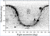 |
Fig. 1 Distribution of the catalogue stars on the sky. The Galactic disk, several star clusters, the Magellanic Clouds, and the Kepler field at [300°,+45°] are visible. |
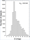 |
Fig. 2 Histogram of the G magnitudes from the Gaia DR2 for 96 549 objects that were successfully cross-matched. The second maximum in the distribution at about G ≈ 16.5 mag is due to stars of the Galactic Bulge. |
3.2 Comparison with the references
We statistically analysed the differences in the reddening values of the individual references among each other and our catalogue. We expect a normal distribution centred at zero with a certain width or standard deviation. Two other important quantities are the third and fourth standardised moments, the skewness and kurtosis (Rice 2006).
The skewness is a measure of symmetry around the zero point or the lack of symmetry. In the ideal case, the skewness for a normal distribution is zero (mean is equal to median), and any symmetric data should have a value near zero. Negative values indicate data that are skewed left in the sense that the left tail of the distribution is long relative to the right one. Values between −0.5 and +0.5 for a large sample, as ours can be considered symmetric. The kurtosis measures whether the data are tailed relative to a normal distribution. The value for an ideal normal distribution is three. Excess kurtosis is often used, subtracting a value of three.
Table 3 presents all statistical values for the different references, whereas Fig. 3 shows the data graphically. The histograms are shown in Figs. A.1–A.4. It has to be kept in mind that these characteristics are for the extinction in (B − V).
All the investigated datasets’ mean and median values are compiled around zero. There are no apparent outliers. The standard deviations for the datasets of the literature vary between 0.12 and 0.23 mag. These values also seem to limit the global statistical accuracy for any of these references. The comparison with our datasets yields slightly higher standard deviations (up to 0.3 mag). We think that the reason is the use of UV data within our compilation. As stated before, it is essential to include this wavelength region, especially for early-type stars (Savage et al. 1985). Looking at the skewness and kurtosis values, we find that only two datasets (Chen et al. 2019; Anders et al. 2022) qualify as being close to normal distributions. All others deviate significantly, especially when it comes to kurtosis. We also calculated all values for those 8500 objects common in all datasets to exclude selection effects. The results are the same, with slightly lower standard deviations.
Figure 3 presents more detailed structures of the individual differences with our catalogue. The asymmetry of the different distributions is visible, especially for the upper main sequence stars (which are, in general, at more considerable distances from the Sun). For the cool-type stars, there is, in four cases, a similar effect in the other direction evident.
In general, we advise the users of the published reddening values to search all available sources and to compare them. The object’s location in the Milky Way needs to be checked for significant deviating values. De-reddening procedures using reddening-free indices, for instance those described in Sec. 2, are always preferable.
Statistical parameters of the differences for the references listed below.
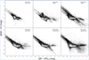 |
Fig. 3 Differences between our reddening estimates and those from the literature, as described in Table 3. We used contours in over-dense regions to clearly show the correlations. |
3.3 Reddening values of open clusters
As the next step, we investigated the members of star clusters in our sample. The releases of the Gaia data brought a flood of newly discovered star clusters based on astrometric and photometric data. However, wrongly identified or already known aggregates make a homogeneous analysis difficult. We used the star cluster membership lists from the catalogue of Hunt & Reffert (2023) to identify possible open cluster members among the studied stars. This catalogue contains the parameters (age, reddening, and distance) of 7167 star clusters, with more than 700 newly discovered high-confidence star clusters. In addition to this, they also include a list of cluster members with membership probabilities for each star. For example, they performed several cross-checks with already published catalogues and found offsets for the extinction (see Fig. 7 therein). We must emphasise that determining the cluster parameters is still challenging, although, from the Gaia datasets, we already get a reasonable estimate of the distances (Netopil et al. 2015; Dias et al. 2021). We cross-matched our sample with the lists by Hunt & Reffert (2023) and identified 4270 high-confidence (P > 0.7) star cluster members. For the comparison, we only took star clusters for which more than two members are included in our sample, leaving us with 786 aggregates. In Fig. 4, we present the comparison result with the published values by Hunt & Reffert (2023). Plotting star clusters with more than five members does not change the results. The skewness and kurtosis of the corresponding distribution are −1.99 and +8.50. We see a wide spread of differences with a clear trend for E(B − V) < 0.2 mag. This means that their Bayesian neural network technique generally overestimates the reddening. This might be a result of the applied binning by Hunt & Reffert (2023) of 0.11 mag in (GBP − GRP). For larger reddening values, the effect reverts. This conclusion is also valid using mean reddening values from the six sources we used for our comparison. Determining the cluster parameters is still very much limited by the choice of reddening. At the same time, the distance can be accurately estimated using the Gaia data (which will improve further with forthcoming releases). We also now have very good metallicities from the Gaia-ESO (Randich et al. 2022) and Galactic Archaeology with Hermes (GALAH, Buder et al. 2021) surveys, for example, which could serve as a starting point for fitting isochrones to get the age. But still, the fitting techniques need to consider all these starting values to derive homogeneous cluster parameters (Pöhnl & Paunzen 2010; Piecka 2021).
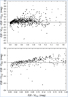 |
Fig. 4 Mean reddening values for members of 786 star clusters from our catalogue (suffix ‘TW’) in comparison with the values from Hunt & Reffert (2023). There is a clear trend for E(B − V) < 0.2 mag. |
3.4 Variable extinction of stellar objects
It has been well documented that several star groups show variable extinction. Most of these objects, like the classical T Tauri and UX Ori stars show this effect because of a varying circumstellar environment (Grankin 2016; Grinin et al. 2019).
On a larger scale, such effects have also been observed for H <sc>II</sc> regions and the Galactic centre (Lebofsky 1979; Vargas Alvarez & Kobulnicky 2013). In general, it can be said that reddening varies in regions with rapid variations in dust and gas content.
Intrinsically variable stars are at the centre of many scientific studies (e.g. Gaia Collaboration 2019). The periods, amplitudes, and light curve characteristics (Sterken & Jaschek 1996) are as manifold as the underlying physical mechanisms (Percy 2007). For example, Cepheid variables and their period-luminosity-relations (Leavitt & Pickering 1912) have allowed us to start constructing a distance ladder, which helped us explore large regions of the Universe. For such studies, the knowledge of a precise extinction value is essential. Therefore, our catalogue can help identify possible outliers and offsets due to incorrect reddening values.
4 Conclusions
Compiling mean reddening values of stellar objects is essential for calibrating and testing observations and models. The interstellar and inter-cluster absorption must be considered for various aspects of astrophysical studies. Its wavelength dependence and different reddening laws due to multiple mixtures of interstellar gas and dust make it necessary to work with a statistically sound sample of objects. We present a catalogue of mean reddening values for 97 826 objects distributed across the visible parts of the Milky Way and the Magellanic Clouds.
A comparison with published reddening values derived via sophisticated automatic fitting procedures reveals systematic offsets for both Galactic field objects and star clusters. Therefore, estimating the reddening using well-established techniques and datasets, especially observations in the UV region, is still essential. Future satellite missions such as the Quick Ultra-VIolet Kilonova surveyor (QUVIK; Werner et al. 2022) will help improve this situation significantly. Also, a (re-)analysis of photometric UV observations available in scientific archives is very much needed (Brown et al. 2014).
Data availability
Full Table 2 is available at the CDS via anonymous ftp to cdsarc.cds.unistra.fr (130.79.128.5) or via https://cdsarc.cds.unistra.fr/viz-bin/cat/J/A+A/689/A270
Acknowledgements
We are grateful to the referee for the constructive input. This work was supported by the grant GAČR 23-07605S and the European Regional Development Fund, project No. ITMS2014+: 313011W085 (MP). This research has made use of the SIMBAD database, operated at CDS, Strasbourg, France and of the Two Micron All Sky Survey (2MASS), which is a joint project of the University of Massachusetts and the Infrared Processing and Analysis Center/California Institute of Technology, funded by the National Aeronautics and Space Administration and the National Science Foundation. This work presents results from the European Space Agency (ESA) space mission Gaia. Gaia data are being processed by the Gaia Data Processing and Analysis Consortium (DPAC). Funding for the DPAC is provided by national institutions, in particular the institutions participating in the Gaia MultiLateral Agreement (MLA). The Gaia mission website is https://www.cosmos.esa.int/gaia. The Gaia archive website is https://archives.esac.esa.int/gaia.
Appendix A Histograms of the reddening differences
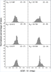 |
Fig. A.1 Histograms of the differences for (1) this work, (2) Chen et al. (2019), (3) Gaia DR2 (Andrae et al. 2018), (4) Gaia DR3 (Gaia Collaboration 2021), (5) StarHorse (Anders et al. 2019), (6) StarHorse2021 (Anders et al. 2022), and (7) Bayestar2019 (Green et al. 2019), as listed in Table 3. |
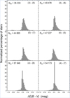 |
Fig. A.2 Histograms of the differences for (1) this work, (2) Chen et al. (2019), (3) Gaia DR2 (Andrae et al. 2018), (4) Gaia DR3 (Gaia Collaboration 2021), (5) StarHorse (Anders et al. 2019), (6) StarHorse2021 (Anders et al. 2022), and (7) Bayestar2019 (Green et al. 2019), as listed in Table 3. |
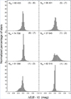 |
Fig. A.3 Histograms of the differences for (1) this work, (2) Chen et al. (2019), (3) Gaia DR2 (Andrae et al. 2018), (4) Gaia DR3 (Gaia Collaboration 2021), (5) StarHorse (Anders et al. 2019), (6) StarHorse2021 (Anders et al. 2022), and (7) Bayestar2019 (Green et al. 2019), as listed in Table 3. |
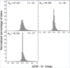 |
Fig. A.4 Histograms of the differences for (1) this work, (2) Chen et al. (2019), (3) Gaia DR2 Andrae et al. (2018), (4) Gaia DR3 (Gaia Collaboration 2021), (5) StarHorse (Anders et al. 2019), (6) StarHorse2021 (Anders et al. 2022), and (7) Bayestar2019 (Green et al. 2019), as listed in Table 3. |
References
- Aidelman, Y., Cidale, L. S., Zorec, J., & Panei, J. A. 2018, A&A, 610, A30 [NASA ADS] [CrossRef] [EDP Sciences] [Google Scholar]
- Alonso-Santiago, J., Marco, A., Negueruela, I., et al. 2018, A&A, 616, A124 [NASA ADS] [CrossRef] [EDP Sciences] [Google Scholar]
- Alonso-Santiago, J., Negueruela, I., Marco, A., et al. 2019, A&A, 631, A124 [NASA ADS] [CrossRef] [EDP Sciences] [Google Scholar]
- Anders, F., Khalatyan, A., Chiappini, C., et al. 2019, A&A, 628, A94 [NASA ADS] [CrossRef] [EDP Sciences] [Google Scholar]
- Anders, F., Khalatyan, A., Queiroz, A. B. A., et al. 2022, A&A, 658, A91 [NASA ADS] [CrossRef] [EDP Sciences] [Google Scholar]
- Andrae, R., Fouesneau, M., Creevey, O., et al. 2018, A&A, 616, A8 [NASA ADS] [CrossRef] [EDP Sciences] [Google Scholar]
- Anthony-Twarog, B. J., & Twarog, B. A. 1994, AJ, 107, 1577 [NASA ADS] [CrossRef] [Google Scholar]
- Bailer-Jones, C. A. L., Rybizki, J., Fouesneau, M., Demleitner, M., & Andrae, R. 2021, AJ, 161, 147 [Google Scholar]
- Barceló Forteza, S., Moya, A., Barrado, D., et al. 2020, A&A, 638, A59 [NASA ADS] [CrossRef] [EDP Sciences] [Google Scholar]
- Belikov, A. N., Kharchenko, N. V., Piskunov, A. E., & Schilbach, E. 1999, A&AS, 134, 525 [NASA ADS] [CrossRef] [EDP Sciences] [Google Scholar]
- Berry, M., Ivezić, Ž., Sesar, B., et al. 2012, ApJ, 757, 166 [Google Scholar]
- Bressan, A., Marigo, P., Girardi, L., et al. 2012, MNRAS, 427, 127 [NASA ADS] [CrossRef] [Google Scholar]
- Brown, P. J., Breeveld, A. A., Holland, S., Kuin, P., & Pritchard, T. 2014, Ap&SS, 354, 89 [Google Scholar]
- Buder, S., Sharma, S., Kos, J., et al. 2021, MNRAS, 506, 150 [NASA ADS] [CrossRef] [Google Scholar]
- Cardelli, J. A., Clayton, G. C., & Mathis, J. S. 1989, ApJ, 345, 245 [Google Scholar]
- Chalov, S. V. 2019, Ap&SS, 364, 175 [NASA ADS] [CrossRef] [Google Scholar]
- Chen, B. Q., Huang, Y., Yuan, H. B., et al. 2019, MNRAS, 483, 4277 [Google Scholar]
- Cochetti, Y. R., Zorec, J., Cidale, L. S., et al. 2020, A&A, 634, A18 [EDP Sciences] [Google Scholar]
- Cortés, C., Maciel, S. C., Vieira, S., et al. 2015, A&A, 581, A68 [NASA ADS] [CrossRef] [EDP Sciences] [Google Scholar]
- Cox, N. L. J., Cami, J., Farhang, A., et al. 2017, A&A, 606, A76 [NASA ADS] [CrossRef] [EDP Sciences] [Google Scholar]
- Cramer, N. 1982, A&A, 112, 330 [NASA ADS] [Google Scholar]
- Cramer, N. 1999, New A Rev., 43, 343 [NASA ADS] [CrossRef] [Google Scholar]
- Creevey, O. L., Sordo, R., Pailler, F., et al. 2023, A&A, 674, A26 [NASA ADS] [CrossRef] [EDP Sciences] [Google Scholar]
- Cummings, J. D., & Kalirai, J. S. 2018, AJ, 156, 165 [Google Scholar]
- Cutri, R. M., Wright, E. L., Conrow, T., Fowler, J. W., Eisenhardt, P. R. M., et al. 2013, VizieR Online Data Catalog: II/328 [Google Scholar]
- Denoyelle, J. 1977, A&AS, 27, 343 [NASA ADS] [Google Scholar]
- Dias, W. S., Monteiro, H., Moitinho, A., et al. 2021, MNRAS, 504, 356 [NASA ADS] [CrossRef] [Google Scholar]
- Domingo, A., & Figueras, F. 1999, A&A, 343, 446 [NASA ADS] [Google Scholar]
- Dougherty, S. M., Waters, L. B. F. M., Burki, G., et al. 1994, A&A, 290, 609 [NASA ADS] [Google Scholar]
- Fitzpatrick, E. L. 1999, PASP, 111, 63 [Google Scholar]
- Gaia Collaboration (Brown, A. G. A., et al.) 2018, A&A, 616, A1 [NASA ADS] [CrossRef] [EDP Sciences] [Google Scholar]
- Gaia Collaboration (Eyer, L., et al.) 2019, A&A, 623, A110 [NASA ADS] [CrossRef] [EDP Sciences] [Google Scholar]
- Gaia Collaboration (Brown, A. G. A., et al.) 2021, A&A, 649, A1 [NASA ADS] [CrossRef] [EDP Sciences] [Google Scholar]
- Garmany, C. D., Glaspey, J. W., Bragança, G. A., et al. 2015, AJ, 150, 41 [CrossRef] [Google Scholar]
- Grankin, K. N. 2016, Astron. Lett., 42, 314 [Google Scholar]
- Gray, R. O., Graham, P. W., & Hoyt, S. R. 2001, AJ, 121, 2159 [NASA ADS] [CrossRef] [Google Scholar]
- Gray, R. O., Riggs, Q. S., Koen, C., et al. 2017, AJ, 154, 31 [NASA ADS] [CrossRef] [Google Scholar]
- Green, G. M., Schlafly, E. F., Finkbeiner, D., et al. 2018, MNRAS, 478, 651 [Google Scholar]
- Green, G. M., Schlafly, E., Zucker, C., Speagle, J. S., & Finkbeiner, D. 2019, ApJ, 887, 93 [NASA ADS] [CrossRef] [Google Scholar]
- Grinin, V. P., Semenov, A. O., Barsunova, O. Y., & Sergeev, S. G. 2019, Astrophysics, 62, 41 [Google Scholar]
- Grosbøl, P. 2016, A&A, 585, A141 [NASA ADS] [CrossRef] [EDP Sciences] [Google Scholar]
- Gutierrez-Moreno, A., & Moreno, H. 1975, PASP, 87, 425 [NASA ADS] [CrossRef] [Google Scholar]
- Hanson, R. J., Bailer-Jones, C. A. L., Burgett, W. S., et al. 2016, MNRAS, 463, 3604 [NASA ADS] [CrossRef] [Google Scholar]
- Hiltner, W. A. 1956, ApJS, 2, 389 [NASA ADS] [CrossRef] [Google Scholar]
- Holmberg, J., Nordström, B., & Andersen, J. 2009, A&A, 501, 941 [NASA ADS] [CrossRef] [EDP Sciences] [Google Scholar]
- Huang, Y., Liu, X. W., Yuan, H. B., et al. 2015, MNRAS, 454, 2863 [NASA ADS] [CrossRef] [Google Scholar]
- Hunt, E. L., & Reffert, S. 2023, A&A, 673, A114 [NASA ADS] [CrossRef] [EDP Sciences] [Google Scholar]
- Hur, H., Park, B.-G., Sung, H., et al. 2015, MNRAS, 446, 3797 [CrossRef] [Google Scholar]
- Johnson, H. L., & Borgman, J. 1963, Bull. Astron. Inst. Netherlands, 17, 115 [NASA ADS] [Google Scholar]
- Kaltcheva, N., & Scorcio, M. 2010, A&A, 514, A59 [NASA ADS] [CrossRef] [EDP Sciences] [Google Scholar]
- Kaltcheva, N. T., Golev, V. K., & Moran, K. 2014, A&A, 562, A69 [NASA ADS] [CrossRef] [EDP Sciences] [Google Scholar]
- Kilkenny, D. 1993, South African Astron. Observ. Circ., 15, 53 [Google Scholar]
- Knapik, A., & Bergeat, J. 1997, A&A, 321, 236 [NASA ADS] [Google Scholar]
- Knapik, A., Bergeat, J., & Rutily, B. 1999, A&A, 344, 263 [NASA ADS] [Google Scholar]
- Kovtyukh, V. V., Soubiran, C., Luck, R. E., et al. 2008, MNRAS, 389, 1336 [NASA ADS] [CrossRef] [Google Scholar]
- Kunder, A., Popowski, P., Cook, K. H., & Chaboyer, B. 2008, AJ, 135, 631 [NASA ADS] [CrossRef] [Google Scholar]
- Kupka, F., & Bruntt, H. 2001, Using TEMPLOGG for Determining Stellar Parameters of MONS Targets, ed. C. Sterken (Brussel: Vrije Universiteit), 39 [Google Scholar]
- Lada, C. J., Lada, E. A., Clemens, D. P., & Bally, J. 1994, ApJ, 429, 694 [NASA ADS] [CrossRef] [Google Scholar]
- Larson, K. A., & Whittet, D. C. B. 2005, ApJ, 623, 897 [NASA ADS] [CrossRef] [Google Scholar]
- Leavitt, H. S., & Pickering, E. C. 1912, Harvard College Observ. Circ., 173, 1 [NASA ADS] [Google Scholar]
- Lebofsky, M. J. 1979, AJ, 84, 324 [NASA ADS] [CrossRef] [Google Scholar]
- Lebzelter, T., Heiter, U., Abia, C., et al. 2012, A&A, 547, A108 [NASA ADS] [CrossRef] [EDP Sciences] [Google Scholar]
- Luck, R. E. 2014, AJ, 147, 137 [Google Scholar]
- Madore, B. F., Freedman, W. L., & Moak, S. 2017, ApJ, 842, 42 [NASA ADS] [CrossRef] [Google Scholar]
- Mahy, L., Rauw, G., De Becker, M., Eenens, P., & Flores, C. A. 2015, A&A, 577, A23 [NASA ADS] [CrossRef] [EDP Sciences] [Google Scholar]
- Majewski, S. R., Schiavon, R. P., Frinchaboy, P. M., et al. 2017, AJ, 154, 94 [NASA ADS] [CrossRef] [Google Scholar]
- Manzo-Martínez, E., Calvet, N., Hernández, J., et al. 2020, ApJ, 893, 56 [CrossRef] [Google Scholar]
- Marco, A., & Negueruela, I. 2013, A&A, 552, A92 [NASA ADS] [CrossRef] [EDP Sciences] [Google Scholar]
- Massey, P., & Johnson, J. 1993, AJ, 105, 980 [Google Scholar]
- Mathis, J. S. 1990, ARA&A, 28, 37 [NASA ADS] [CrossRef] [Google Scholar]
- McCall, B. J., Drosback, M. M., Thorburn, J. A., et al. 2010, ApJ, 708, 1628 [NASA ADS] [CrossRef] [Google Scholar]
- McClure, M. 2009, ApJ, 693, L81 [NASA ADS] [CrossRef] [Google Scholar]
- Megier, A., Krełowski, J., & Weselak, T. 2005, MNRAS, 358, 563 [CrossRef] [Google Scholar]
- Mermilliod, J.-C., Mermilliod, M., & Hauck, B. 1997, A&AS, 124, 349 [NASA ADS] [CrossRef] [EDP Sciences] [Google Scholar]
- Miglio, A., Chiappini, C., Mackereth, J. T., et al. 2021, A&A, 645, A85 [NASA ADS] [CrossRef] [EDP Sciences] [Google Scholar]
- Minniti, D., & Zoccali, M. 2008, IAU Symp., 245, 323 [NASA ADS] [Google Scholar]
- Moitinho, A., Alfaro, E. J., Yun, J. L., & Phelps, R. L. 1997, AJ, 113, 1359 [Google Scholar]
- Napiwotzki, R., Schoenberner, D., & Wenske, V. 1993, A&A, 268, 653 [Google Scholar]
- Neckel, T., & Klare, G. 1980, A&AS, 42, 251 [Google Scholar]
- Neeley, J. R., Marengo, M., Bono, G., et al. 2017, ApJ, 841, 84 [Google Scholar]
- Netopil, M. 2017, MNRAS, 469, 3042 [NASA ADS] [CrossRef] [Google Scholar]
- Netopil, M., Paunzen, E., & Carraro, G. 2015, A&A, 582, A19 [NASA ADS] [CrossRef] [EDP Sciences] [Google Scholar]
- Nieva, M. F., & Przybilla, N. 2012, A&A, 539, A143 [NASA ADS] [CrossRef] [EDP Sciences] [Google Scholar]
- Nikolov, Y. M., Zamanov, R. K., Stoyanov, K. A., & Martí, J. 2017, Bulgarian Astron. J., 27, 10 [Google Scholar]
- Nordström, B., Mayor, M., Andersen, J., et al. 2004, A&A, 418, 989 [Google Scholar]
- Onken, C. A., Wolf, C., Bessell, M. S., et al. 2019, PASA, 36, e033 [Google Scholar]
- Pancino, E., Sanna, N., Altavilla, G., et al. 2021, MNRAS, 503, 3660 [Google Scholar]
- Patriarchi, P., Morbidelli, L., & Perinotto, M. 2003, A&A, 410, 905 [NASA ADS] [CrossRef] [EDP Sciences] [Google Scholar]
- Paunzen, E. 2015, A&A, 580, A23 [NASA ADS] [CrossRef] [EDP Sciences] [Google Scholar]
- Paunzen, E. 2022, A&A, 661, A89 [NASA ADS] [CrossRef] [EDP Sciences] [Google Scholar]
- Paunzen, E., & Netopil, M. 2006, MNRAS, 371, 1641 [NASA ADS] [CrossRef] [Google Scholar]
- Pecaut, M. J., Mamajek, E. E., & Bubar, E. J. 2012, ApJ, 746, 154 [Google Scholar]
- Pejcha, O., & Kochanek, C. S. 2012, ApJ, 748, 107 [Google Scholar]
- Percy, J. R. 2007, Understanding Variable Stars (Cambridge: Cambridge University Press) [CrossRef] [Google Scholar]
- Perry, C. L., & Christodoulou, D. M. 1996, PASP, 108, 772 [NASA ADS] [CrossRef] [Google Scholar]
- Philip, A. G. D., & Egret, D. 1980, A&AS, 40, 199 [NASA ADS] [Google Scholar]
- Piecka, M. 2021, in Star Clusters: the Gaia Revolution. Online workshop, 39 [Google Scholar]
- Pinheiro, M. C., Copetti, M. V. F., & Oliveira, V. A. 2010, A&A, 521, A26 [NASA ADS] [CrossRef] [EDP Sciences] [Google Scholar]
- Pöhnl, H., & Paunzen, E. 2010, A&A, 514, A81 [NASA ADS] [CrossRef] [EDP Sciences] [Google Scholar]
- Queiroz, A. B. A., Anders, F., Santiago, B. X., et al. 2018, MNRAS, 476, 2556 [Google Scholar]
- Raddi, R., Drew, J. E., Fabregat, J., et al. 2013, MNRAS, 430, 2169 [NASA ADS] [CrossRef] [Google Scholar]
- Raddi, R., Drew, J. E., Steeghs, D., et al. 2015, MNRAS, 446, 274 [CrossRef] [Google Scholar]
- Raimond, S., Lallement, R., Vergely, J. L., Babusiaux, C., & Eyer, L. 2012, A&A, 544, A136 [NASA ADS] [CrossRef] [EDP Sciences] [Google Scholar]
- Randich, S., Gilmore, G., Magrini, L., et al. 2022, A&A, 666, A121 [NASA ADS] [CrossRef] [EDP Sciences] [Google Scholar]
- Rebull, L. M., Stauffer, J. R., Cody, A. M., et al. 2018, AJ, 155, 196 [Google Scholar]
- Ren, J. J., Raddi, R., Rebassa-Mansergas, A., et al. 2020, ApJ, 905, 38 [NASA ADS] [CrossRef] [Google Scholar]
- Ren, F., de Grijs, R., Zhang, H., et al. 2021, AJ, 161, 176 [NASA ADS] [CrossRef] [Google Scholar]
- Rice, J. A. 2006, Mathematical Statistics and Data Analysis, 3rd edn. (Belmont, CA: Duxbury Press) [Google Scholar]
- Ripepi, V., Catanzaro, G., Molinaro, R., et al. 2021, MNRAS, 508, 4047 [NASA ADS] [CrossRef] [Google Scholar]
- Sartori, M. J., Lépine, J. R. D., & Dias, W. S. 2003, A&A, 404, 913 [NASA ADS] [CrossRef] [EDP Sciences] [Google Scholar]
- Savage, B. D., Massa, D., Meade, M., & Wesselius, P. R. 1985, ApJS, 59, 397 [Google Scholar]
- Schuster, W. J., & Nissen, P. E. 1989, A&A, 221, 65 [NASA ADS] [Google Scholar]
- Schuster, W. J., Beers, T. C., Michel, R., Nissen, P. E., & García, G. 2004, A&A, 422, 527 [NASA ADS] [CrossRef] [EDP Sciences] [Google Scholar]
- Serkowski, K., Mathewson, D. S., & Ford, V. L. 1975, ApJ, 196, 261 [NASA ADS] [CrossRef] [Google Scholar]
- Skiff, B. A. 2014, VizieR Online Data Catalog: B/mk [Google Scholar]
- Skrutskie, M. F., Cutri, R. M., Stiening, R., et al. 2006, AJ, 131, 1163 [NASA ADS] [CrossRef] [Google Scholar]
- Snow, T. P., J., York, D. G., & Welty, D. E. 1977, AJ, 82, 113 [NASA ADS] [CrossRef] [Google Scholar]
- Sterken, C., & Jaschek, C. 1996, Light Curves of Variable Stars, A Pictorial Atlas (Cambridge: Cambridge University Press) [CrossRef] [Google Scholar]
- Straižys, V., Kazlauskas, A., Boyle, R. P., et al. 2021, AJ, 162, 224 [CrossRef] [Google Scholar]
- Strömgren, B. 1963, QJRAS, 4, 8 [NASA ADS] [Google Scholar]
- Strömgren, B. 1966, ARA&A, 4, 433 [CrossRef] [Google Scholar]
- Swihart, S. J., Garcia, E. V., Stassun, K. G., et al. 2017, AJ, 153, 16 [Google Scholar]
- Terrell, D., Gross, J., & Cooney, W. R. 2012, AJ, 143, 99 [NASA ADS] [CrossRef] [Google Scholar]
- Valencic, L. A., Clayton, G. C., & Gordon, K. D. 2004, ApJ, 616, 912 [NASA ADS] [CrossRef] [Google Scholar]
- Vargas Alvarez, C., & Kobulnicky, H. A. 2013, AAS Meeting Abstracts, 221, 145.07 [NASA ADS] [Google Scholar]
- Vargas Álvarez, C. A., Kobulnicky, H. A., Bradley, D. R., et al. 2013, AJ, 145, 125 [CrossRef] [Google Scholar]
- Voirin, J., Manara, C. F., & Prusti, T. 2018, A&A, 610, A64 [NASA ADS] [CrossRef] [EDP Sciences] [Google Scholar]
- Wang, S., & Chen, X. 2019, ApJ, 877, 116 [Google Scholar]
- Wang, S., Jiang, B. W., Zhao, H., Chen, X., & de Grijs, R. 2017, ApJ, 848, 106 [NASA ADS] [CrossRef] [Google Scholar]
- Werner, N., Řípa, J., Münz, F., et al. 2022, SPIE Conf. Ser., 12181, 121810B [NASA ADS] [Google Scholar]
- Wolf, M. 1923, Astron. Nachr., 219, 109 [NASA ADS] [CrossRef] [Google Scholar]
- Wolff, S. C., Strom, S. E., & Rebull, L. M. 2011, ApJ, 726, 19 [Google Scholar]
- Wright, E. L., Eisenhardt, P. R. M., Mainzer, A. K., et al. 2010, AJ, 140, 1868 [Google Scholar]
- Xiang, M., Rix, H.-W., Ting, Y.-S., et al. 2021, ApJS, 253, 22 [NASA ADS] [CrossRef] [Google Scholar]
- Yanny, B., Rockosi, C., Newberg, H. J., et al. 2009, AJ, 137, 4377 [Google Scholar]
- Zdanavičius, J., & Zdanavičius, K. 2002, Balt. Astron., 11, 441 [NASA ADS] [Google Scholar]
- Zhao, G., Zhao, Y.-H., Chu, Y.-Q., Jing, Y.-P., & Deng, L.-C. 2012, Res. Astron. Astrophys., 12, 723 [NASA ADS] [CrossRef] [Google Scholar]
All Tables
All Figures
|
Fig. 1 Distribution of the catalogue stars on the sky. The Galactic disk, several star clusters, the Magellanic Clouds, and the Kepler field at [300°,+45°] are visible. |
| In the text | |
|
Fig. 2 Histogram of the G magnitudes from the Gaia DR2 for 96 549 objects that were successfully cross-matched. The second maximum in the distribution at about G ≈ 16.5 mag is due to stars of the Galactic Bulge. |
| In the text | |
|
Fig. 3 Differences between our reddening estimates and those from the literature, as described in Table 3. We used contours in over-dense regions to clearly show the correlations. |
| In the text | |
|
Fig. 4 Mean reddening values for members of 786 star clusters from our catalogue (suffix ‘TW’) in comparison with the values from Hunt & Reffert (2023). There is a clear trend for E(B − V) < 0.2 mag. |
| In the text | |
|
Fig. A.1 Histograms of the differences for (1) this work, (2) Chen et al. (2019), (3) Gaia DR2 (Andrae et al. 2018), (4) Gaia DR3 (Gaia Collaboration 2021), (5) StarHorse (Anders et al. 2019), (6) StarHorse2021 (Anders et al. 2022), and (7) Bayestar2019 (Green et al. 2019), as listed in Table 3. |
| In the text | |
|
Fig. A.2 Histograms of the differences for (1) this work, (2) Chen et al. (2019), (3) Gaia DR2 (Andrae et al. 2018), (4) Gaia DR3 (Gaia Collaboration 2021), (5) StarHorse (Anders et al. 2019), (6) StarHorse2021 (Anders et al. 2022), and (7) Bayestar2019 (Green et al. 2019), as listed in Table 3. |
| In the text | |
|
Fig. A.3 Histograms of the differences for (1) this work, (2) Chen et al. (2019), (3) Gaia DR2 (Andrae et al. 2018), (4) Gaia DR3 (Gaia Collaboration 2021), (5) StarHorse (Anders et al. 2019), (6) StarHorse2021 (Anders et al. 2022), and (7) Bayestar2019 (Green et al. 2019), as listed in Table 3. |
| In the text | |
|
Fig. A.4 Histograms of the differences for (1) this work, (2) Chen et al. (2019), (3) Gaia DR2 Andrae et al. (2018), (4) Gaia DR3 (Gaia Collaboration 2021), (5) StarHorse (Anders et al. 2019), (6) StarHorse2021 (Anders et al. 2022), and (7) Bayestar2019 (Green et al. 2019), as listed in Table 3. |
| In the text | |
Current usage metrics show cumulative count of Article Views (full-text article views including HTML views, PDF and ePub downloads, according to the available data) and Abstracts Views on Vision4Press platform.
Data correspond to usage on the plateform after 2015. The current usage metrics is available 48-96 hours after online publication and is updated daily on week days.
Initial download of the metrics may take a while.