| Issue |
A&A
Volume 689, September 2024
|
|
|---|---|---|
| Article Number | A35 | |
| Number of page(s) | 10 | |
| Section | Extragalactic astronomy | |
| DOI | https://doi.org/10.1051/0004-6361/202347593 | |
| Published online | 30 August 2024 | |
Quasi-periodic oscillation analysis for a sample of blazars at the optical band
1
Shandong Provincial Key Laboratory of Optical Astronomy and Solar-Terrestrial Environment, Institute of Space Sciences, Shandong University, Weihai, Shandong 264209, China
2
School of Space Science and Physics, Shandong University, 264209 Weihai, China
Received:
28
July
2023
Accepted:
15
April
2024
Abstract
Context. Quasi-periodic behavior in the light curves of blazars can help us understand the physics. The identification of the supermassive black hole binary (SMBHB) is an active topic, and the periodicity analysis of light curves is a powerful method for searching for these sources.
Aims. In this work, we aim to identify quasi-periodic oscillations (QPOs) in the optical band light curves in our sample and discuss the possible physical origins behind these targets.
Methods. In this study, we collected 155 optical band light curves from three different monitoring programs. We searched for QPOs in our sample using the generalised Lomb-Scargle (GLS) and weighted wavelet Z-transform (WWZ) methods. We simulated 104 artificial light curves and evaluated the significance of the results using the Monte Carlo method.
Results. Our work reveals that 18 targets show QPOs with timescales ranging from 200 days to 1400 days. These QPOs could be explained by three scenarios, including the SMBHB, instability of thick disks and jet precession. Since the frequencies corresponding to QPOs are in the nHz regime, our work provides candidates of SMBHBs for further verification.
Key words: galaxies: active / BL Lacertae objects: general / galaxies: jets / quasars: general
Corresponding author; This email address is being protected from spambots. You need JavaScript enabled to view it. .
© The Authors 2024
 Open Access article, published by EDP Sciences, under the terms of the Creative Commons Attribution License (https://creativecommons.org/licenses/by/4.0), which permits unrestricted use, distribution, and reproduction in any medium, provided the original work is properly cited.
This article is published in open access under the Subscribe to Open model. This email address is being protected from spambots. You need JavaScript enabled to view it. to support open access publication.
1. Introduction
Active galactic nuclei (AGNs) are extreme luminous objects in the sky that have supermassive black holes (SMBHs) in their centers. Blazars from a special subclass of AGNs, whose relativistic jets are oriented toward us (Urry & Padovani 1995). Rapid variability, high polarization and nonthermal emission at all wavelengths are their general observed properties. Blazars are further grouped into the BL Lacertae objects (BL Lacs) and flat-spectrum radio quasars (FSRQs) according to features of emission lines. FSRQs show broad emission lines (equivalent width of >5 Å), whereas BL Lacs show no or narrow emission lines (equivalent width of <5 Å).
The search for the supermassive black hole binary (SMBHB) is an interesting topic in the domain of AGNs. OJ 287 is an established SMBHB; the separation distance of this binary is ∼0.1 pc (Sillanpaa et al. 1988). An et al. (2018) found a SMBHB in the radio galaxy 0402+379 using Very Long Baseline Array (VLBA) observations; this galaxy shows two active nuclei. However, O’Neill et al. (2022) argue that, although the very-long-baseline interferometry (VLBI) method can help us identify the SMBHB, only several nearby targets can be studied due to the restriction of the angular resolution.
Alternatively, Prokhorov & Moraghan (2017) proposed that the quasi-periodic oscillations (QPO) signals of blazars can help us find candidate SMBHBs. Modulated by the binary system, the jets of blazars could produce time series with periodicities (Li et al. 2023). Therefore, we can search for SMBHB candidates by detecting QPOs in the light curves of blazars (Haiman et al. 2009). In addition, O’Neill et al. (2022) proposed that the identification of SMBHBs can provide the properties of gravitational waves and contribute to the development of multimessenger astronomy. Recently, using a pulsar timing data set, Agazie et al. (2023) found the stochastic gravitational-wave (GW) background in the nHz regime. This frequency range is consistent with the GW signal from the SMBHB. Therefore, the study of the QPOs of blazars can play an important role in identifying the SMBHB system.
There is a significant amount of literature on the QPOs of blazars. Those detected in the past few years can be divided into two categories: the long-timescale (several years) QPOs and short-timescale (from days to months) QPOs. The long-timescale QPOs in blazars have been extensively analyzed. Raiteri et al. (2001) studied the periodicity of the BL Lac object AO 0235+16 using the discrete Fourier transform (DFT) and folded light curves, and found a 5.7 yr QPO in the radio band. Bhatta (2017) detected a 270 day QPO along with the harmonics of 550 days and 1150 days in the BL Lac object PKS 0219-164, and offered an explanation for this QPO in that the emission regions move relativistically along the helical path of the magnetized jets. Otero-Santos et al. (2020) found a 3 yr QPO in the BL Lac object 3C 66A, and explained the QPO in terms of the instabilities of the disk. Ren et al. (2021) reported a 4.69 ± 0.14 yr QPO in the BL Lac object PKS J2134-0153. These authors used the SMBHB model to explain this QPO and calculated the distance between the black holes. Gong et al. (2022b) detected a 2.8 yr QPO in the PKS 0405-385, and used the helical motion within the jet and the SMBHB model to explain this QPO behavior. In addition, there are also several works on short-timescale QPOs in blazars. King et al. (2013) found a 120 day QPO in the blazar J1359+4011, and interpreted this QPO as the result of thermal instabilities in the accretion disk. Zhou et al. (2018) detected a 34.5 day QPO in γ-ray light curve of the blazar PKS 2247-131, and explained the QPO as being due to the helical structure of the jet. Gupta et al. (2019) found a 71 day QPO in the blazar B2 1520+31, and explained that this QPO may originate from accretion-disk fluctuations; these authors calculated the mass of the central supermassive black hole, finding ∼5.4 × 10⁹ M⊙. Sarkar et al. (2020) detected a 7.6 day QPO in the blazar CTA 102, and used the helical motion of the enhanced emission in the jet to explain this QPO behavior. Roy et al. (2022) reported two QPOs of the blazar PKS 1510-089 in two different epochs, finding one of a 3.6 days and another of 92 days QPO. These authors explained the 3.6 day QPO in terms of the flux enhancement by magnetic reconnection events and explained the 92 day QPO as the helical motion of a plasma blob in the jet.
The Jurkevich method (Jurkevich 1971), the Lomb-Scargle (LS) periodogram (Lomb 1976; Scargle 1982), structure function (SF) (Simonetti et al. 1985), and REDFIT (Schulz & Mudelsee 2002) are widely used methods to detect QPOs from light curves. However, the maximum value of the LS power is unlimited, which can lead to uncertainties when performing the significance analysis. In addition, these methods can only reveal information in the frequency domain. In the present work, in order to address these issues, we employed the Generalised Lomb-Scargle (GLS) (Zechmeister & Kürster 2009) and the weighted wavelet Z-transform (WWZ) (Foster 1996) methods to detect the QPOs in our sample. The GLS power is generalized, which can minimize uncertainties when performing the significance analysis. The WWZ periodogram can capture information in both the frequency and time domains and reveal how the periodicities change over time. In addition, we used the MC method to evaluate the significance of QPOs.
The fact that QPOs have different timescales may be due to the different mechanisms that produce them. Several possible physical mechanisms have been proposed to explain the long-timescale QPOs: the SMBHB model (Ackermann et al. 2015), jet procession (Romero et al. 2000), and instabilities intrinsic to the accretion disk (Bhatta & Dhital 2020). The short-timescale QPOs can be explained by rotation of the hot spot (Zhang & Bao 1991), the helical jet model (Camenzind & Krockenberger 1992), and the magnetic reconnection model (Huang et al. 2013).
In the last few years, periodicity analyses have mostly dealt with individual sources, and Covino et al. (2018) highlighted the pausity of statistically significant results. Most recently, Ren et al. (2023) searched for QPOs in bright AGN and found that 24 targets show QPOs in their light curves. In the present work, we performed a systematic analysis, searching for potential SMBHB candidates in our sample. The data of the sample in our work cover about 10 years, given that the timescales of the QPOs that can be explained by the SMBHB scenario are measurable in years. We performed the QPO analysis using the GLS and WWZ methods and evaluate their significance using the Monte Carlo method. We also performed a statistical study to find the astrophysical origin of the periodic behavior and to understand the physical mechanisms acting in blazars.
The paper is organized as follows. In Section 2, we describe the data collected during the optical observations. In Section 3, we introduce two common tools in astronomical time-series analyses: the GLS and the WWZ methods. In Section 4, we show how we calculated the GLS power and WWZ power of the sources. In addition, we also present an evaluation of the significance for each target. We then show how we selected the targets with high-significance QPOs (>3σ). Finally, we list the calculation of the targets we selected with QPOs in Table 1. In Section 5, we discuss the model able to explain the QPOs we detected. In addition, we discuss the correlation between the intrinsic period and the redshift of the blazars as well as the correlation between the intrinsic period and masses of supermassive black holes. Finally, we outline our conclusions in Section 6.
Blazars in the sample that show significant QPOs in their fight curves.
2. Sample selection
Many blazar-monitoring programs have provided long-term (more than 10 years) data for blazars suitable for studying the periodicity problem. In this work, we try to systematically search for QPOs in a sample at the optical band.
We collected optical data from three blazar monitoring programs, including the Katzman Automatic Imaging Telescope (KAIT1, 55 000 ≤ MJD ≤ 58 000) (Li et al. 2003), the Small and Moderate Aperture Research Telescope System (SMARTS2, 54 500 ≤ MJD ≤ 57 500) (Bonning et al. 2012), and the Steward observatory (SO3, 55 000 ≤ MJD ≤ 57 900) (Smith et al. 2009). The KAIT has monitored 163 AGNs with an average cadence of 3 days. Li et al. (2003) used two photometry procedures to produce the light curves: PSF-fitting photometry and aperture photometry. The SMARTS monitored all LAT-monitored blazars, and the sampling of the light curves is one point every 2 to 3 days. The SO has monitored gamma-ray-bright blazars and the LAT Monitored Sources using the 2.3 m Bok and 1.54 m Kuiper telescopes.
We selected sources that have been monitored for more than 2500 days and for which at least 150 data points are available, excluding sources that do not satisfy these criteria. Finally, we obtained a sample of 155 targets. Among the sample, 138 targets are monitored by the KAIT, 11 targets are monitored by the SMART, and 6 targets are monitored by the SO. For targets monitored by more than one program, we compared the sampling rate based on the number of data points and the duration of monitoring. For example, the blazar J1256-0547, has been monitored by three programs (KAIT, Smart, and Steward), but we find that KAIT has the best sampling rate, and so we used the KAIT data to perform the periodicity analysis.
3. Periodicity analysis
Fourier transform is a powerful method in time-series analysis; it can be used to transform the signal from the time domain to the frequency domain. The QPO signal in the frequency domain is more evident. In order to detect possible QPOs in the sample we obtained, we used two periodicity analysis methods: the GLS (Zechmeister & Kürster 2009) and the WWZ (Foster 1996). Both irregular sampling and red noise can lead to spurious QPO signals for blazars (Bhatta 2017). The GLS and WWZ methods can reduce the chance probability of producing spurious QPOs caused by irregular sampling. In addition, a significance estimation of the QPO signals can also effectively exclude the spurious signals. In this section, we introduce these two methods and a significance estimation.
3.1. The Generalised Lomb-Scargle
The Lomb-Scargle (LS) periodogram is a common tool used in periodicity analysis; it can be used to effectively analyze unevenly sampled time-series (Lomb 1976, Scargle 1982). However, it has two disadvantages. One is that it does not consider data measurement errors, while the other is that it takes an assumption of the equality between the mean of the data and the mean of the sine function (Zechmeister & Kürster 2009). As opposed to the LS periodogram, the GLS periodogram4 has overcome these two disadvantages, and normalizes the power of the Fourier transform. The GLS power is defined as (Zechmeister & Kürster 2009)
![Mathematical equation: $$ \begin{aligned} P(\omega )=\frac{1}{YY}\left[\frac{{YC_\tau }^2}{CC_\tau }+\frac{{YS_\tau }^2}{SS_\tau }\right], \end{aligned} $$](/articles/aa/full_html/2024/09/aa47593-23/aa47593-23-eq1.gif) (1)
(1)
and
![Mathematical equation: $$ \begin{aligned} YC_\tau&=\sum { w}_i { y}_i C_{i,\tau } -\left[\sum { w}_i { y}_i \right] \left[\sum { w}_i C_{i,\tau }\right], \nonumber \\ YS_\tau&=\sum { w}_i { y}_i S_{i,\tau }-\left[\sum { w}_i { y}_i\right] \left[\sum { w}_i S_{i,\tau }\right],\nonumber \\ CC_\tau&=\sum { w}_i C_{i,\tau }^2-\left[\sum { w}_i C_{i,\tau }\right]^2, \nonumber \\ SS_\tau&=\sum { w}_i S_{i,\tau }^2-\left[\sum { w}_i S_{i,\tau }\right]^2, \nonumber \\ YY&=\sum { w}_i { y}_i^2-\left[\sum { w}_i { y}_i\right]^2, \nonumber \end{aligned} $$](/articles/aa/full_html/2024/09/aa47593-23/aa47593-23-eq2.gif)
where Ci, τ = cos ω(ti − τ) and Si, τ = sin ω(ti − τ), yi is the flux at ti, and σi is the measurement error. The parameter wi is the normalized weight defined as  . The parameter τ is a time reference point defined as
![Mathematical equation: $$ \begin{aligned} \tan 2\omega \tau =\frac{\sum { w}_i\sin 2\omega t_i -2\sum \omega _i\cos \omega t_i\sum { w}_i\sin \omega t_i}{\sum { w}_i\cos 2\omega t_i-[(\sum { w}_i\cos \omega t_i)^2-(\sum { w}_i\sin \omega t_i)^2]}. \end{aligned} $$](/articles/aa/full_html/2024/09/aa47593-23/aa47593-23-eq4.gif) (2)
(2)
We determined the frequency range of the GLS periodogram when performing the GLS method. The frequency range is determined according to the duration of each light curve. For example, the time duration of the KAIT data is 2500 days. We therefore chose a frequency range of [0.0004, 0.01]. In this way, we can reduce the calculation time and exclude some of the spurious signal produced by the red noise. We analyzed all the Optical data in the same way. In the present study, the uncertainties of the periods are the half width at half maximum (HWHMs) of the GLS power peak.
3.2. The weighted wavelet Z-Transform
For comparison, we also used the WWZ5 method to analyze the light curves in our sample. Though the GLS is a useful tool for detecting QPOs in unevenly sampled light curves, it does not solve the problem stemming form the fact that the periodic oscillations for certain targets can change with time (Bhatta 2017). The wavelet analysis, proposed by Torrence & Compo (1998), can fit sine waves in both the time and frequency domains. However, it is not suitable for unevenly sampled time-series. Based on the Morlet wavelet (Grossmann & Morlet 1985), Foster (1996) proposed the WWZ method, which can be used to analyze the unevenly sampled data by means of the vector projection and rescaling the wavelet function. The WWZ map is given by
 (3)
(3)
where  is the effective number, Vx = ∑αwαx2(tα)/∑λwλ − (∑αwαx2(tα)/∑λwλ)2 is the weighted variation of the data, and Vy = ∑αwαy2(tα)/∑λwλ − (∑αwαy2(tα)/∑λwλ)2 is the weighted variation of the model function.
In order to place the QPO signals and their significance in a decipherable manner on the WWZ plot, we normalized the WWZ power in each frequency bin by dividing it by the maximum power across all time bins within each frequency bin. However, O’Neill et al. (2022) normalized the WWZ power by dividing the power by the maximum power of all time bins. After comparison, the time-normalized WWZ can lead to some QPO results appearing more prominently in the time domain, but it increases the relative significance of these QPOs, and causes some false-positive peaks. On the other hand, the frequency-normalized WWZ does not change the relative significance of QPOs in the time domain. Therefore, we chose the frequency-normalized WWZ method to perform periodic analysis in our work.
3.3. Significance estimation
We searched for QPOs in the light curves using the GLS and the WWZ methods. The above two methods are powerful in analyzing the unevenly sampled time series. However, many blazar light curves show the red-noise behavior which may lead to the fake periodic signals (Vaughan et al. 2016). In addition, the uneven sampling of the light curves will also produce false QPOs. Therefore, it is necessary to evaluate the significance of the periodicity signals. We used the MC method to estimate robust significance values for the QPOs in our sample. The MC method is widely adopted to evaluate the significance of certain physical signals.
Our MC recipe includes three steps. First, we model the power spectral density (PSD) and the probability distribution function (PDF) of the observed light curves. We investigate the PSD using the power-law model. Second, based on the model of the PSD and PDFs, we simulate 104 light curves using the Emmanoulopoulos algorithm (Emmanoulopoulos et al. 2013)6, and use the GLS and WWZ methods to analyze these artificial light curves. Each light curve contains the same sampling as the observed light curve to reduce the sampling effect in the significance analysis (Wang & Jiang 2020). Third, we study the distribution of these results and obtain three significance level lines. The 1σ, 2σ, and 3σ significance levels represent probabilities of 68.26%, 95.45%, and 99.73%, respectively. After completing these three steps, we can obtain the significance level for QPO signals.
In order to illustrate the impact of sampling on the results of GLS, we calculated the residuals of the GLS results using the MC method. First, we simulated 104 artificial light curves, which have the same PSD and PDF as the observed light curve. We used the Emmanoulopoulos algorithm to simulate 104 artificial light curves with even samplings, which have the same PSD and PDF as the original light curve. We then calculated the GLS for these evenly sampled light curves. Further, we took the data points with the same sampling as the observed light curve to obtain the unevenly sampled simulated light curve. We calculated the GLS for all these light curves, and obtained their average values. Thus, the residuals can be obtained by subtracting the average GLS of the unevenly sampled sets from that of the evenly sampled sets.
We also plot contour lines on the WWZ map based on the Monte Carlo method, which can be used to estimate the significance of QPOs in the time domain. We simulated 104 artificial light curves, and calculated the WWZ power in each point on the WWZ map. The blue dots in the plot highlight the data points on the WWZ map whose values are greater than 99% of the other points.
4. Analysis and results
To discover QPOs in our large sample within a reasonable timescale, we first carried out the GLS method on each light curve and selected the targets with a maximum GLS power of greater than 0.4. This critical threshold of 0.4 is the result of prior experience with significance estimation for dozens of targets, for that the 3σ significance level in the GLS plot is usually larger than 0.4. In total, we find 35 targets whose maximum GLS power is above this threshold. We then estimated the significance levels using the MC method, and filtered the targets with QPO signals beyond the 3σ significance levels. Finally, we performed the WWZ analysis for these filtered targets in order to further investigate the significance of their QPOs. The significant results of both GLS and WWZ methods are listed in Table 1. In total, we find that 18 targets show QPOs with 3σ significance using both methods, and plot all of them in Figures 1–2.
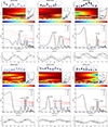 |
Fig. 1. Detection of QPOs in the optical light curves of six blazars of sample. The GLS periodograms are shown in the upper row of each set of panels. The middle row of each set shows the WWZ periodograms. The lower panels show the phase-folded result. |
To the best of our knowledge, we report 13 targets previously undiscovered QPOs, namely J0509+0541, J0630–2406, J0754–1147, J0816–1311, J0820–1258, J0824+5552, J1037+5711, J1243+3627, J1248+5820, J1440+0610, J1642+3948, J1740+5211, and J2055–0021. We also present 7 targets (J0630–2406, J0650+2502, J0754–1147, J0820–1258, J1555+1111, J1740+5211, and J2055–0021) with two QPOs in the GLS periodogram, and 4 targets (J0303–2407, J0509+0541, J0725+1425, and J1440+0610) with three QPOs in the GLS periodogram. We present a detailed analysis of all these targets in the following context.
4.1. GLS periodogram with two peaks
As stated above, there are seven targets that show two peaks in the GLS periodogram. Among them, J0630–2406 and J2055–0021 have one peak with a significance of less than 3σ, and another five targets have two peaks with 3σ significance. It is interesting to find that the ratio of the two periods is typically around 6:5. In the X-ray binaries, Abramowicz & Kluźniak (2001) reported a 3:2 ratio of two QPOs for the target GRO J1655-40, and explained this ratio by the resonance in the system. Strohmayer et al. (2007) found a 4:3 ratio in NGC 5408 X-1, and offered the explanation that these two QPOs belong to different types (type C and B). Bhatta et al. (2023) also reported 22 and 33 day periods in the blazar 3C279, another 3:2 ratio. Therefore, the resonance mechanism may produce the 6:5 ratio in AGN targets. The theoretical derivation of this ratio is still an interesting topic and merits further investigation, but this is beyond the scope of the present work. We also observe that two periods in six targets (including J0630–2406, J0650+2502, J0754–1147, J0820–1258, J1740+5211, J2055–0021) are almost the same, at around 338 and 400 days. Furthermore, the 3σ significance line also shows two weak peaks around these two periods, based on the same sampling but random time series. This leads us to wonder whether or not these two periods could be produced by the uneven sampling of the KAIT program. However, we know of no effective method to exclude the sampling-induced periods.
Although the GLS periodograms of the these targets show two periods, the WWZ periodograms show different results for different targets. We present a description of these targets with two GLS peaks below.
J0630–2406. This target is an FSRQ at z = 1.24. The GLS periodogram shows two distinct peaks centered around 327 days and 421 days. The significance of the QPO at 421 days is over 3σ, whereas the significance of the QPO at 327 days is only 2σ. However, the WWZ periodogram shows two peaks at around 305 days and 760 days. The significance of the QPO at 305 days is over 3σ, while the significance of the QPO at 760 days is lower than 1σ.
J0650+2502. This target is identified as an FSRQ. The GLS periodogram shows two distinct peaks at around 338 days and 404 days, and the significance of both QPOs is over 3σ. Gong et al. (2022a) reported QPOs of 338 days and 406 days in the optical band light curve of this target, which is compatible with our GLS result. In addition, we find a QPO at around 719 days in the WWZ periodogram, which seems to exist throughout the epoch.
J0754–1147. This target is an BL lac. We find two different peaks at 338 days and 411 days in the GLS periodogram with a significance of over 3σ. However, the WWZ periodogram shows two significant QPOs at 270 days and 444 days, respectively. The QPO at 444 days seems to become weaker toward the end of the epoch, the QPO at 270 days seems to develop at the beginning of the observation.
J0820–1258. This target is identified as a BL Lac with a redshift z = 0.54. The GLS periodogram shows two distinct peaks centered around 338 days and 400 days, whose significance is over 3σ. The WWZ periodogram shows three different peaks at around 363 days, 704 days, and 1176 days, respectively. However, the significance of all of these QPOs is lower than 1σ.
J1555+1111. This target is an FSRQ with a redshift of z = 0.36. We find two different peaks in the GLS periodogram at 734 days and 979 days. The significance of both QPOs is over 3σ. However, in the WWZ periodogram, we can find four different peaks centered at around 278 days, 444 days, 1052 days, and 1369 days. The QPOs at 278 days and 444 days seem to occur at the beginning of the observation. Sandrinelli et al. (2018) reported two QPOs at 780 days and 810 days, which are consistent with our results. Ackermann et al. (2015) reported a 2.18 year QPO in γ-ray, radio, and optical band data using the LS method. From our results using WWZ, the QPO at 278 days seems to be most prominent component, and has not been reported before. This may be meaningful for the estimation of the SMBHB. In our work, we calculate the size of a binary system using the same method as Ackermann et al. (2015). Using the period of 278 days, the size of the binary system that forms target J1555+1111 is about 0.002 pc.
J1740+5211. This target is identified as an FSRQ with a redshift of z = 1.38. We detect two QPOs at 344 days and 398 days in the GLS periodogram; the significances of both QPOs are over 3σ. The ratio of these QPOs is consistent with 5:6. It is interesting that we find a more complex structure in the WWZ periodogram of this target. There are four multiple peaks in the WWZ periodogram at 270, 452, 568, and 840 days, respectively. The QPO at 840 days seems to exist from the beginning of the epoch. The QPO at 452 days seems to emerge at around MJD 57500, which is the time when the QPO at 568 days disappears. Alternative QPOs were also found for blazar PKS 2131-021 by (O’Neill et al. 2022). These authors explained this phenomenon by the relative level of activity between the periodic and nonperiodic processes.
J2055–0021. This target is a BL lac. We find two QPOs at 389 days and 337 days in GLS periodogram, and the significance of both QPOs is over 3σ. These two QPOs again conform to the ratio of 6:5. Also, these two QPOs are possibly spurious and due to the specific sampling of KAIT. The WWZ periodogram shows two different QPOs. The QPOs at 325 days and 442 days seem to appear at the beginning of the observation and soon disappear. Both QPOs then emerge at the end of the observation. The results of the WWZ periodogram agree well with the results of the GLS periodogram, although the significance of the results of the WWZ periodogram is less than 1σ.
4.2. GLS periodogram with three peaks
In addition, we find three targets that show three distinct peaks in the GLS periodogram. Here, we provide details of these targets.
J0303–2407. This target is a BL Lac with a redshift of z = 0.27. We find three different peaks at 264, 408, and 899 days in the GLS periodogram. The significance of the QPO at 899 days is over 3σ, while the significance of the QPO at 264 days is over 1σ, and the significance of the QPO at 408 days is over 2σ. In addition, the WWZ periodogram also shows three different peaks centered at around 381, 602, and 952 days. The significance of all the QPOs in the WWZ periodogram is beyond 3σ. The QPOs at 952 days and 381 days seem to exist throughout the observation, while the QPO at 602 days seems to appear at the beginning of the observation and soon disappear. This QPO then emerges at the end of the observation. Interestingly, we find that the QPOs at 408 days and 264 days in the GLS periodogram and the QPOs at 602 days and 381 days in the WWZ periodogram both show a 3:2 ratio. We uses a period of 899 days to phase-fold7 the light curve and obtain two complete cycles.
J0509+0541. The blazar J0509+0541 is a distant FSRQ at z = 0.34. The QPOs of this target are reported for the first time to our knowledge. We find three QPOs in the GLS periodogram, which center at 283, 518, and 1369 days, respectively. The significance of the QPOs at 1369 days and 518 days is over 3σ, whereas the significance of the QPO at 283 days is over 2σ. we also find three distinct peaks at around 444, 806, and 1408 days in the WWZ periodogram. The significance of the QPOs at 444 days and 1408 days is over 3σ, while the significance of the QPO at 806 days is only over 1σ. It is interesting to find that the QPO at 1408 days seems to exist throughout the observation, While the QPO at 444 days seems to gradually grow during the observation.
J0725+1425. This target is identified as an FSRQ with a redshift of z = 1.04. The GLS periodogram shows three different peaks at 284, 539, and 1229 days, respectively. The significance of the QPO at 1229 days is over 3σ, while the significance of the QPO at 539 days is over 2σ, and the significance of the QPO at 284 days is only over 1σ. We also note that the profile of the GLS peaks at 284 days and 539 days is similar to the profile of the significance level lines. Therefore, we consider that these two periods are possibly caused by the uneven sampling of the KAIT program. In addition, we find three different QPOs in the WWZ periodogram, which center at around 304, 581, and 1123 days, respectively. It is interesting to find that the WWZ results are consistent with the GLS results. The significance of the QPO at 304 days is over 3σ, the significance of the QPO at 581 days is less than 1σ, and the significance of the QPO at 1123 days is over 2σ. The QPOs at 1123 days and 304 days seem to exist throughout the observation, while the QPO at 581 days seems to emerge at MJD 57100 and grows stronger toward the end of the epoch. Mi et al. (2020) detected a 0.9±0.15 year QPO for this target using the Jurkevich method to analyze the radio band light curve. Their result is consistent with ours.
J1440+0610. This target is a BL Lac. We detect three distinct peaks at around 278, 534, and 1136 days in the GLS periodogram, respectively. All three peaks have a significance of over 3σ. In addition, this target also shows three distinct peaks at around 287, 507, and 1315 days in the WWZ periodogram, which is consistent with the GLS results. The QPOs at 287 days seems to emerge at the beginning of the observation and becomes weaker until the end of the epoch. The QPOs at 507 days and 1315 days seem to be persistent throughout the observation. Furthermore, we find that the period of 1136 days is double the period of 534 days and quadruple the period of 278 days. Thus, the QPO at 278 (or 287) days seems to be the fundamental, while the QPOs at 534 (or 507) days and 1136 (or 1315) days are harmonics. We also note that there is a 133 day signal in the GLS plot, which is half of the QPO at 278 days, although the significance is only 2σ. However, this QPO of 133 days is not detected in the WWZ periodogram, and therefore its existence remains uncertain.
5. Discussion
In total, we find 18 blazars (including 8 BL Lacs and 10 FSRQs) that show QPOs in their optical light curves. To better understand the origin of these QPOs, we carried out a statistical study of our relatively limited sample, and discuss the possible physical models of QPOs in the following.
5.1. Statistic analysis
In order to study the possible cosmic evolution of the intrinsic periods, we plot the intrinsic period Pint versus the redshift for targets with significant QPO signals. The intrinsic period is defined as
 (4)
(4)
where Pobs is the observed period. For targets with two or three periods, we take the fundamental one as Pobs for the statistical study. As shown in the left panel of Figure 4, there is a weak anti-correlation between the intrinsic period and the redshift. Vestergaard et al. (2008) found that the black hole mass of AGNs is positively correlated with the redshift for AGN objects at z < 2. In the context of the SMBHB scenario, black hole mass is inversely correlated with the orbital periodicity (Fan et al. 2010). Thus, the weak anti-correlation between Pint and z could be explained if the QPOs are indicators of the SMBHB system. However, our sample contains only 15 targets, and may be affected by selection bias.
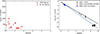 |
Fig. 4. Correlation between the period and the redshift (left panel) as well as the correlation between the period and the supermassive black holes mass (right panel). In the left panel, the red dots represent the FSRQs and red triangles represent the BL Lacs. In the right panel the black dots represent the QPOs in AGNs, the red dots represent the QPOs in intermediate-mass BHs, and the blue dots represent the QPOs in BH X-ray binaries. The gray dash line is given in Abramowicz et al. (2004), the slope of which is −1, while the blue solid line with a slope of −1.27 is the linear fitting result of all points. |
In our sample, we obtain seven targets with information on the mass of their black holes. In the right panel of Figure 4, we plot the intrinsic period versus the mass of the central black hole to find the correlation between them. Abramowicz et al. (2004) proposed that there is an anti-correlation between frequency and black hole mass in high-frequency QPOs, and predicted that AGNs should show the same phenomenon. However, our results suggest that the frequency of AGNs shows a deviation from the prediction of these latter authors. Abramowicz et al. (2004) used the relativistic assumption (the orbital velocity is c) in their work, and obtain a relation whereby the frequency (1/Pint) is inversely related to log M. In the context of AGNs, we can calculate the orbital velocity of the binary black holes via both Kepler’s law and the gravitational radius without the relativistic assumption. We find that the orbital velocity ranges from 0.03 c to 0.06 c. The lower orbital velocity of the binary black holes would produce QPOs at a lower frequency than in the relativistic scenario; this can be used to explain the deviation in the right panel of Figure 4.
5.2. Models
In recent years, several scenarios have been proposed to explain QPOs in blazars, including SMBHBs, instability in the disk-jet system, helical jets, Lense-Thirring precession, and jet precession. These possible explanations are discussed below.
SMBHB: In this scenario, the observed period can be explained by the Keplerian period of the secondary black hole around the primary black hole. The timescale of QPOs caused by SMBHBs ranges from 1 to 25 years (Komossa 2006). This scenario has been widely used to explain the QPOs in several blazars, such as PG 1553+113 (Ackermann et al. 2015), PSO J334.2028+01.4075 (Liu et al. 2015), PKS 0537-441 (Sandrinelli et al. 2016), and S5 0716+714 (Li et al. 2018). The orbit period P can be given by the Kepler’s law, P = 2πa3/2(GM)−1/2, where M is the total mass of the binary system, G is the gravitational constant, and a is the distance between the primary black hole and the secondary black hole. In our work, the timescales of QPOs range from 200 to 1400 days, which is consistent with predictions regarding SMBHBs. Therefore, the SMBHB could be one possible explanation for the QPOs in our sample.
Instability in the disk-jet system: There are two possible explanations in this scenario. Firstly, Bhatta & Dhital (2020) proposed that a bright hotspot on the accretion disk around the central black hole can produce QPOs. Secondly, the instability of the disk can also cause outbursts of the jet, which could produce periodic signals. Zanotti et al. (2003) proposed that oscillations in both thin and thick disks can cause QPOs, but that only the oscillation of the thick disk can cause the long-timescale QPOs with harmonics. In our sample, several sources are indeed accompanied by harmonics, namely J0754-1147, J0820-1258, and J1440+0610. Therefore, this scenario could also account for the year-timescale QPOs in our sample.
Helical jet: The observed QPOs in blazars can be explained by the helical motion of the emission regions in the jets. In this scenario, the periodic change of the viewing angle causes a change in the Doppler factor (δ(t) = 1/Γ(1 − β cos θ(t)), where Γ is the bulk Lorentz factor, β = v/c), which further causes the periodic modulation of the flux. The viewing angle of the emission region can be expressed as θ(t) = sin ϕ sin ψ cos(2πt)+cos ϕ cos ψ, where ϕ is the pitch angle of the helical motion, and ψ is the inclination angle of the jet to the line of sight (Zhou et al. 2018). There are several QPOs in blazars that have been discussed in this model. For example, Conway & Murphy (1993) proposed a helical jet model simulated using three-dimensional magnetohydrodynamics. Roland et al. (1994) reported a quasi-period behavior in 3C 273, and used one component that moves along the helical magnetic field lines to explain this quasi-period behavior. Ostorero et al. (2004) used the helical jet model to explain the QPO of the BL Lac AO 0235+164. Mohan & Mangalam (2015) proposed that a blob in helical motion can cause the jet variability in a general relativistic (GR) model. This model is widely used to explain the short-term transient QPOs in blazars, but cannot provide an appropriate explanation for the year-timescale QPOs in our sample.
Lense-Thirring precession: The QPOs seen in microquasars can be explained by the Lense-Thirring precession of accretion disks, which can produce a thick torus near the central black hole. The precession of this thick torus can change the orientation of the jet in blazars, which can modulate flux periodically. King et al. (2013) used this scenario to explain the QPOs in blazar J1359+4011. This model can be used to explain QPOs acting on short timescales, but Lense-Thirring precession is unlikely to be responsible for long-timescale QPOs. Thus, this scenario is not favored to explain QPOs in this work.
Jet precession: The jet precession can produce the year-timescale QPOs (Liska et al. 2018). Several QPO candidates have been discussed in the context of this scenario. For example, Stirling et al. (2003) reported an approximately two- years periodic oscillating “nozzle” structure in VLBA images of BL Lacertae, and explained this period as being due to periodic variations of the polarization position angle. Caproni et al. (2013) proposed a jet-precession model, which can explain the periodic behavior in the VLBI core of the BL Lac. Therefore, jet precession may be one possible physical mechanism behind the year-timescale QPOs in our sample.
In the particular case of our sample, the timescales of the QPOs range from 200 to 1400 days. As discussed above, such year-timescale QPOs could be caused by SMBHBs, instability in the disk-jet system, or jet precession. Therefore, we prompose that the QPOs detected in our sample could be explained by one of these three scenarios.
6. Conclusions
In the present study, we used the optical data from three optical monitoring programs (KAIT, SMARTS, SO) to detect possible quasi-periodic signals in blazars. This sample enables us to search for and investigate QPOs in blazars, which are meaningful in the multiplemessenger era of astrophysics. Our main results can be summarized as follows.
-
We analyzed the periodicity of the optical light curves for 155 targets. Using the GLS and WWZ methods, we find that 18 blazars (including 8 BL Lacs and 10 FSRQs) showing QPOs with 3σ significance. To the best of our knowledge, this is the first time that QPOs have reported for 13 of these targets. In addition, 7 targets of our sample show two peaks in the GLS periodogram, and 4 targets show three peaks in the GLS periodogram. It is interesting to find that there is a 6:5 period ratio in the targets whose GLS periodogram shows two peaks, these are probably due to a sampling effect of the KAIT program.
-
Our statistical analysis reveals a weak anti-correlation between intrinsic period and redshift, as well as an anti-correlation between intrinsic frequency and black hole mass. We calculated the orbital velocity using Kepler’s law and the gravitational radius, and explain these anti-correlations with the context of the nonrelativistic SMBHB scenario. We propse that the long- timescales of QPOs we find can be explained by either SMBHBs, instability of the thick disk or jet precession. It is worth mentioning that the frequency of the QPOs in our sample is consistent with the nHz frequency of the background gravitational wave. Thus, the blazars in our sample are candidate SMBHBs.
Acknowledgments
This work has been funded by the National Natural Science Foundation of China under grant no. U2031102, and by the Shandong Provincial Natural Science Foundation under grant no. ZR2020MA062. Data from the Steward Observatory spectropolarimetric monitoring project were used. This program is supported by Fermi Guest Investigator grants NNX08AW56G, NNX09AU10G, NNX12AO93G, and NNX15AU81G. This paper has made use of up-to-date SMARTS optical/near-infrared light curves that are available at https://www.astro.yale.edu/smarts/glast/home.php. Our code can be found in https://github.com/Maxwell202117/periodicity/.
References
- Abramowicz, M. A., & Kluźniak, W. 2001, A&A, 374, L19 [NASA ADS] [CrossRef] [EDP Sciences] [Google Scholar]
- Abramowicz, M. A., Kluzniak, W., McClintock, J. E., & Remillard, R. A. 2004, ApJ, 609, L63 [NASA ADS] [CrossRef] [Google Scholar]
- Ackermann, M., Ajello, M., Albert, A., et al. 2015, ApJ, 813, L41 [NASA ADS] [CrossRef] [Google Scholar]
- Agazie, G., Anumarlapudi, A., Archibald, A. M., et al. 2023, ApJ, 951, L8 [NASA ADS] [CrossRef] [Google Scholar]
- An, T., Mohan, P., & Frey, S. 2018, Radio Science, 53, 1211 [NASA ADS] [CrossRef] [Google Scholar]
- Bhatta, G. 2017, ApJ, 847, 7 [NASA ADS] [CrossRef] [Google Scholar]
- Bhatta, G., & Dhital, N. 2020, ApJ, 891, 120 [NASA ADS] [CrossRef] [Google Scholar]
- Bhatta, G., Zola, S., Drozdz, M., et al. 2023, MNRAS, 520, 2633 [NASA ADS] [CrossRef] [Google Scholar]
- Bonning, E., Urry, C. M., Bailyn, C., et al. 2012, ApJ, 756, 13 [Google Scholar]
- Camenzind, M., & Krockenberger, M. 1992, A&A, 255, 59 [NASA ADS] [Google Scholar]
- Caproni, A., Abraham, Z., & Monteiro, H. 2013, MNRAS, 428, 280 [NASA ADS] [CrossRef] [Google Scholar]
- Conway, J. E., & Murphy, D. W. 1993, ApJ, 411, 89 [NASA ADS] [CrossRef] [Google Scholar]
- Covino, S., Sandrinelli, A., & Treves, A. 2018, MNRAS, 482, 1270 [Google Scholar]
- Emmanoulopoulos, D., McHardy, I. M., & Papadakis, I. E. 2013, MNRAS, 433, 907 [NASA ADS] [CrossRef] [Google Scholar]
- Fan, J.-H., Liu, Y., Qian, B.-C., et al. 2010, Res. Astron. Astrophys., 10, 1100 [CrossRef] [Google Scholar]
- Foster, G. 1996, AJ, 112, 1709 [NASA ADS] [CrossRef] [Google Scholar]
- Gong, Y., Yi, T., Yang, X., & Chang, X. 2022a, Astron. Nachr., 343 [CrossRef] [Google Scholar]
- Gong, Y., Zhou, L., Yuan, M., et al. 2022b, ApJ, 931, 168 [CrossRef] [Google Scholar]
- Grossmann, A., & Morlet, J. 1985, Decomposition of Functions into Wavelets of Constant Shape, and Related Transforms (Mathematics + Physics: Lectures on Recent Results), 1 [Google Scholar]
- Gupta, A. C., Tripathi, A., Wiita, P. J., et al. 2019, MNRAS, 484, 5785 [NASA ADS] [Google Scholar]
- Haiman, Z., Kocsis, B., & Menou, K. 2009, ApJ, 700, 1952 [CrossRef] [Google Scholar]
- Huang, C.-Y., Wang, D.-X., Wang, J.-Z., & Wang, Z.-Y. 2013, Res. Astron. Astrophys., 13, 705 [CrossRef] [Google Scholar]
- Jurkevich, I. 1971, Ap&SS, 13, 154 [NASA ADS] [CrossRef] [Google Scholar]
- King, O. G., Hovatta, T., Max-Moerbeck, W., et al. 2013, MNRAS, 436, L114 [NASA ADS] [CrossRef] [Google Scholar]
- Komossa, S. 2006, Mem. Soc. Astron. It., 77, 733 [NASA ADS] [Google Scholar]
- Li, J., Wang, Z., & Zheng, D. 2023, MNRAS, 522, 2928 [NASA ADS] [CrossRef] [Google Scholar]
- Li, W., Filippenko, A. V., Chornock, R., & Jha, S. 2003, PASP, 115, 844 [CrossRef] [Google Scholar]
- Li, X.-P., Luo, Y.-H., Yang, H.-Y., et al. 2018, Ap&SS, 363, 169 [NASA ADS] [CrossRef] [Google Scholar]
- Liska, M., Hesp, C., Tchekhovskoy, A., et al. 2018, MNRAS, 474, L81 [Google Scholar]
- Liu, T., Gezari, S., Heinis, S., et al. 2015, ApJ, 803, L16 [NASA ADS] [CrossRef] [Google Scholar]
- Lomb, N. R. 1976, Astrophys. Space Sci., 39, 447 [Google Scholar]
- Mi, M. I., Xie, Q., Zhong-Zu, W. U., Zhang, L., & Luo, J. J. 2020, Chin. Astron. Astrophys., 44, 313 [Google Scholar]
- Mohan, P., & Mangalam, A. 2015, ApJ, 805, 91 [CrossRef] [Google Scholar]
- O’Neill, S., Kiehlmann, S., Readhead, A. C. S., et al. 2022, ApJ, 926, L35 [CrossRef] [Google Scholar]
- Ostorero, L., Villata, M., & Raiteri, C. M. 2004, A&A, 419, 913 [NASA ADS] [CrossRef] [EDP Sciences] [Google Scholar]
- Otero-Santos, J., Acosta-Pulido, J. A., Becerra González, J., et al. 2020, MNRAS, 492, 5524 [NASA ADS] [CrossRef] [Google Scholar]
- Paliya, V. S., Domínguez, A., Ajello, M., Olmo-García, A., & Hartmann, D. 2021, ApJS, 253, 46 [NASA ADS] [CrossRef] [Google Scholar]
- Prokhorov, D. A., & Moraghan, A. 2017, MNRAS, 471, 3036 [NASA ADS] [CrossRef] [Google Scholar]
- Raiteri, C. M., Villata, M., Aller, H. D., et al. 2001, A&A, 377, 396 [NASA ADS] [CrossRef] [EDP Sciences] [Google Scholar]
- Ren, G.-W., Ding, N., Zhang, X., et al. 2021, MNRAS, 506, 3791 [CrossRef] [Google Scholar]
- Ren, H. X., Cerruti, M., & Sahakyan, N. 2023, A&A, 672, A86 [NASA ADS] [CrossRef] [EDP Sciences] [Google Scholar]
- Roland, J., Teyssier, R., & Roos, N. 1994, A&A, 290, 357 [NASA ADS] [Google Scholar]
- Romero, G. E., Chajet, L., Abraham, Z., & Fan, J. H. 2000, A&A, 360, 57 [NASA ADS] [Google Scholar]
- Roy, A., Sarkar, A., Chatterjee, A., et al. 2022, MNRAS, 510, 3641 [Google Scholar]
- Sandrinelli, A., Covino, S., & Treves, A. 2016, ApJ, 820, 20 [NASA ADS] [CrossRef] [Google Scholar]
- Sandrinelli, A., Covino, S., Treves, A., et al. 2018, A&A, 615, A118 [NASA ADS] [CrossRef] [EDP Sciences] [Google Scholar]
- Sarkar, A., Kushwaha, P., Gupta, A. C., Chitnis, V. R., & Wiita, P. J. 2020, A&A, 642, A129 [NASA ADS] [CrossRef] [EDP Sciences] [Google Scholar]
- Scargle, J. D. 1982, ApJ, 263, 835 [Google Scholar]
- Schulz, M., & Mudelsee, M. 2002, Comput. Geosci., 28, 421 [NASA ADS] [CrossRef] [Google Scholar]
- Sillanpaa, A., Haarala, S., Valtonen, M. J., Sundelius, B., & Byrd, G. G. 1988, ApJ, 325, 628 [NASA ADS] [CrossRef] [Google Scholar]
- Simonetti, J. H., Cordes, J. M., & Heeschen, D. S. 1985, ApJ, 296, 46 [NASA ADS] [CrossRef] [Google Scholar]
- Smith, P. S., Montiel, E., Rightley, S., et al. 2009, Coordinated Fermi/Optical Monitoring of Blazars and the Great 2009 September Gamma-ray Flare of 3C 454.3 [Google Scholar]
- Stirling, A. M., Cawthorne, T. V., Stevens, J. A., et al. 2003, MNRAS, 341, 405 [NASA ADS] [CrossRef] [Google Scholar]
- Strohmayer, T. E., Mushotzky, R. F., Winter, L., et al. 2007, ApJ, 660, 580 [NASA ADS] [CrossRef] [Google Scholar]
- Torrence, C., & Compo, G. P. 1998, Bull. Am. Meteorol. Soc., 79, 61 [Google Scholar]
- Urry, C. M., & Padovani, P. 1995, PASP, 107, 803 [NASA ADS] [CrossRef] [Google Scholar]
- Vaughan, S., Uttley, P., Markowitz, A. G., et al. 2016, MNRAS, 461, 3145 [Google Scholar]
- Vestergaard, M., Fan, X., Tremonti, C. A., Osmer, P. S., & Richards, G. T. 2008, ApJ, 674, L1 [NASA ADS] [CrossRef] [Google Scholar]
- Wang, Y.-F., & Jiang, Y.-G. 2020, ApJ, 902, 41 [NASA ADS] [CrossRef] [Google Scholar]
- Zanotti, O., Rezzolla, L., & Font, J. A. 2003, MNRAS, 341, 832 [NASA ADS] [CrossRef] [Google Scholar]
- Zechmeister, M., & Kürster, M. 2009, A&A, 496, 577 [CrossRef] [EDP Sciences] [Google Scholar]
- Zhang, X. H., & Bao, G. 1991, A&A, 246, 21 [Google Scholar]
- Zhou, J., Wang, Z., Chen, L., et al. 2018, Nat. Commun., 9, 4599 [NASA ADS] [CrossRef] [Google Scholar]
All Tables
All Figures
|
Fig. 1. Detection of QPOs in the optical light curves of six blazars of sample. The GLS periodograms are shown in the upper row of each set of panels. The middle row of each set shows the WWZ periodograms. The lower panels show the phase-folded result. |
| In the text | |
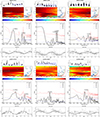 |
Fig. 2. Same as Figure 1, but for six different sources. |
| In the text | |
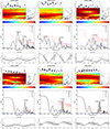 |
Fig. 3. Same as Figure 1, but for another six different sources. |
| In the text | |
|
Fig. 4. Correlation between the period and the redshift (left panel) as well as the correlation between the period and the supermassive black holes mass (right panel). In the left panel, the red dots represent the FSRQs and red triangles represent the BL Lacs. In the right panel the black dots represent the QPOs in AGNs, the red dots represent the QPOs in intermediate-mass BHs, and the blue dots represent the QPOs in BH X-ray binaries. The gray dash line is given in Abramowicz et al. (2004), the slope of which is −1, while the blue solid line with a slope of −1.27 is the linear fitting result of all points. |
| In the text | |
Current usage metrics show cumulative count of Article Views (full-text article views including HTML views, PDF and ePub downloads, according to the available data) and Abstracts Views on Vision4Press platform.
Data correspond to usage on the plateform after 2015. The current usage metrics is available 48-96 hours after online publication and is updated daily on week days.
Initial download of the metrics may take a while.