| Issue |
A&A
Volume 688, August 2024
|
|
|---|---|---|
| Article Number | A207 | |
| Number of page(s) | 13 | |
| Section | Interstellar and circumstellar matter | |
| DOI | https://doi.org/10.1051/0004-6361/202449374 | |
| Published online | 26 August 2024 | |
SRG/eROSITA 3D mapping of the interstellar medium using X-ray absorption spectroscopy
1
Max-Planck-Institut für extraterrestrische Physik,
Gießenbachstraße 1,
85748
Garching,
Germany
e-mail: This email address is being protected from spambots. You need JavaScript enabled to view it.
2
Dr. Karl Remeis-Observatory & ECAP, Friedrich-Alexander-Universität Erlangen-Nürnberg,
Sternwartstr. 7,
96049
Bamberg,
Germany
3
Hamburger Sternwarte, Universität Hamburg,
Gojenbergsweg 112,
21029
Hamburg,
Germany
4
NASA Goddard Space Flight Center,
Greenbelt,
MD
20771,
USA
Received:
29
January
2024
Accepted:
12
June
2024
Abstract
We present a detailed study of the hydrogen density distribution in the local interstellar medium (ISM) using the X-ray absorption technique. Hydrogen column densities were precisely measured by fitting X-ray spectra from coronal sources observed during the initial eROSITA all-sky survey (eRASS1). Accurate distance measurements were obtained through cross-matching Galactic sources with the third Gaia data release (DR3). Despite the absence of a discernible correlation between column densities and distances or Galactic longitude, a robust correlation with Galactic latitude was identified. This suggests a decrease in ISM material density in the vertical direction away from the Galactic plane. We have also investigated the relation between the optical extinction and the hydrogen column density. To do so, we employed multiple density laws to fit the measured column densities, revealing constraints on height scale values (9 < hz < 14 pc). Unfortunately, radial scales and the central density remain unconstrained due to the scarcity of sources near the Galactic center. Subsequently, a 3D density map of the ISM was computed using a Gaussian process approach, inferring hydrogen density distribution from hydrogen column densities. The results unveil the presence of multiple beams and clouds of various sizes, indicative of small-scale structures. High-density regions were identified at approximately 100 pc, consistent with findings in dust-reddening studies, and are potentially associated with the Galactic Perseus arm or the local bubble. Moreover, high-density regions were pinpointed in proximity to the Orion, Chameleon, and Coalsack molecular complex, enriching our understanding of the intricate structure of the local ISM.
Key words: ISM: atoms / ISM: structure / local insterstellar matter / X-rays: ISM
© The Authors 2024
 Open Access article, published by EDP Sciences, under the terms of the Creative Commons Attribution License (https://creativecommons.org/licenses/by/4.0), which permits unrestricted use, distribution, and reproduction in any medium, provided the original work is properly cited.
This article is published in open access under the Subscribe to Open model.
Open Access funding provided by Max Planck Society.
1 Introduction
The interstellar medium (ISM) is one of the most essential constituents of galaxies, affecting the stellar formation and evolutionary processes. This environment includes cold (<104 K), warm (104−106 K), and hot (>106 K) components (see Draine 2011, and references therein). The cold component, in particular, plays a vital role in Galactic evolution given that it is dominated by hydrogen, the most abundant chemical element in the Universe (Sancisi et al. 2008). Multiple radio and Hα surveys have shown that most of the H I gas resides in a thin disk along the Galactic plane, with the Sun embedded within it (Dickey & Lockman 1990; Hartmann & Burton 1997; Bajaja et al. 2005; Kalberla et al. 2005). However, they have limited angular resolution, typically ~0.25 deg2 or larger. 21 cm emission measurements have been used to map the cold component on angular scales of 0.6° in combination with distances inferred from velocities and assuming certain galactic rotation curves (Kalberla et al. 2005; Winkel et al. 2016). However, 21 cm emission measurements cover the entire Galaxy and do not include the molecular component, making it challenging to map local spatial ISM structures.
X-ray absorption measurements constitute a powerful technique to map the ISM in detail. By taking an X-ray source that is acting as a high-energy photon lamp and measuring the absorption spectral features (i.e., spectral edges and absorption lines), one can measure the physical conditions of the ISM. Such analysis enables one to study fine-scale spatial structure and consider the impact of the molecular component, which also affects the shape of the spectra continuum. Moreover, while emission measurements are sensitive to density fluctuations (via the density square dependence on emissivity), the X-ray absorption has a linear dependence of opacity on density. Finally, X-rays generally can probe columns and distances larger than the optical measurements (Gatuzz et al. 2018).
In the last decade, multiple studies have been performed to model the multiphase ISM using high-resolution X-ray spectra (Schulz et al. 2002; Takei et al. 2002; Juett et al. 2004, 2006; Yao et al. 2009; Liao et al. 2013; Pinto et al. 2010, 2013; Gatuzz et al. 2013b,a, 2014, 2015, 2016, 2018, 2021, 2020b; Nicastro et al. 2016a; Gatuzz & Churazov 2018; Eckersall et al. 2017; Psaradaki et al. 2020). Gatuzz et al. (2018), in particular, studied the distribution of the NH in the Milky Way by analyzing X-ray spectra of both Galactic and extragalactic sources. They found a general trend of higher column densities near the Galactic plane for the cold component. They attempted to model the gas distribution with an exponential analytical model. However, the lack of sources near the Galactic plane did not allow them to obtain reasonable constraints for the model parameters.
While it is difficult to disentangle the multiphase ISM using moderate-resolution spectra (although see for counterexample Gatuzz et al. 2020a), CCD spectra allow one to study the equivalent NH absorption of the cold component. Gatuzz et al. (2018) computed a 3D map of the hydrogen density distribution by using the NH measure from XMM-Newton Galactic sources in combination with distances from the first Gaia data release (DR1). They used a Bayesian method explained in Rezaei Kh. et al. (2017) to predict the density distribution even for lines of sight with no initial observations. They found small-scale density structures that analytic density profiles cannot model. However, using Gaia DR1 and needing more flexibility in the modeling led to significant uncertainties in the column densities. Therefore, the maps should be considered qualitatively.
In this paper, we present a 3D map of the hydrogen density distribution in the local ISM obtained from eROSITA spectral fitting in combination with distances obtained from the third Gaia data release (DR3). The all-sky survey conducted by eROSITA offers a unique opportunity for such analysis due to the extensive identification of X-ray Galactic sources. The structure of the present paper is as follows. Section 2 explains the creation of the eROSITA data sample, while Sec. 3 describes the X-ray spectral modeling. Section 4 describes the NH obtained and a comparison with previous results. The modeling of the data with density laws is shown in Sec. 6, while the 3D map computation of the density distribution is described in Sec. 7. Finally, the conclusions are summarized in Sec. 8. For the spectral analysis, we used the xspec data fitting package (version 12.13.11). For the X-ray spectral fits, we assumed χ2 statistics in combination with the Churazov et al. (1996) weighting method, which allows the analysis of data in the low counts regime, providing a goodness-of-fit criterion (see for example, Gatuzz et al. 2019, 2020a). Errors are quoted at a 1σ confidence level unless otherwise stated and abundances are given relative to Grevesse & Sauval (1998). Finally, we denote the column density obtained from X-ray measurements as ![Mathematical equation: $\[N_{\mathrm{H}}^X\]$](/articles/aa/full_html/2024/08/aa49374-24/aa49374-24-eq1.png) .
.
2 eROSITA Galactic objects sample
The eROSITA X-ray telescope (Predehl et al. 2021) on board the Spectrum Rötgen Gamma (SRG) observatory performed the deepest all-sky survey in the soft X-ray energy range (0.2–10 keV). More than 1 million sources were detected by eROSITA during the first all-sky survey (eRASS1), with 80% of the sources being associated with active galactic nuclei (AGNs, Merloni et al. 2024). Freund et al. (2024) performed a cross-matching between the coronal eRASS1 sources and Gaia DR3 (DR3, Gaia Collaboration 2021, 2023) in order to create a catalog of eRASS1 stellar sources, including Gaia distances. By adopting the HamStar identification procedure (Schneider et al. 2022; Freund et al. 2022), they identified 137500 coronal sources with at least one optical counterpart and displayed properties of coronal X-ray sources.
We produced X-ray spectra from this catalog using the eROSITA data analysis software eSASS version 201125 with 010 processing. In particular, we used the srctool task to produce source and background spectra as well as response files for each source identified in Freund et al. (2024). The standard data reduction procedure includes creating circular extraction regions with radii scaled to the maximum likelihood (ML) count rate from the eRASS1 source catalog. Background regions are also created as annuli with sizes scaled to the ML count rate. We combined the data from the telescope modules (TMs) in TM 1–4, 6 and TM 5, 7 because of the excess soft emission due to optical light leaking observed in TM 5 and 7 (Predehl et al. 2021). The last group was analyzed only for energies >1 keV.
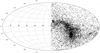 |
Fig. 1 Distribution of the 8231 eRASS1 sources analyzed in this work. |
3 X-ray spectral modeling
Following the work done in Gatuzz et al. (2018), we fit each spectra with multiple models selected to represent in a phenomenological way the most commonly observed spectral shapes in astronomical sources. The models are (using XSPEC nomenclature):
Model A: an absorbed power-law model (XSPEC: tbabs*pow).
Model B: an absorbed thermal model (XSPEC: tbabs*apec).
Model C: an absorbed black-body model (XSPEC: tbabs*bbody).
Model D: an absorbed double thermal model (XSPEC: tbabs*(apec+apec)).
Model E: the same as D but with free abundances for the apec components,
where tbabs is the ISM X-ray absorption model described in Wilms et al. (2000). Then, by fitting the curvature of the X-ray spectra with the models described above, we estimated ![Mathematical equation: $\[N_{\mathrm{H}}^X\]$](/articles/aa/full_html/2024/08/aa49374-24/aa49374-24-eq2.png) values (X for X-rays). The best-fit parameters, the fit-statistic, and statistical uncertainties are available for each model. In the fitting process, we first fixed the hydrogen column density to the value computed by Willingale et al. (2013) and allowed the emission parameters to vary. Then, we kept the
values (X for X-rays). The best-fit parameters, the fit-statistic, and statistical uncertainties are available for each model. In the fitting process, we first fixed the hydrogen column density to the value computed by Willingale et al. (2013) and allowed the emission parameters to vary. Then, we kept the ![Mathematical equation: $\[N_{\mathrm{H}}^X\]$](/articles/aa/full_html/2024/08/aa49374-24/aa49374-24-eq3.png) as a free parameter and proceeded to compute the uncertainties. After all models were applied, the final
as a free parameter and proceeded to compute the uncertainties. After all models were applied, the final ![Mathematical equation: $\[N_{\mathrm{H}}^X\]$](/articles/aa/full_html/2024/08/aa49374-24/aa49374-24-eq4.png) value for our analysis was selected from the model for which chisqr/d.o.f. is close to 1.0. It is important to note that in this study, our main interest is to obtain the most accurate emission+absorption fit to measure
value for our analysis was selected from the model for which chisqr/d.o.f. is close to 1.0. It is important to note that in this study, our main interest is to obtain the most accurate emission+absorption fit to measure ![Mathematical equation: $\[N_{\mathrm{H}}^X\]$](/articles/aa/full_html/2024/08/aa49374-24/aa49374-24-eq5.png) instead of the physical conditions of the Galactic sources.
instead of the physical conditions of the Galactic sources.
We obtained constrained column densities for 8231 eRASS1 sources, a sample almost one order of magnitude larger than the analysis done by Gatuzz et al. (2018). We obtained only upper limits or unrealistic values (e.g., <1015 cm−2) for the rest of the sources, due to the poor statistics in the spectra. We notice that in most cases, the best statistical fit was obtained for models D-E (~80%), which points out the complexity of the coronal spectra modeling (see for example Robrade et al. 2012; Coffaro et al. 2022). Figure 1 shows the distribution of the sources in the Aitoff projection. Due to the SRG scanning strategy, sources near the ecliptic equator are observed six times during one day, while sources at higher ecliptic latitudes are observed for longer periods of time (>10 ks). It is worth noting that the German eROSITA consortium only has access to the western hemisphere. The top panel of Fig. 2 shows the distribution of the sources as a function of the number of counts in the 0.2–10 keV energy range. As an X-ray survey, the snapshot observations lead to many sources being in the low-count regime. The bottom panel of Fig. 2 shows the distribution of the sources as a function of the Gaia distances (r). A normal distribution can be distinguished, with a peak around 125 pc, although distances >1000 pc are also covered. Such a distribution indicates that our analysis of the ![Mathematical equation: $\[N_{\mathrm{H}}^X\]$](/articles/aa/full_html/2024/08/aa49374-24/aa49374-24-eq6.png) distribution corresponds to the local ISM.
distribution corresponds to the local ISM.
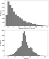 |
Fig. 2 Distribution of sources as a function of different parameters. Top panel: distribution of sources as a function of the number of counts in the 0.2–10 keV energy range. Bottom panel: distribution of sources as a function of the distance obtained from the Gaia observatory. |
4 Hydrogen column densities
Figure 3 shows an Aitoff projection of the Galactic sources analyzed for different distance ranges. The log(![Mathematical equation: $\[N_{\mathrm{H}}^X\]$](/articles/aa/full_html/2024/08/aa49374-24/aa49374-24-eq7.png) ) values obtained from the X-ray spectral fitting procedure described above are indicated by colors in units of cm−2. Although most sources are concentrated near the Galactic plane, the sample includes many high-latitude sources. We have found an average column density of
) values obtained from the X-ray spectral fitting procedure described above are indicated by colors in units of cm−2. Although most sources are concentrated near the Galactic plane, the sample includes many high-latitude sources. We have found an average column density of ![Mathematical equation: $\[N_{\mathrm{H}}^X=(0.15 \pm 0.05) \times 10^{22} \mathrm{~cm}^{-2}\]$](/articles/aa/full_html/2024/08/aa49374-24/aa49374-24-eq8.png) .
.
Figure 4 shows the ![Mathematical equation: $\[N_{\mathrm{H}}^X\]$](/articles/aa/full_html/2024/08/aa49374-24/aa49374-24-eq9.png) distribution as a function of the number of counts in the 0.2–10 keV energy range. We note that five objects have a number of counts > log(3.2). However, we zoomed in on the plot for clarity. We applied a rebinning procedure to our dataset to facilitate visualization, while preserving essential features. Specifically, we grouped the original dataset into larger bins, each encompassing approximately 200 data points, with error bars indicating the uncertainties of the sample of sources within each bin. This rebinning process was executed to mitigate visual clutter and emphasize overarching trends in the data, allowing for clearer interpretation. While this approach sacrifices some fine-scale resolution, it enables a more coherent depiction of the dataset’s overall characteristics and analysis. We note that for this sample a broad range of
distribution as a function of the number of counts in the 0.2–10 keV energy range. We note that five objects have a number of counts > log(3.2). However, we zoomed in on the plot for clarity. We applied a rebinning procedure to our dataset to facilitate visualization, while preserving essential features. Specifically, we grouped the original dataset into larger bins, each encompassing approximately 200 data points, with error bars indicating the uncertainties of the sample of sources within each bin. This rebinning process was executed to mitigate visual clutter and emphasize overarching trends in the data, allowing for clearer interpretation. While this approach sacrifices some fine-scale resolution, it enables a more coherent depiction of the dataset’s overall characteristics and analysis. We note that for this sample a broad range of ![Mathematical equation: $\[N_{\mathrm{H}}^X\]$](/articles/aa/full_html/2024/08/aa49374-24/aa49374-24-eq10.png) measurements can be obtained, and we have been able to recover low column densities (< 1021 cm−2). We found that the average uncertainty for the sample is 35%, which decreases to 15% for sources with > log(2.5) number of counts.
measurements can be obtained, and we have been able to recover low column densities (< 1021 cm−2). We found that the average uncertainty for the sample is 35%, which decreases to 15% for sources with > log(2.5) number of counts.
Figure 5 shows the ![Mathematical equation: $\[N_{\mathrm{H}}^X\]$](/articles/aa/full_html/2024/08/aa49374-24/aa49374-24-eq11.png) distribution as a function of the distance for each source. The data has been rebinned for illustrative purposes. The hydrogen column densities range from 1019 to 1022 cm−2. There is no clear correlation between the column densities and the distances, which was expected, given that not only the distances but also the position of the source (i.e., the celestial coordinates) affects the density of the absorber.
distribution as a function of the distance for each source. The data has been rebinned for illustrative purposes. The hydrogen column densities range from 1019 to 1022 cm−2. There is no clear correlation between the column densities and the distances, which was expected, given that not only the distances but also the position of the source (i.e., the celestial coordinates) affects the density of the absorber.
Figure 6 shows the column densities’ distribution as a function of the Galactic latitude (top panel) and Galactic longitude (bottom panel). We found a solid correlation of the ![Mathematical equation: $\[N_{\mathrm{H}}^X\]$](/articles/aa/full_html/2024/08/aa49374-24/aa49374-24-eq12.png) values with the Galactic latitude, which indicates a decrease in the ISM material density in the vertical direction away from the Galactic plane. Establishing a clear relationship between
values with the Galactic latitude, which indicates a decrease in the ISM material density in the vertical direction away from the Galactic plane. Establishing a clear relationship between ![Mathematical equation: $\[N_{\mathrm{H}}^X\]$](/articles/aa/full_html/2024/08/aa49374-24/aa49374-24-eq13.png) and the Galactic longitude is difficult. As was indicated before, the rebinning of the data led to a loss of fine-scale structures.
and the Galactic longitude is difficult. As was indicated before, the rebinning of the data led to a loss of fine-scale structures.
4.1 Comparison with previous X-ray interstellar medium absorption analysis
We have measured a range of column densities for the cold component in good agreement with previous high-resolution spectra analysis (see, for example Pinto et al. 2013; Gatuzz et al. 2016, 2018; Eckersall et al. 2017). Gatuzz et al. (2018), in particular, found a similar correlation between ![Mathematical equation: $\[N_{\mathrm{H}}^X\]$](/articles/aa/full_html/2024/08/aa49374-24/aa49374-24-eq14.png) values and the Galactic latitude and longitude from a sample including both Galactic and extragalactic sources. However, most works based on high-resolution spectra have used X-ray binaries (XBs) as Galactic sources, and have thus avoided studying regions close to the Galactic plane. Gatuzz et al. (2018) also observe a general trend of higher column densities near the Galactic plane in their analysis. A primary difference between our results and their measurements is that we can recover low column densities (< 1020 cm−2) for Galactic latitudes (i.e., |b| > 20°). This is most likely model-related, as Gatuzz et al. (2018) only considered single-temperature coronal models, and they fixed the abundance of the Galactic X-ray sources to solar values.
values and the Galactic latitude and longitude from a sample including both Galactic and extragalactic sources. However, most works based on high-resolution spectra have used X-ray binaries (XBs) as Galactic sources, and have thus avoided studying regions close to the Galactic plane. Gatuzz et al. (2018) also observe a general trend of higher column densities near the Galactic plane in their analysis. A primary difference between our results and their measurements is that we can recover low column densities (< 1020 cm−2) for Galactic latitudes (i.e., |b| > 20°). This is most likely model-related, as Gatuzz et al. (2018) only considered single-temperature coronal models, and they fixed the abundance of the Galactic X-ray sources to solar values.
4.2 Comparison with 21 cm surveys
The top panel in Fig. 7 shows a comparison between the ![Mathematical equation: $\[N_{\mathrm{H}}^X\]$](/articles/aa/full_html/2024/08/aa49374-24/aa49374-24-eq15.png) and the
and the ![Mathematical equation: $\[N_{\mathrm{H}}^{21 \mathrm{cm}}\]$](/articles/aa/full_html/2024/08/aa49374-24/aa49374-24-eq16.png) measured in the lines of sight. The data has been rebinned for illustrative purposes. We obtained the values from Willingale et al. (2013), which include not only the atomic component but also the molecular component (H2). While estimating the expected
measured in the lines of sight. The data has been rebinned for illustrative purposes. We obtained the values from Willingale et al. (2013), which include not only the atomic component but also the molecular component (H2). While estimating the expected ![Mathematical equation: $\[N_{\mathrm{H}_2}\]$](/articles/aa/full_html/2024/08/aa49374-24/aa49374-24-eq17.png) for any particular direction is difficult, Willingale et al. (2013) derived an empirical function dependent on the product of the atomic hydrogen column densities from Kalberla et al. (2005) and dust extinction measurements from Schlegel et al. (1998). Such values constitute a revision of previous standard methods, particularly at low Galactic latitudes. They estimated systematic uncertainty values of ~16% for column densities lower than ~1.5 × 1021cm-2. Such uncertainties will impact the correlation between
for any particular direction is difficult, Willingale et al. (2013) derived an empirical function dependent on the product of the atomic hydrogen column densities from Kalberla et al. (2005) and dust extinction measurements from Schlegel et al. (1998). Such values constitute a revision of previous standard methods, particularly at low Galactic latitudes. They estimated systematic uncertainty values of ~16% for column densities lower than ~1.5 × 1021cm-2. Such uncertainties will impact the correlation between ![Mathematical equation: $\[N_{\mathrm{H}}^X\]$](/articles/aa/full_html/2024/08/aa49374-24/aa49374-24-eq18.png) and
and ![Mathematical equation: $\[N_{\mathrm{H}}^{21 \mathrm{cm}}\]$](/articles/aa/full_html/2024/08/aa49374-24/aa49374-24-eq19.png) measurements.
measurements.
In general, the values are better distributed around the log(![Mathematical equation: $\[N_{\mathrm{H}}^X\]$](/articles/aa/full_html/2024/08/aa49374-24/aa49374-24-eq22.png) )/log(
)/log(![Mathematical equation: $\[N_{\mathrm{H}}^{21 \mathrm{cm}}\]$](/articles/aa/full_html/2024/08/aa49374-24/aa49374-24-eq23.png) ) unity ratio than Gatuzz et al. (2018, see their Fig. 6). However, there are high-density points where
) unity ratio than Gatuzz et al. (2018, see their Fig. 6). However, there are high-density points where ![Mathematical equation: $\[N_{\mathrm{H}}^X\]$](/articles/aa/full_html/2024/08/aa49374-24/aa49374-24-eq24.png) values tend to be lower than
values tend to be lower than ![Mathematical equation: $\[N_{\mathrm{H}}^{21 \mathrm{cm}}\]$](/articles/aa/full_html/2024/08/aa49374-24/aa49374-24-eq25.png) . The log(
. The log(![Mathematical equation: $\[N_{\mathrm{H}}^X\]$](/articles/aa/full_html/2024/08/aa49374-24/aa49374-24-eq26.png) )/log(
)/log(![Mathematical equation: $\[N_{\mathrm{H}}^{21 \mathrm{cm}}\]$](/articles/aa/full_html/2024/08/aa49374-24/aa49374-24-eq27.png) ) = 1 ratio is plotted with a solid blue line. The bottom panel in Fig. 7 shows a comparison between the
) = 1 ratio is plotted with a solid blue line. The bottom panel in Fig. 7 shows a comparison between the ![Mathematical equation: $\[N_{\mathrm{H}}^X\]$](/articles/aa/full_html/2024/08/aa49374-24/aa49374-24-eq28.png) and the
and the ![Mathematical equation: $\[N_{\mathrm{H}}^{21 \mathrm{cm}}\]$](/articles/aa/full_html/2024/08/aa49374-24/aa49374-24-eq29.png) measured in the lines of sight but including only high-latitude (|b| > 75°) and low-latitude (|b| < 15°) sources. It is clear that the disagreement with the
measured in the lines of sight but including only high-latitude (|b| > 75°) and low-latitude (|b| < 15°) sources. It is clear that the disagreement with the ![Mathematical equation: $\[N_{\mathrm{H}}^{21 \mathrm{cm}}+N_{\mathrm{H}_2}\]$](/articles/aa/full_html/2024/08/aa49374-24/aa49374-24-eq30.png) values is larger for low-latitude sources, as was expected, given the increase in the H2 contribution as we move toward the Galactic plane.
values is larger for low-latitude sources, as was expected, given the increase in the H2 contribution as we move toward the Galactic plane.
As was described above, our ![Mathematical equation: $\[N_{\mathrm{H}}^X\]$](/articles/aa/full_html/2024/08/aa49374-24/aa49374-24-eq35.png) measurements allowed us to recover low column densities. Also, 21 cm maps provide measurements over the entire Galactic line of sight. Therefore, they can lead to overestimating the column densities for near sources. Analysis done with high-resolution spectra tends to show lower X-ray column densities than 21 cm measurements (see for example Gatuzz & Churazov 2018). Lines of sight in which
measurements allowed us to recover low column densities. Also, 21 cm maps provide measurements over the entire Galactic line of sight. Therefore, they can lead to overestimating the column densities for near sources. Analysis done with high-resolution spectra tends to show lower X-ray column densities than 21 cm measurements (see for example Gatuzz & Churazov 2018). Lines of sight in which ![Mathematical equation: $\[N_{\mathrm{H}}^X\]$](/articles/aa/full_html/2024/08/aa49374-24/aa49374-24-eq36.png) is larger than 21 cm measurements may correspond to regions with absorbers other than atomic hydrogen, including partially ionized gas (e.g., Gatuzz et al. 2016) or molecular absorption (Joachimi et al. 2016), a scenario proposed by Willingale et al. (2013). Finally, differences between 21 cm and X-ray values may be related to the difference in effective beam sizes. While the size of regions probed by X-ray measurements is limited by the size of the distant source, 21 cm measurements come from a beam size of ~0.7 deg2 (Kalberla et al. 2005).
is larger than 21 cm measurements may correspond to regions with absorbers other than atomic hydrogen, including partially ionized gas (e.g., Gatuzz et al. 2016) or molecular absorption (Joachimi et al. 2016), a scenario proposed by Willingale et al. (2013). Finally, differences between 21 cm and X-ray values may be related to the difference in effective beam sizes. While the size of regions probed by X-ray measurements is limited by the size of the distant source, 21 cm measurements come from a beam size of ~0.7 deg2 (Kalberla et al. 2005).
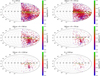 |
Fig. 3 Distribution of the sources for different distance ranges in Aitoff projection. The colors indicate the log( |
![Mathematical equation: $\[N_{\mathrm{H}}^X\]$](/articles/aa/full_html/2024/08/aa49374-24/aa49374-24-eq20.png)
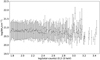 |
Fig. 4
|
![Mathematical equation: $\[N_{\mathrm{H}}^X\]$](/articles/aa/full_html/2024/08/aa49374-24/aa49374-24-eq21.png)
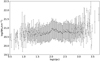 |
Fig. 5
|
![Mathematical equation: $\[N_{\mathrm{H}}^X\]$](/articles/aa/full_html/2024/08/aa49374-24/aa49374-24-eq31.png)
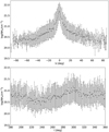 |
Fig. 6
|
![Mathematical equation: $\[N_{\mathrm{H}}^X\]$](/articles/aa/full_html/2024/08/aa49374-24/aa49374-24-eq32.png)
![Mathematical equation: $\[N_{\mathrm{H}}^X\]$](/articles/aa/full_html/2024/08/aa49374-24/aa49374-24-eq33.png)
![Mathematical equation: $\[N_{\mathrm{H}}^X\]$](/articles/aa/full_html/2024/08/aa49374-24/aa49374-24-eq34.png)
5 The gas-to-extinction ratio
Figure 8 compares ![Mathematical equation: $\[N_{\mathrm{H}}^X\]$](/articles/aa/full_html/2024/08/aa49374-24/aa49374-24-eq37.png) as a function of the extinction in the lines of sight. Black data points correspond to the
as a function of the extinction in the lines of sight. Black data points correspond to the ![Mathematical equation: $\[N_{\mathrm{H}}^X\]$](/articles/aa/full_html/2024/08/aa49374-24/aa49374-24-eq38.png) values obtained from the best fit. Extinction values were computed from Schlafly & Finkbeiner (2011) with the SDSS red filter (6231 Å). In particular, we used the dustmap python package2 to compute extinction maps developed by Green (2018). Regarding the uncertainties on the extinction calculation, Schlafly & Finkbeiner (2011) indicate that ΔAV < 56 × 10−3 mag. Similar to Zhu et al. (2017, see their Eq. (3)), we computed a linear fit to the data in the form
values obtained from the best fit. Extinction values were computed from Schlafly & Finkbeiner (2011) with the SDSS red filter (6231 Å). In particular, we used the dustmap python package2 to compute extinction maps developed by Green (2018). Regarding the uncertainties on the extinction calculation, Schlafly & Finkbeiner (2011) indicate that ΔAV < 56 × 10−3 mag. Similar to Zhu et al. (2017, see their Eq. (3)), we computed a linear fit to the data in the form
![Mathematical equation: $\[N_{\mathrm{H}}^X=MA_{\mathrm{V}}(\mathrm{mag})+B.\]$](/articles/aa/full_html/2024/08/aa49374-24/aa49374-24-eq39.png) (1)
(1)
The best-fit parameters are M = (4.82 ± 0.08) × 1021 cm−2 mag−1 and B = (0.59 ± 0.16) ×1021 cm−2, and the solid blue line in the plot shows the best-fit result. The zero-point offset value may indicate the effects of a molecular hydrogen contribution as its value is larger than those column densities found for large latitudes (see bottom panel in Fig. 7). Our linear fit appears to underestimate the data quite strongly at larger AV. Some potential reasons include variability in dust properties (due to composition, size distribution etc.) across different lines of sight, nonlinear effects or variations due to the complex interplay between gas and dust phases, and physical processes such as clumpiness or variations in metallicity.
The slope found from the best fit is larger than the value obtained in previous studies by Zhu et al. (2017, (M = 2.25 ± 0.03) ×1021), Foight et al. (2016, (M = 2.87 ± 0.12) × 1021), Valencic & Smith (2015, (M = 2.08 ± 0.30) × 1021), Watson (2011, ![Mathematical equation: $\[\left.\left(M=2.20_{-0.40}^{+0.30}\right) \times 10^{21}\right)\]$](/articles/aa/full_html/2024/08/aa49374-24/aa49374-24-eq48.png) , Güver & Özel (2009, (M = 2.21 ± 0.09) ×1021), and Predehl & Schmitt (1995, (M = 1.79 ± 0.03) × 1021). In this regard, it is important to note that these studies (i) are based on a much smaller sample of <30 sources, except for Watson (2011, ~100 sources); (ii) include supernova remnants (SNRs), XBs, and planetary nebulae (PNe), and thus intrinsic absorption may affect their measurement; (iii) while they include large distances (up to ~13 kpc), most of the sources cover Galactic latitude ranges of |b|<30°, limiting their analysis to the Galactic plane; (iv) assume different interstellar abundance standards.
, Güver & Özel (2009, (M = 2.21 ± 0.09) ×1021), and Predehl & Schmitt (1995, (M = 1.79 ± 0.03) × 1021). In this regard, it is important to note that these studies (i) are based on a much smaller sample of <30 sources, except for Watson (2011, ~100 sources); (ii) include supernova remnants (SNRs), XBs, and planetary nebulae (PNe), and thus intrinsic absorption may affect their measurement; (iii) while they include large distances (up to ~13 kpc), most of the sources cover Galactic latitude ranges of |b|<30°, limiting their analysis to the Galactic plane; (iv) assume different interstellar abundance standards.
Figure 9 shows the distribution of the ![Mathematical equation: $\[N_{\mathrm{H}}^X / A_{\mathrm{V}}\]$](/articles/aa/full_html/2024/08/aa49374-24/aa49374-24-eq49.png) ratio as a function of the Galactic longitude (top panel) and Galactic latitude (bottom panel) in the lines of sight. While there is no clear indication of variations along the Galactic longitude, the
ratio as a function of the Galactic longitude (top panel) and Galactic latitude (bottom panel) in the lines of sight. While there is no clear indication of variations along the Galactic longitude, the ![Mathematical equation: $\[N_{\mathrm{H}}^X / A_{\mathrm{V}}\]$](/articles/aa/full_html/2024/08/aa49374-24/aa49374-24-eq50.png) value decreases as we move toward the Galactic plane. From 928 sources located at Galactic latitude |b| < 5° in our sample, we found 757 sources for which the
value decreases as we move toward the Galactic plane. From 928 sources located at Galactic latitude |b| < 5° in our sample, we found 757 sources for which the ![Mathematical equation: $\[N_{\mathrm{H}}^X / A_{\mathrm{V}}\]$](/articles/aa/full_html/2024/08/aa49374-24/aa49374-24-eq51.png) is lower than 1.0. This may reflect the increase in the dust ISM component toward the Galactic plane. (Dame et al. 2001; Weingartner & Draine 2001; Green et al. 2018).
is lower than 1.0. This may reflect the increase in the dust ISM component toward the Galactic plane. (Dame et al. 2001; Weingartner & Draine 2001; Green et al. 2018).
Figure 10 shows the ![Mathematical equation: $\[N_{\mathrm{H}}^X / A_{\mathrm{V}}\]$](/articles/aa/full_html/2024/08/aa49374-24/aa49374-24-eq52.png) ratio as a function of (a) the distance from the Galactic center, assuming that Rsun = 8.5 kpc (Rg); (b) the distance from the Galactic plane (z), and (c)
ratio as a function of (a) the distance from the Galactic center, assuming that Rsun = 8.5 kpc (Rg); (b) the distance from the Galactic plane (z), and (c) ![Mathematical equation: $\[N_{\mathrm{H}}^X\]$](/articles/aa/full_html/2024/08/aa49374-24/aa49374-24-eq53.png) . There is a hint of increasing
. There is a hint of increasing ![Mathematical equation: $\[N_{\mathrm{H}}^X / A_{\mathrm{V}}\]$](/articles/aa/full_html/2024/08/aa49374-24/aa49374-24-eq54.png) as a function of z and
as a function of z and ![Mathematical equation: $\[N_{\mathrm{H}}^X\]$](/articles/aa/full_html/2024/08/aa49374-24/aa49374-24-eq55.png) . However, the uncertainties are significant.
. However, the uncertainties are significant.
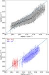 |
Fig. 7 Comparison between |
![Mathematical equation: $\[N_{\mathrm{H}}^X\]$](/articles/aa/full_html/2024/08/aa49374-24/aa49374-24-eq40.png)
![Mathematical equation: $\[N_{\mathrm{H}}^{21 \mathrm{cm}}\]$](/articles/aa/full_html/2024/08/aa49374-24/aa49374-24-eq41.png)
![Mathematical equation: $\[N_{\mathrm{H}}^X\]$](/articles/aa/full_html/2024/08/aa49374-24/aa49374-24-eq42.png)
![Mathematical equation: $\[N_{\mathrm{H}}^{21 \mathrm{cm}}\]$](/articles/aa/full_html/2024/08/aa49374-24/aa49374-24-eq43.png)
![Mathematical equation: $\[N_{\mathrm{H}}^X\]$](/articles/aa/full_html/2024/08/aa49374-24/aa49374-24-eq44.png)
![Mathematical equation: $\[N_{\mathrm{H}}^{21 \mathrm{cm}}\]$](/articles/aa/full_html/2024/08/aa49374-24/aa49374-24-eq45.png)
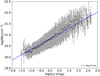 |
Fig. 8 Distribution of |
![Mathematical equation: $\[N_{\mathrm{H}}^X\]$](/articles/aa/full_html/2024/08/aa49374-24/aa49374-24-eq46.png)
![Mathematical equation: $\[N_{\mathrm{H}}^X\]$](/articles/aa/full_html/2024/08/aa49374-24/aa49374-24-eq47.png)
6 Neutral absorption density laws
Using the equivalent column densities derived from the X-ray fits, the neutral gas distribution can be modeled according to the equation
![Mathematical equation: $\[N_{\mathrm{H}}^X\left(\boldsymbol{r}_{\text {source }}\right)=\int_{\boldsymbol{r}_{\text {obeserer }}}^{\boldsymbol{r}_{\text {source }}} n(\boldsymbol{r}) \mathrm{d} \boldsymbol{r},\]$](/articles/aa/full_html/2024/08/aa49374-24/aa49374-24-eq56.png) (2)
(2)
where rsource is the distance along the line of sight to a given source and n(r) is the density law of the neutral gas in the Milky Way. First, we assumed the simplest possible model, which consists of a very thin disk for which column densities will follow a simple law ![Mathematical equation: $\[N_{\mathrm{H}}^X=N_{\mathrm{Z}} /|\sin (b)|\]$](/articles/aa/full_html/2024/08/aa49374-24/aa49374-24-eq58.png) , where b is the Galactic latitude and NZ is the vertically integrated disk column density. Figure 11 shows the values of
, where b is the Galactic latitude and NZ is the vertically integrated disk column density. Figure 11 shows the values of ![Mathematical equation: $\[N_{\mathrm{Z}}=N_{\mathrm{H}}^X|\sin (b)|\]$](/articles/aa/full_html/2024/08/aa49374-24/aa49374-24-eq59.png) as a function of |b|. We found a mean value of NZ = 1.93 × 1020 cm−2 (indicated by the horizontal blue line). Although we have identified a strong dependence of
as a function of |b|. We found a mean value of NZ = 1.93 × 1020 cm−2 (indicated by the horizontal blue line). Although we have identified a strong dependence of ![Mathematical equation: $\[N_{\mathrm{H}}^X\]$](/articles/aa/full_html/2024/08/aa49374-24/aa49374-24-eq60.png) on b (Fig. 6), the plot shows small differences in NZ, indicating that an infinitely thin disk model can be appropriated. This was expected because we are modeling column densities within the Galactic plane but at large distances from the Galactic center. Indeed, the minimum distance between the sources in our sample and the center of the Milky Way is ~5380 pc.
on b (Fig. 6), the plot shows small differences in NZ, indicating that an infinitely thin disk model can be appropriated. This was expected because we are modeling column densities within the Galactic plane but at large distances from the Galactic center. Indeed, the minimum distance between the sources in our sample and the center of the Milky Way is ~5380 pc.
We tested different density models to determine whether we could obtain constraints in the density law parameters. Given that most of the ISM radial profiles are better described in cylindrical coordinates, we defined the Galactocentric coordinates (R, z) as
![Mathematical equation: $\[R^2=r^2 \cos ^2(b)-2 r R_{\odot} \cos (b) \cos (l)+R_{\odot}^2\]$](/articles/aa/full_html/2024/08/aa49374-24/aa49374-24-eq61.png) (3)
(3)
![Mathematical equation: $\[z=r \sin (b),\]$](/articles/aa/full_html/2024/08/aa49374-24/aa49374-24-eq62.png) (4)
(4)
where R⊙ is the distance between the Sun and the Galactic center. We tested a family of density profiles commonly used to model the cold gas contribution in the Milky Way.
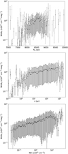 |
Fig. 10 Distribution of the |
![Mathematical equation: $\[N_{\mathrm{H}}^X / A_{\mathrm{V}}\]$](/articles/aa/full_html/2024/08/aa49374-24/aa49374-24-eq63.png)
![Mathematical equation: $\[N_{\mathrm{H}}^X\]$](/articles/aa/full_html/2024/08/aa49374-24/aa49374-24-eq64.png)
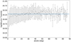 |
Fig. 11 X-ray column densities multiplied by the |sin(b)| as a function of |b|. The horizontal blue line indicates the mean value. In an infinitely thin disk model, such a product should be the same for all sources. |
-
Model A: as described by Robin et al. (2003),
![Mathematical equation: $\[n_A(R, z)=n_0 \times \exp \left(\frac{R}{h_{\mathrm{R}}}\right) \times \exp \left(-\frac{|z|}{h_z}\right),\]$](/articles/aa/full_html/2024/08/aa49374-24/aa49374-24-eq65.png) (5)
(5)where the central density (n0), the core radius (hR), and the core height (hz) are the free parameters of the model.
-
Model B: as described by Marinacci et al. (2010),
![Mathematical equation: $\[n_{\mathrm{B}}(R, z)=n_0\left(1+\frac{R}{R_{\mathrm{g}}}\right)^\gamma \times \exp ^{-R / R_{\mathrm{g}}} \times \operatorname{sech}^2\left(\frac{z}{h_{\mathrm{g}}}\right),\]$](/articles/aa/full_html/2024/08/aa49374-24/aa49374-24-eq66.png) (6)
(6)where the scale height, hg, depends on R as
![Mathematical equation: $\[h_{\mathrm{g}}(R)=h_0+\left(\frac{R}{h_{\mathrm{R}}}\right)^\delta.\]$](/articles/aa/full_html/2024/08/aa49374-24/aa49374-24-eq67.png) (7)
(7)The free parameters of the model are the central density (n0), the core radius (Rg), the slope (γ), and the scale height parameters (hR, hR, and h0).
-
Model C: as described by Marasco et al. (2013),
![Mathematical equation: $\[n_C(R, z)=n_0\left(1+\frac{R}{R_{\mathrm{g}}}\right)^\gamma \times \exp ^{-R / R_{\mathrm{g}}} \times \exp ^{-z / h_{\mathrm{g}}},\]$](/articles/aa/full_html/2024/08/aa49374-24/aa49374-24-eq68.png) (8)
(8)where the scale height, hg, is defined as Eq. (7). The free parameters of the model are the central density (n0), the core radius (Rg), the slope (γ), and the scale height parameters (hR, hR, and h0).
-
Model D: as described by Barros et al. (2016),
![Mathematical equation: $\[n_D(R, z)=\frac{n(R)}{2.12 z_0} \times \exp \left[-\left(\frac{z}{1.18 z_0}\right)^2\right],\]$](/articles/aa/full_html/2024/08/aa49374-24/aa49374-24-eq69.png) (9)
(9)with n(R) described as
![Mathematical equation: $\[\rho(R)=n_0 \times \exp \left[-\frac{\left(R^{3 / 2}-R_0^{3 / 2}\right)}{R_{0^{\prime}}^{3 / 2}}-R_{0^{\prime \prime}}\left(\frac{1}{R^2}-\frac{1}{R_0^2}\right)\right].\]$](/articles/aa/full_html/2024/08/aa49374-24/aa49374-24-eq70.png) (10)
(10)The free parameters of the model are the central density (n0), the core radius parameters (R0, R0′, R0″), and the core height (z0).
Table 1Density laws best-fit parameters.
-
Model E: as described by Nicastro et al. (2016b),
![Mathematical equation: $\[n_E(R, z)=n_0 \times \exp \left(-\sqrt{\left(R / h_{\mathrm{R}}\right)^2+\left(z / h_z\right)^2}\right).\]$](/articles/aa/full_html/2024/08/aa49374-24/aa49374-24-eq71.png) (11)
(11)The free parameters of the model are the central density (n0), the core radius (Rc), and the core height (hz).
-
Model F: as described by Gatuzz et al. (2018),
![Mathematical equation: $\[n_F(R, z)=n_0 \times \exp ~\left(-R / h_{\mathrm{R}}\right)+\exp ~\left(-|z| / h_z\right).\]$](/articles/aa/full_html/2024/08/aa49374-24/aa49374-24-eq72.png) (12)
(12)The free parameters of the model are the central density (n0), the core radius (Rc), and the core height (hz).
For each model, the parameters changed and then a Pearson chi-squared test was calculated according to the formula
![Mathematical equation: $\[\chi^2=\sum_{i=1}^N \frac{\left(N_{\mathrm{H}}^{X, i}-N_{\mathrm{H}}^{n, i}\right)^2}{\sigma_{\mathrm{X}, i}^2},\]$](/articles/aa/full_html/2024/08/aa49374-24/aa49374-24-eq73.png) (13)
(13)
where ![Mathematical equation: $\[N_{\mathrm{H}}^{X, i}\]$](/articles/aa/full_html/2024/08/aa49374-24/aa49374-24-eq74.png) is the measured column density from the X-ray observations,
is the measured column density from the X-ray observations, ![Mathematical equation: $\[N_{\mathrm{H}}^{n, i}\]$](/articles/aa/full_html/2024/08/aa49374-24/aa49374-24-eq75.png) is the expected column density value from the analytical profiles, σX,i is the column density uncertainty, and 1 ≤ i ≤ N indicates the source. In order to fit the data with such models, we need sources near the Galactic center. Therefore, we included the hydrogen column densities obtained by Gatuzz et al. (2018) for Galactic sources to obtain a better constraint on the best-fit parameters.
is the expected column density value from the analytical profiles, σX,i is the column density uncertainty, and 1 ≤ i ≤ N indicates the source. In order to fit the data with such models, we need sources near the Galactic center. Therefore, we included the hydrogen column densities obtained by Gatuzz et al. (2018) for Galactic sources to obtain a better constraint on the best-fit parameters.
Table 1 shows the best-fit parameters and the χ2 value obtained for each density profile. Figure 12 compares the predicted and measured column densities. As was mentioned before, it is important to note that we are modeling the local ISM around the Sun, and our sample lacks sources near the Galactic center. Also, the density profiles predict a smooth distribution of the column densities over the sky. At the same time, 21 cm observations indicate substantial intensity variations on different angular scales. Therefore, we can expect relatively weak constraints in the radial scale (Rc) and on the central density (as is seen by the dispersion of these parameters between the models). All best fits lead to a best-fit statistic red-χ2 ~ 2, although Model D performs slightly better. However, we note that the thickness of the disk (hz) tends to be well constrained among different models, with values in the 9 < hz < 14 pc range, in good agreement with the values obtained by Gatuzz et al. (2018) in their analysis of the X-ray ISM absorption using Galactic and extragalactic sources. We also tested fitting the data by fixing the radial scale parameters, and we have found similar values for the other parameters. Finally, we noted that fitting the data without the Gatuzz et al. (2018) values, the best-fit red-χ2 is typically about 5.
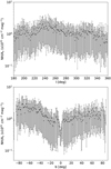 |
Fig. 9 Distribution of the |
![Mathematical equation: $\[N_{\mathrm{H}}^X / A_{\mathrm{V}}\]$](/articles/aa/full_html/2024/08/aa49374-24/aa49374-24-eq57.png)
7 Three-dimensional mapping of the interstellar medium neutral absorption
To construct a 3D density map of neutral absorption in the local ISM, we adopted the methodology outlined by Dharmawardena et al. (2022). This approach employs a Gaussian process (GP) to predict hydrogen densities based on hydrogen column densities observed along multiple lines of sight, in combination with variational inference. The process involves obtaining measurements and uncertainties of absorption toward a sample of stellar sources, along with their 3D positions. Subsequently, the logarithm of the density (log10(n)) is modeled to ensure positivity and incorporate a GP prior, accounting for correlations among densities in 3D. The posterior in log10(n) is approximated as a normal distribution, with the prior on log10(n) modeled using a GP with a constant mean.
As is described in Dharmawardena et al. (2022), the GP hyperparameters include three physical scale lengths in Heliocentric Cartesian coordinates (x, y, z) of the physical space, the mean density, and an exponential scale factor. These hyperparameters generate the GP prior, from which sets of priors are predicted. The scale factor on the prior represents the variance in the underlying Gaussian distribution from which function values are obtained. The GP is evaluated on a grid in Galactic coordinates (l, b, d) to facilitate line-of-sight integration. The coordinates of the grid cell centers are then transformed into x, y, z coordinates. To facilitate comparison with observed hydrogen column densities, the density is integrated along the line of sight by exponentiating the distribution of priors to obtain n. Subsequently, numerical integration along the line of sight to all observed coronal sources yields integrated densities, which are compared to observed column densities through likelihood optimization of the model. The optimization process refines hydrogen density as a function of position. This hierarchical approach treats the GP as a prior on (the logarithm of) hydrogen column density, whose plausible values are determined by the hyper-parameters. The algorithm is implemented using the probabilistic programming package Pyro (Phan et al. 2019) and the GPyTorch package (Gardner et al. 2021), which are both built upon the PyTorch (Paszke et al. 2019) machine learning framework. The source code has been adapted to directly work with hydrogen column densities instead of the dust extinction density.
We divided the sample into different regions for which the GP was applied to optimize the calculation. As ~92% of the sources lie at distances below <500 pc, we divided the physical space into three layers up to such a distance (see Fig. 3). The model setup also encompassed crucial parameters, including the learning rate (0.01), number of iterations (1000), number of inducing points (1000), initial scale lengths (x, y, z) = (50, 50, 50) pc, and number of cells for the grid of (x, y, z) = (110, 110, 110). Initially, we set the mean density to the values found by Gatuzz et al. (2018, n = 10−4 cm−3). For the initial scale length values, we fit a Gaussian to the distribution of separation between the input sources, obtaining a value of ~50 pc. The learning rate, number of iterations, and number of inducing points were taken from Dharmawardena et al. (2022). We selected an initial scale factor of log10(Scale factor)=−1 to account for density variations on small scales. We found that a larger number of iterations and inducing points does not improve the modeling, while significantly increasing the computing time. The number of cells for the grid in (x, y, z) is set to have a convergence of the evidence lower bound (ELBO) in a reasonable computational time, with the evidence being the integral of the likelihood over all possible parameter values (see Dharmawardena et al. 2022, for a detailed description). For example, Fig. 13 shows the variation and convergence of ELBO for the model run for Region 1. The variations in ELBO over the last iteration are below the 1% level, indicating that the model converges. As is described by Dharmawardena et al. (2022), Pyro seeks to minimize −1×ELBO instead of directly maximizing ELBO as it reports ELBO as a loss function, and therefore the y axis is positive instead of negative. The geometrical boundaries and number of sources for each region, along with the scale length, mean density, and scale factor derived from the GP analysis, are detailed in Table 2. The GP hyper-parameters obtained are within the range found by Dharmawardena et al. (2022), in their analysis of Galactic molecular clouds and complex. Figure 14 presents the hydrogen density map sampled at varying distances, akin to a computerized axial tomography. Multiple beams and clouds of diverse sizes are evident along all lines of sight, indicative of small-scale structures. The color scale represents densities ranging from n = 0 cm−3 to approximately 90 cm−3. We also attempted to create density maps for distances larger than 500 pc; however, the reduced number of sources results in a density map lacking distinct structures, becoming nearly homogeneous. Extrapolating the density profile distribution without a reliable estimate is unfeasible in such scenarios.
A substantial horizontal cloud with high density is discernible at around 100 pc, which is also observed in Fig. 5, corresponding to the region with the highest source density in our sample (refer to Fig. 2). Notably, a similar feature has been identified in previous maps of dust reddening and could potentially associated be with the local bubble or the Galactic Perseus Arm (e.g., Green et al. 2019).
We also studied a complex of three molecular clouds analyzed in Dharmawardena et al. (2023); namely, Orion (located at 180 ≤ l ≤ 217, −25.5 ≤ b ≤ −3.8, and 250 pc ≤ d ≤ 550 pc), Chameleon (290 ≤ l ≤ 308, −22 ≤ b ≤ −10, and 50 pc ≤ d ≤ 300 pc), and Coalsack (295 ≤ l ≤ 315, −4 ≤ b ≤ 4, and 50 pc ≤ d ≤ 260 pc). Figure 15 shows the predicted integrated density for each one. The highlighted regions indicate the main features associated with the complex identified by Dharmawardena et al. (2023). For the Coalsack molecular cloud, we identified the large region located at l < 302, with hints of a second high-density region at l > 304, which is also present in Dharmawardena et al. (2023), although it is more diffuse in our map. Notably, our density map also reveals the low-density region between both peaks. For the Chameleon molecular cloud, we recover the high-density peaks associated with both Cham I and Cham II and III regions. The small-scale structures observe in Dharmawardena et al. (2023), similar to a spider web, cannot be recovered, most likely due to the smaller spatial scale obtained in their analysis. In the case of Orion, we can recover the high-density peak associated with Orion B, the λ Ori structure, and there are hints of the presence of Filament λ. However, the high-density peak associated with Orion A cannot be identified in our density map. It must be noted that, due to the limited number of sources in these specific regions, a direct comparison with the results obtained by Dharmawardena et al. (2022, 2023) cannot be performed (i.e., the number of sources associated with the molecular cloud complex in our sample is ~4 times lower than them). Observational constraints, as is demonstrated in our analysis, are vital for comparisons with high-resolution 3D hydrodynamical simulations conducted in recent decades (e.g., de Avillez 2000; de Avillez & Berry 2001; Gent et al. 2013; Lagos et al. 2013; Hirschmann et al. 2016).
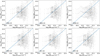 |
Fig. 12 Comparison between the measured and model-predicted column densities for the different density laws described in Sect. 6. It is clear that none of the models can reproduce the full complexity of the measurements. |
Summary of Gaussian process parameters.
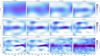 |
Fig. 14 Normalized hydrogen density map sampled at the indicated distances. |
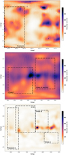 |
Fig. 15 Predicted integrated density of the Coalsack (top panel), Chameleon (middle panel), and Orion (bottom panel) molecular cloud complex. The highlighted regions indicate the main features associated with the complex identified by Dharmawardena et al. (2023). |
8 Summary and conclusions
Using the X-ray absorption technique, we have performed a detailed study of the hydrogen density distribution in the local ISM. First, hydrogen column densities were measured by fitting X-ray spectra from coronal sources identified during the inaugural eROSITA all-sky survey (eRASS1). Accurate distance measurements were obtained from Gaia DR3 for these sources. The spectral fitting involved multiple models representing the most commonly observed spectral shapes, with the final column density (![Mathematical equation: $\[N_{\mathrm{H}}^X\]$](/articles/aa/full_html/2024/08/aa49374-24/aa49374-24-eq76.png) ) selected from the model yielding the best-fit statistic. Notably, multi-temperature component models were often found to provide the best fit, underscoring the complexity of coronal spectra modeling.
) selected from the model yielding the best-fit statistic. Notably, multi-temperature component models were often found to provide the best fit, underscoring the complexity of coronal spectra modeling.
Our analysis encompasses 8231 sources, a sample size larger than previous studies, covering distances up to 4 kpc. Surprisingly, no apparent correlation emerges between column densities and distances or Galactic longitude. However, a robust correlation with Galactic latitude suggests a decrease in interstellar material density along the vertical axis moving away from the Galactic plane. A comparison with 21 cm measurements reveals instances of high-density points where ![Mathematical equation: $\[N_{\mathrm{H}}^X\]$](/articles/aa/full_html/2024/08/aa49374-24/aa49374-24-eq77.png) values tended to be lower than
values tended to be lower than ![Mathematical equation: $\[N_{\mathrm{H}}^{21 \mathrm{cm}}\]$](/articles/aa/full_html/2024/08/aa49374-24/aa49374-24-eq78.png) , potentially influenced by factors like differing effective beam sizes or the presence of absorbers beyond atomic hydrogen.
, potentially influenced by factors like differing effective beam sizes or the presence of absorbers beyond atomic hydrogen.
Further, we compared column densities and extinction values obtained from the SDSS red filter (6231 Å) along various lines of sight. We computed a slope of M = (4.82 ± 0.08) × 1021 cm−2 mag−1 between both quantities, in good agreement with previous X-ray absorption analysis but larger than Galactic extinction studies. Compared with previous studies, it is important to note that our sample is larger, covers high Galactic latitudes, and does not include SNRs, XBs, and PNe. It thus avoids intrinsic absorption, which may affect the measurements. While no clear indication of variations along the Galactic longitude for the ![Mathematical equation: $\[N_{\mathrm{H}}^X / A_{\mathrm{V}}\]$](/articles/aa/full_html/2024/08/aa49374-24/aa49374-24-eq79.png) ratio is observed, the value decreases moving toward the Galactic plane. Using equivalent column densities derived from X-ray fits, we modeled the neutral gas distribution with multiple density laws, providing a range of height scale values (9 < hz < 14 pc).
ratio is observed, the value decreases moving toward the Galactic plane. Using equivalent column densities derived from X-ray fits, we modeled the neutral gas distribution with multiple density laws, providing a range of height scale values (9 < hz < 14 pc).
Subsequently, employing the hierarchical approach elucidated in Dharmawardena et al. (2022), we inferred the hydrogen density distribution from the hydrogen column densities to generate a 3D map of neutral gas in the ISM covering distances up to 500 pc. This approach used a GP to model the log10(n) distribution, with hyperparameters including physical scale lengths in Cartesian coordinates, mean density, and an exponential scale factor. Our findings reveal the presence of multiple beams and clouds of varying sizes, indicating the existence of small-scale structures. Large dense regions around 100 pc, previously identified in dust-reddening studies, may be associated with the Galactic Perseus arm or the local bubble. Additionally, high-density regions proximal to the Orion, Chamaeleon, and Coalsack molecular complex were identified. This work underscores the capability of the X-ray absorption technique to unveil the morphological features of the local ISM.
Acknowledgements
This work is based on data from eROSITA, the soft X-ray instrument aboard SRG, a joint Russian-German science mission supported by the Russian Space Agency (Roskosmos), in the interests of the Russian Academy of Sciences represented by its Space Research Institute (IKI), and the Deutsches Zentrum für Luft- und Raumfahrt (DLR). The SRG spacecraft was built by Lavochkin Association (NPOL) and its subcontractors, and is operated by NPOL with support from the Max Planck Institute for Extraterrestrial Physics (MPE). The development and construction of the eROSITA X-ray instrument was led by MPE, with contributions from the Dr. Karl Remeis Observatory Bamberg & ECAP (FAU Erlangen-Nuernberg), the University of Hamburg Observatory, the Leibniz Institute for Astrophysics Potsdam (AIP), and the Institute for Astronomy and Astrophysics of the University of Tübingen, with the support of DLR and the Max Planck Society. The Argelander Institute for Astronomy of the University of Bonn and the Ludwig Maximilians Universität Munich also participated in the science preparation for eROSITA. This research was carried out on the High Performance Computing resources of the cobra cluster at the Max Planck Computing and Data Facility (MPCDF) in Garching operated by the Max Planck Society (MPG). The eROSITA data shown here were processed using the eSASS software system developed by the German eROSITA consortium. PCS acknowledges support from DLR through grant 50OR2102.
References
- Bajaja, E., Arnal, E. M., Larrarte, J. J., et al. 2005, A&A, 440, 767 [NASA ADS] [CrossRef] [EDP Sciences] [Google Scholar]
- Barros, D. A., Lépine, J. R. D., & Dias, W. S. 2016, A&A, 593, A108 [NASA ADS] [CrossRef] [EDP Sciences] [Google Scholar]
- Churazov, E., Gilfanov, M., Forman, W., & Jones, C. 1996, ApJ, 471, 673 [NASA ADS] [CrossRef] [Google Scholar]
- Coffaro, M., Stelzer, B., & Orlando, S. 2022, A&A, 661, A79 [NASA ADS] [CrossRef] [EDP Sciences] [Google Scholar]
- Dame, T. M., Hartmann, D., & Thaddeus, P. 2001, ApJ, 547, 792 [Google Scholar]
- de Avillez, M. A. 2000, MNRAS, 315, 479 [NASA ADS] [CrossRef] [Google Scholar]
- de Avillez, M. A., & Berry, D. L. 2001, MNRAS, 328, 708 [NASA ADS] [CrossRef] [Google Scholar]
- Dharmawardena, T. E., Bailer-Jones, C. A. L., Fouesneau, M., & Foreman-Mackey, D. 2022, A&A, 658, A166 [NASA ADS] [CrossRef] [EDP Sciences] [Google Scholar]
- Dharmawardena, T. E., Bailer-Jones, C. A. L., Fouesneau, M., et al. 2023, MNRAS, 519, 228 [Google Scholar]
- Dickey, J. M., & Lockman, F. J. 1990, ARA&A, 28, 215 [Google Scholar]
- Draine, B. T. 2011, Physics of the Interstellar and Intergalactic Medium (Princeton University Press) [CrossRef] [Google Scholar]
- Eckersall, A. J., Vaughan, S., & Wynn, G. A. 2017, MNRAS, 471, 1468 [NASA ADS] [CrossRef] [Google Scholar]
- Foight, D. R., Güver, T., Özel, F., & Slane, P. O. 2016, ApJ, 826, 66 [Google Scholar]
- Freund, S., Czesla, S., Robrade, J., Schneider, P. C., & Schmitt, J. H. M. M. 2022, A&A, 664, A105 [NASA ADS] [CrossRef] [EDP Sciences] [Google Scholar]
- Freund, S., Czesla, S., Predehl, P., et al. 2024, A&A, 684, A121 [NASA ADS] [CrossRef] [EDP Sciences] [Google Scholar]
- Gaia Collaboration (Brown, A. G. A., et al.) 2021, A&A, 649, A1 [NASA ADS] [CrossRef] [EDP Sciences] [Google Scholar]
- Gaia Collaboration (Vallenari, A., et al.) 2023, A&A, 674, A1 [NASA ADS] [CrossRef] [EDP Sciences] [Google Scholar]
- Gardner, J. R., Pleiss, G., Bindel, D., Weinberger, K. Q., & Wilson, A. G. 2021, GPyTorch: Blackbox Matrix-Matrix Gaussian Process Inference with GPU Acceleration [Google Scholar]
- Gatuzz, E., & Churazov, E. 2018, MNRAS, 474, 696 [NASA ADS] [CrossRef] [Google Scholar]
- Gatuzz, E., García, J., Mendoza, C., et al. 2013a, ApJ, 778, 83 [CrossRef] [Google Scholar]
- Gatuzz, E., García, J., Mendoza, C., et al. 2013b, ApJ, 768, 60 [NASA ADS] [CrossRef] [Google Scholar]
- Gatuzz, E., García, J., Mendoza, C., et al. 2014, ApJ, 790, 131 [NASA ADS] [CrossRef] [Google Scholar]
- Gatuzz, E., García, J., Kallman, T. R., Mendoza, C., & Gorczyca, T. W. 2015, ApJ, 800, 29 [NASA ADS] [CrossRef] [Google Scholar]
- Gatuzz, E., García, J. A., Kallman, T. R., & Mendoza, C. 2016, A&A, 588, A111 [NASA ADS] [CrossRef] [EDP Sciences] [Google Scholar]
- Gatuzz, E., Rezaei, K. S., Kallman, T. R., et al. 2018, MNRAS, 479, 3715 [CrossRef] [Google Scholar]
- Gatuzz, E., Díaz Trigo, M., Miller-Jones, J. C. A., & Migliari, S. 2019, MNRAS, 482, 2597 [Google Scholar]
- Gatuzz, E., Díaz Trigo, M., Miller-Jones, J. C. A., & Migliari, S. 2020a, MNRAS, 491, 4857 [CrossRef] [Google Scholar]
- Gatuzz, E., Gorczyca, T. W., Hasoglu, M. F., et al. 2020b, MNRAS, 498, L20 [NASA ADS] [CrossRef] [Google Scholar]
- Gatuzz, E., García, J. A., & Kallman, T. R. 2021, MNRAS, 504, 4460 [NASA ADS] [CrossRef] [Google Scholar]
- Gent, F. A., Shukurov, A., Fletcher, A., Sarson, G. R., & Mantere, M. J. 2013, MNRAS, 432, 1396 [NASA ADS] [CrossRef] [Google Scholar]
- Green, G. 2018, J. Open Source Softw., 3, 695 [NASA ADS] [CrossRef] [Google Scholar]
- Green, G. M., Schlafly, E. F., Finkbeiner, D., et al. 2018, MNRAS, 478, 651 [Google Scholar]
- Green, G. M., Schlafly, E., Zucker, C., Speagle, J. S., & Finkbeiner, D. 2019, ApJ, 887, 93 [NASA ADS] [CrossRef] [Google Scholar]
- Grevesse, N., & Sauval, A. J. 1998, Space Sci. Rev., 85, 161 [Google Scholar]
- Güver, T., & Özel, F. 2009, MNRAS, 400, 2050 [Google Scholar]
- Hartmann, D., & Burton, W. B. 1997, Atlas of Galactic Neutral Hydrogen (Cambridge: Cambridge University Press), 243 [Google Scholar]
- Hirschmann, M., De Lucia, G., & Fontanot, F. 2016, MNRAS, 461, 1760 [Google Scholar]
- Joachimi, K., Gatuzz, E., García, J. A., & Kallman, T. R. 2016, MNRAS, 461, 352 [NASA ADS] [CrossRef] [Google Scholar]
- Juett, A. M., Schulz, N. S., & Chakrabarty, D. 2004, ApJ, 612, 308 [NASA ADS] [CrossRef] [Google Scholar]
- Juett, A. M., Schulz, N. S., Chakrabarty, D., & Gorczyca, T. W. 2006, ApJ, 648, 1066 [NASA ADS] [CrossRef] [Google Scholar]
- Kalberla, P. M. W., Burton, W. B., Hartmann, D., et al. 2005, A&A, 440, 775 [NASA ADS] [CrossRef] [EDP Sciences] [Google Scholar]
- Lagos, C. d. P., Lacey, C. G., & Baugh, C. M. 2013, MNRAS, 436, 1787 [NASA ADS] [CrossRef] [Google Scholar]
- Liao, J.-Y., Zhang, S.-N., & Yao, Y. 2013, ApJ, 774, 116 [NASA ADS] [CrossRef] [Google Scholar]
- Marasco, A., Marinacci, F., & Fraternali, F. 2013, MNRAS, 433, 1634 [NASA ADS] [CrossRef] [Google Scholar]
- Marinacci, F., Fraternali, F., Ciotti, L., & Nipoti, C. 2010, MNRAS, 401, 2451 [CrossRef] [Google Scholar]
- Merloni, A., Lamer, G., Liu, T., et al. 2024, A&A, 682, A34 [NASA ADS] [CrossRef] [EDP Sciences] [Google Scholar]
- Nicastro, F., Senatore, F., Gupta, A., et al. 2016a, MNRAS, 457, 676 [NASA ADS] [CrossRef] [Google Scholar]
- Nicastro, F., Senatore, F., Krongold, Y., Mathur, S., & Elvis, M. 2016b, ApJ, 828, L12 [NASA ADS] [CrossRef] [Google Scholar]
- Paszke, A., Gross, S., Massa, F., et al. 2019, PyTorch: An Imperative Style, High-Performance Deep Learning Library [Google Scholar]
- Phan, D., Pradhan, N., & Jankowiak, M. 2019, Composable Effects for Flexible and Accelerated Probabilistic Programming in NumPyro [Google Scholar]
- Pinto, C., Kaastra, J. S., Costantini, E., & Verbunt, F. 2010, A&A, 521, A79 [NASA ADS] [CrossRef] [EDP Sciences] [Google Scholar]
- Pinto, C., Kaastra, J. S., Costantini, E., & de Vries, C. 2013, A&A, 551, A25 [NASA ADS] [CrossRef] [EDP Sciences] [Google Scholar]
- Predehl, P., & Schmitt, J. H. M. M. 1995, A&A, 293, 889 [NASA ADS] [Google Scholar]
- Predehl, P., Andritschke, R., Arefiev, V., et al. 2021, A&A, 647, A1 [EDP Sciences] [Google Scholar]
- Psaradaki, I., Costantini, E., Mehdipour, M., et al. 2020, A&A, 642, A208 [NASA ADS] [CrossRef] [EDP Sciences] [Google Scholar]
- Rezaei Kh., S., Bailer-Jones, C. A. L., Hanson, R. J., & Fouesneau, M. 2017, A&A, 598, A125 [NASA ADS] [CrossRef] [EDP Sciences] [Google Scholar]
- Robin, A. C., Reylé, C., Derrière, S., & Picaud, S. 2003, A&A, 409, 523 [NASA ADS] [CrossRef] [EDP Sciences] [Google Scholar]
- Robrade, J., Schmitt, J. H. M. M., & Favata, F. 2012, A&A, 543, A84 [NASA ADS] [CrossRef] [EDP Sciences] [Google Scholar]
- Sancisi, R., Fraternali, F., Oosterloo, T., & van der Hulst, T. 2008, A&A Rev., 15, 189 [CrossRef] [Google Scholar]
- Schlafly, E. F., & Finkbeiner, D. P. 2011, ApJ, 737, 103 [Google Scholar]
- Schlegel, D. J., Finkbeiner, D. P., & Davis, M. 1998, ApJ, 500, 525 [Google Scholar]
- Schneider, P. C., Freund, S., Czesla, S., et al. 2022, A&A, 661, A6 [NASA ADS] [CrossRef] [EDP Sciences] [Google Scholar]
- Schulz, N. S., Cui, W., Canizares, C. R., et al. 2002, ApJ, 565, 1141 [CrossRef] [Google Scholar]
- Takei, Y., Fujimoto, R., Mitsuda, K., & Onaka, T. 2002, ApJ, 581, 307 [CrossRef] [Google Scholar]
- Valencic, L. A., & Smith, R. K. 2015, ApJ, 809, 66 [NASA ADS] [CrossRef] [Google Scholar]
- Watson, D. 2011, A&A, 533, A16 [CrossRef] [EDP Sciences] [Google Scholar]
- Weingartner, J. C., & Draine, B. T. 2001, ApJ, 548, 296 [Google Scholar]
- Willingale, R., Starling, R. L. C., Beardmore, A. P., Tanvir, N. R., & O’Brien, P. T. 2013, MNRAS, 431, 394 [Google Scholar]
- Wilms, J., Allen, A., & McCray, R. 2000, ApJ, 542, 914 [Google Scholar]
- Winkel, B., Kerp, J., Flöer, L., et al. 2016, A&A, 585, A41 [NASA ADS] [CrossRef] [EDP Sciences] [Google Scholar]
- Yao, Y., Schulz, N. S., Gu, M. F., Nowak, M. A., & Canizares, C. R. 2009, ApJ, 696, 1418 [NASA ADS] [CrossRef] [Google Scholar]
- Zhu, H., Tian, W., Li, A., & Zhang, M. 2017, MNRAS, 471, 3494 [NASA ADS] [CrossRef] [Google Scholar]
All Tables
All Figures
|
Fig. 1 Distribution of the 8231 eRASS1 sources analyzed in this work. |
| In the text | |
|
Fig. 2 Distribution of sources as a function of different parameters. Top panel: distribution of sources as a function of the number of counts in the 0.2–10 keV energy range. Bottom panel: distribution of sources as a function of the distance obtained from the Gaia observatory. |
| In the text | |
|
Fig. 3 Distribution of the sources for different distance ranges in Aitoff projection. The colors indicate the log( |
| In the text | |
|
Fig. 4
|
| In the text | |
|
Fig. 5
|
| In the text | |
|
Fig. 6
|
| In the text | |
|
Fig. 7 Comparison between |
| In the text | |
|
Fig. 8 Distribution of |
| In the text | |
|
Fig. 9 Distribution of the |
| In the text | |
|
Fig. 10 Distribution of the |
| In the text | |
|
Fig. 11 X-ray column densities multiplied by the |sin(b)| as a function of |b|. The horizontal blue line indicates the mean value. In an infinitely thin disk model, such a product should be the same for all sources. |
| In the text | |
|
Fig. 12 Comparison between the measured and model-predicted column densities for the different density laws described in Sect. 6. It is clear that none of the models can reproduce the full complexity of the measurements. |
| In the text | |
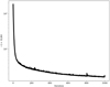 |
Fig. 13 Variation in ELBO through model iterations for Region 1 in Table 2. |
| In the text | |
|
Fig. 14 Normalized hydrogen density map sampled at the indicated distances. |
| In the text | |
|
Fig. 15 Predicted integrated density of the Coalsack (top panel), Chameleon (middle panel), and Orion (bottom panel) molecular cloud complex. The highlighted regions indicate the main features associated with the complex identified by Dharmawardena et al. (2023). |
| In the text | |
Current usage metrics show cumulative count of Article Views (full-text article views including HTML views, PDF and ePub downloads, according to the available data) and Abstracts Views on Vision4Press platform.
Data correspond to usage on the plateform after 2015. The current usage metrics is available 48-96 hours after online publication and is updated daily on week days.
Initial download of the metrics may take a while.