| Issue |
A&A
Volume 683, March 2024
|
|
|---|---|---|
| Article Number | A213 | |
| Number of page(s) | 6 | |
| Section | Extragalactic astronomy | |
| DOI | https://doi.org/10.1051/0004-6361/202348705 | |
| Published online | 20 March 2024 | |
Probing the physical properties of the intergalactic medium using SRG/eROSITA spectra from blazars
1
Max-Planck-Institut für Extraterrestrische Physik, Gießenbachstraße 1, 85748 Garching, Germany
e-mail: This email address is being protected from spambots. You need JavaScript enabled to view it.
2
Dr. Karl Remeis-Observatory & ECAP, Friedrich-Alexander-Universität Erlangen-Nürnberg, Sternwartstr. 7, 96049 Bamberg, Germany
3
Kavli Institute for Astrophysics and Space Research, Massachusetts Institute of Technology, Cambridge, MA, USA
Received:
22
November
2023
Accepted:
1
February
2024
Abstract
Most baryonic matter resides in the intergalactic medium (IGM). This diffuse gas is primarily composed of ionized hydrogen and helium and fills the space between galaxies. Observations of this environment are crucial for better understanding the physical processes in it. We present an analysis of the IGM absorption using blazar spectra from the first eROSITA all-sky survey (eRASS1) performed onboard of the Spectrum-Roentgen-Gamma mission (SRG) and XMM-Newton X-ray observations. First, we fit the continuum spectra using a log-parabolic spectrum model and fixed the Galactic absorption. Then, we included a collisional ionization equilibrium model, namely IONeq, to account for the IGM absorption. The column density N(H) and metallicity (Z) were set as free parameters. At the same time, the redshift of the absorber was fixed to half the blazar redshift as an approximation of the full line-of-sight absorber. We measured IGM-N(H) for 147 sources for SRG and 10 sources for XMM-Newton. We found a clear trend between IGM-N(H) and the blazar redshifts that scales as (1 + z)1.63 ± 0.12. The mean hydrogen density at z = 0 is n0 = (2.75 ± 0.63)×10−7 cm−3. The mean temperature over the redshift range is log(T/K) = 5.6 ± 0.6, and the mean metallicity is Z = 0.16 ± 0.09. We found no acceptable fit using a power-law model for the temperatures or metallicities as a function of the redshift. These results indicate that the IGM contributes substantially to the total absorption seen in the blazar spectra.
Key words: galaxies: high-redshift / intergalactic medium / X-rays: galaxies / X-rays: general
© The Authors 2024
 Open Access article, published by EDP Sciences, under the terms of the Creative Commons Attribution License (https://creativecommons.org/licenses/by/4.0), which permits unrestricted use, distribution, and reproduction in any medium, provided the original work is properly cited.
This article is published in open access under the Subscribe to Open model.
Open Access funding provided by Max Planck Society.
1. Introduction
The intergalactic medium (IGM) is a diffuse gas primarily composed of ionized hydrogen and helium, filling the space between galaxies within the vast cosmic structure known as the large-scale cosmic web. Most baryonic matter resides in the IGM, with a fraction even higher in the early Universe as less material coalesced gravitationally from it (McQuinn 2016). Simulations predict that up to 50% of the baryons by mass have been shock-heated into the warm-hot phase (WHIM) at low redshift (z < 2), with baryon densities nb = 10−6 − 10−4 cm−3 and temperatures T = 105 − 107 K (Cen & Ostriker 1999; Davé & Oppenheimer 2007; Schaye et al. 2015). Simulations predict that the cool diffuse IGM constitutes ∼39% of the baryons at redshift z = 0 (Martizzi et al. 2019). In this sense, observations are essential for better understanding the production, transport, and distribution of metals within the IGM.
Most ionized IGM metals are not observed in the optical to UV. Hence, X-ray absorption studies constitute a powerful technique with which this environment can be observed. Using a bright X-ray background source that acts as a lamp, we gain information from the final X-ray absorption spectra about the total absorbing column density of the material between the source and the observer. The typical sources commonly used to perform this analysis include active galactic nuclei (AGN) and gamma-ray bursts (GRBs, Galama & Wijers 2001; Watson et al. 2007; Watson 2011; Schady 2017; Nicastro et al. 2017, 2018; Dalton et al. 2021a; Gatuzz et al. 2023). When the contribution of the Galactic absorption is included, which is usually known from 21 cm measurements (e.g., Kalberla et al. 2005; Willingale et al. 2013; HI4PI Collaboration 2016), an additional absorption component is added to account for the excess absorption due to the IGM. With this technique, X-ray low-resolution spectra (i.e., charge-coupled devices) can be used to estimate the total hydrogen column density of the IGM. Future observatories, such as the Line Emission Mapper (LEM, Kraft et al. 2022) and Athena (Nandra et al. 2013), will measure X-ray high-resolution spectral features, such as lines and edges (Walsh et al. 2020).
A key finding from previous observations of the IGM using high-redshift tracers is the apparent increase in excess of N(H) with redshift (e.g., Behar et al. 2011; Watson 2011; Campana et al. 2012). One perspective postulates that the host source causes all the excess and evolution (Owens et al. 1998; Galama & Wijers 2001; Stratta et al. 2004; Campana et al. 2006, 2010; Schady et al. 2011; Watson et al. 2013; Arcodia et al. 2016; Buchner & Bauer 2017). Another perspective argues that the IGM contributes substantially to the absorption, and that it is therefore redshift related (Starling et al. 2013; Campana et al. 2015; Rahin & Behar 2019; Dalton & Morris 2020; Dalton et al. 2021b, 2022). Blazars are sources with negligible X-ray absorption along the line-of-sight (LOS) within the host galaxy. They are therefore ideal candidates for testing the absorption IGM component and the N(H)−z relation. However, only a few studies have been made with these sources (e.g., Molendi et al. 2000; Fabian et al. 2001; Worsley et al. 2004). Arcodia et al. (2018) analyzed XMM-Newton spectra of 15 blazars at z > 2. They found an average IGM hydrogen density at redshift zero of  cm−3 and a temperature of
  . Dalton et al. (2021b), on the other hand, analyzed a sample of 40 Swift blazars over a redshift range of 0.03 < z < 4.7 in combination with a subsample of 7 XMM-Newton sources. They found that the N(H) scales as (1 + z)1.8 ± 0.2, with a mean hydrogen density at z = 0 of n0 = (3.2 ± 0.5)×10−7 cm−3, a temperature of log(T/K) = 6.1 ± 0.1, and a mean metallicity of [X/H] = −1.62 ± 0.04 (Z ∼ 0.02).
Here, we present an analysis of the IGM absorption using X-ray observations of blazars taken with the SRG/eROSITA X-ray telescope. This paper is structured as follows. Section 2 provides a detailed description of the data selection. Section 3 discusses the fitting procedure we used in our analysis. We present the results in Sect. 4. We discuss and compare the results with those of other studies in Sect. 5. Finally, Sect. 6 summarizes our findings and presents our conclusions. Throughout this paper, we assumed a ΛCDM cosmology with Ωm = 0.3, ΩΛ = 0.7, and H0 = 70 km s−1 Mpc−1.
2. Data sample
The SRG/eROSITA X-ray telescope (Predehl et al. 2021) on board the Spectrum Roentgen Gamma (SRG) observatory consists of seven Wolter-I geometry X-ray telescopes providing all-sky survey observations in the 0.2 − 10 keV energy range. During the first all-sky survey (eRASS1), more than one million sources were detected by SRG/eROSITA, with AGNs accounting for 80% of the sources in the catalog (Merloni et al. 2024). An X-ray sample of blazars was created by Hämmerich et al. (in prep.) using eRASS1 data. Known blazars were taken from the 3HSP (Chang et al. 2019), ROMA BZCAT (Massaro et al. 2015), and 4FGL (Ballet et al. 2023) catalogs. By applying a cross-match with a radius of 8″, 666 BL Lac and 841 flat spectrum radio quasars (FSRQ) were identified. This is the most significant systematic X-ray sample of blazars compiled so far. This dataset constitutes the initial sample in our analysis.
The complete details of the data reduction are shown in Hämmerich et al. (in prep.). We summarize the main aspects here. We reduced the data using the SRG/eROSITA data analysis software eSASS pipeline version 020 (Brunner et al. 2022). First, we extracted the spectra using circular extraction regions with the radius scaled to the 0.2 − 2.3 keV maximum likelihood (ML) count rate from the eRASS1 source catalog. Following an empirical relation, larger radii correspond to higher count rates. Background regions were created as annuli with a size scaled to the ML count rate. eRASS1 sources located within the background region were removed using a circular region with radii depending on the ML count rate. The task srctool was used on the event files to create spectral and response files. We combined the spectra from all telescope modules (TMs).
2.1. XMM-Newton subsample
To cover z > 2 redshift regions, we added a subsample of 15 blazars analyzed by Arcodia et al. (2018) in their study of the IGM absorption. Table 1 shows the sample details, covering a redshift range up to z = 4.715. We reduced the spectra from the XMM-Newton European Photon Imaging Camera (EPIC, Strüder et al. 2001) with the Science Analysis System (SAS1, version 21.0.0). The observations were reduced with the epchain SAS tool, including single and double pixel events (i.e., PATTERN<=4) and filtering the data with FLAG==0 to avoid bad pixels and parts of the detector close to the CCD edges. Bad time intervals were filtered by using a 0.35 cts s−1 rate threshold. For all sources, the final spectra were binned to oversample the instrumental resolution by at least a factor of 3 and to have a minimum of 20 counts per channel.
List of z > 2 with XMM-Newton sample.
3. Spectral fitting
All spectra were fit using the xspec spectral fitting package (version 12.13.12). We used the cash statistics (Cash 1979). The errors are quoted at 1σ confidence level unless otherwise stated. Finally, the abundances are given relative to Grevesse & Sauval (1998). We fit the spectra in the 0.3 − 10 keV energy range. However, in the case of SRG/eROSITA, we created two groups by combining TM 1-4, 6 and TM 5, 7 because TM 5 and 7 are susceptible to excess soft emission due to optical light leaking (Predehl et al. 2021). The last one was only analyzed for energies > 1 keV. Below, we describe the spectral modeling.
3.1. Galactic absorption and continuum model
Following the detailed study by Dalton et al. (2021a), we fit each source with the model tbabs*ioneq*logpar. The tbabs component models the absorption in the local interstellar medium (ISM) as described by Wilms et al. (2000). The ISM-N(H) parameter was fixed to the Willingale et al. (2013) values, which were estimated from 21 cm radio emission maps from Kalberla et al. (2005), but including a molecular hydrogen column density component. For the continuum, we included a log-parabolic spectrum logpar, which can be produced by a log-parabolic distribution of relativistic particles (Paggi et al. 2009) or due to a power-law particle distribution with a cooled high-energy tail (Furniss et al. 2013). While a broken power-law intrinsic curvature could also arise from these environments, Arcodia et al. (2018) and Dalton et al. (2021a) found that a log-parabolic power law led to better modeling of blazar X-ray spectra. This agrees well with previous studies (e.g., Bhatta et al. 2018; Sahakyan et al. 2020).
Upper and lower limits of the free parameters considered for the IGM absorption component.
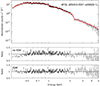 |
Fig. 1. SRG/eROSITA best-fit spectra of one of the sources included in the sample (4FGL J0543.9–5531). The black data points show the observations, and the solid red line corresponds to the best-fit model including the IGM component. The bottom panels show the data-model ratio for the models without and with the IGM component (see Sect. 3 for further details). All cameras were grouped for illustration purposes. |
3.2. IGM absorption
To model the IGM absorption, we used the IONeq model (Gatuzz & Churazov 2018), which assumes collisional ionization equilibrium (CIE) and includes as model parameters the hydrogen column density (N(H)), gas temperature (log(T/K)), metallicity (Z), turbulent broadening (vturb), and redshift (z). Thus, we assumed a thin uniform plane-parallel slab geometry in ionization equilibrium for the IGM. This approximation is commonly used for a homogeneous medium (Savage et al. 2014; Khabibullin & Churazov 2019; Lehner et al. 2019; Dalton et al. 2021a). We placed this slab at half the blazar redshift to approximate the complete line-of-sight medium. The parameter ranges applied to this model were taken from Dalton et al. (2021a) and are listed in Table 2. The range of temperatures allowed us to consider the cool IGM phase (4.5 > log(T/K) < 5, Schaye et al. 2003; Simcoe et al. 2004; Aguirre et al. 2008) and the WHIM phases (log(T/K) > 5, Danforth et al. 2016; Pratt et al. 2018). We note that the host X-ray absorption contribution in blazars is also negligible because it is swept away by the kiloparsec-scale relativistic jet (Arcodia et al. 2018; Dalton et al. 2021b). This is consistent with low optical-UV extinction levels observed in these sources (Paliya et al. 2016). Simulations show that the density is very low along the LOS to collimated outflows (Chatterjee et al. 2019). Figures 1 and 2 show examples of the best-fit results obtained for one source of the SRG/eROSITA and XMM-Newton samples. The plots are zoomed in to the soft-energy band to better illustrate the impact of adding an absorption component associated with the IGM. Finally, while a hybrid model including an absorber under photoionization equilibrium (PIE) conditions in combination with a CIE absorber would be more physical, high-resolution spectra would be necessary to test it (Dalton et al. 2021b).
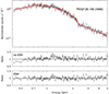 |
Fig. 2. XMM-Newton EPIC-pn best-fit spectra of one of the sources included in the sample (PKS 2126–158; see Sect. 3 for further details). |
4. Spectral analysis results
We have measured IGM-N(H) for 147 sources from the SRG/eROSITA initial sample, covering a redshift range up to z = 2.232. That is, the best-fit statistic was better when the IGM component was included than the statistic with Galactic absorption alone (ΔC-stat. > 10, as in Dalton et al. 2021b). Upper limits were obtained for 199 sources, but for the rest of sources, a statistical improvement of the fit was not found (i.e., 320 sources). For the XMM-Newton sample, we measured IGM-N(H) for 10 sources and only upper limits for 5. In the following analysis, we excluded the upper limits, which may lead to a biased understanding of the proper distribution of the absorption features. In this sense, by incorporating a parameter range into our models, we ensured a comprehensive understanding of the uncertainties associated with our findings.
4.1. IGM parameter results
Figure 3 shows the IGM-N(H) distribution as a function of the redshift obtained from the best fits. We found that a power-law fit scales as (1 + z)1.63 ± 0.12 when XMM-Newton data are included and (1 + z)2.40 ± 0.19 when only SRG/eROSITA data are fit. A fit like this is not appropriate for low-redshift values, as the plot shows. The solid blue line Fig. 3 shows the mean hydrogen density of the IGM based on the model developed in (see Starling et al. 2013; Shull & Danforth 2018; Dalton et al. 2021a, and references therein),
![Mathematical equation: $$ \begin{aligned} N_{\rm HXIGM} = \frac{n_{0}c}{H_{0}}\int _{0}^{z}\frac{(1+z)^{2}\mathrm{d}z}{[\Omega _{\rm m}(1+z)^{3}+\Omega _{\lambda }]^{\frac{1}{2}}}, \end{aligned} $$](/articles/aa/full_html/2024/03/aa48705-23/aa48705-23-eq3.gif) (1)
(1)
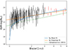 |
Fig. 3. Distribution of IGM-N(H) vs. redshift. The black points show the SRG/eROSITA sample, and the red points show the XMM-Newton sample. The blue line represents the IGM model shown in Eq. (1). The solid orange line corresponds to a power-law fit. The solid green line corresponds to the model proposed by Campana et al. (2015). |
where n0 is the hydrogen density at redshift zero, assuming that 90% of the baryons are in the IGM (Behar et al. 2011). Using Eq. (1), we found a mean hydrogen density of n0 = (2.75 ± 0.63)×10−7 cm−3 when the XMM-Newton was included, and for the fit with the SRG/eROSITA data alone, we found n0 = (4.31 ± 1.20)×10−7 cm−3. This shows that it is important to include sources at high redshift in IGM evolution studies. For comparison, Table 3 shows a list of n0 values obtained in previous works, including theoretical as well as IGM absorption measurements using blazars, quasars, and GRBs as background sources. The solid green line in Fig. 3 corresponds to the model proposed by Campana et al. (2015). This curve is obtained from the cosmological simulations presented in Pallottini et al. (2013). At low redshift, we note that multiple blazars have a larger IGM-N(H) than the mean hydrogen density model. This could be due to the presence of the circumgalactic medium (CGM) in both our Galaxy and the host galaxy, or to discrete intervening systems associated with other galaxies, thus providing more absorbing material.
n0 values in the literature.
The top panel in Fig. 4 shows the temperature distribution as a function of the blazar redshift. Black points correspond to the SRG/eROSITA data, while red points correspond to the XMM-Newton sample. The fitted temperatures scatter in the 4 < log(T/K) < 7.5 range. The mean temperature over the redshift range is log(T/K) = 5.6 ± 0.6, consistent with the cold WHIM (Tuominen et al. 2021). There is no apparent relation between the temperature and redshift due to the large scatter. Because the fits were made for the integrated LOS, they are not representative of individual absorber temperatures. The bottom panel in Fig. 4 shows the metallicity distribution as a function of the blazars redshift. The fitted metallicities scatter in the 0.1 < Z < 0.2 range at redshift z < 3 with significant uncertainties. The mean metallicity over the entire redshift range is Z = 0.16 ± 0.09, which is consistent with the WHIM component (e.g., Nicastro et al. 2018). While the metallicity tends to decrease with redshift, we did not find an acceptable fit (i.e., χ2/d.o.f. > 5) using a power-law model (i.e., (1 + z)a) for either temperatures or abundances.
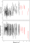 |
Fig. 4. Distribution of the best-fit parameters as function of the redshifts. Top panel: distribution of IGM-kT vs. redshift. Bottom panel: distribution of IGM-metallicity vs. redshift. The black points show the SRG/eROSITA sample, and the red points correspond to the XMM-Newton sample. |
4.2. Robustness of IGM-N(H) measurements
Various scenarios could account for the observed soft excess in blazars without necessitating IGM absorption. For example, an IGM-N(H) and spectral degeneracy might occur to some degree. A harder spectrum slope may mimic large IGM-N(H), and vice versa. We searched for a relation between the IGM-N(H) and the α index of the logpar model (see the top panel in Fig. 5) We found no apparent relation between the α indices and the column density. This is consistent with previous results (Arcodia et al. 2018; Ben Haim et al. 2019; Dalton et al. 2021a) The bottom panel in Fig. 5 shows the count rate for each source as a function of the IGM-N(H). There is no apparent relation between the two parameters. Blazars display variability due to multiple processes such as particle acceleration, injection, cooling, and escape (Gaur 2020). Any IGM absorber found in the LOS to such a system should not show variability, while a local absorber can. While eRASS1 data alone cannot be used to study variability within the sources, Dalton et al. (2021a) showed in their analysis of XMM-Newton and Swift blazar spectra that the lack of an apparent relation between IGM-N(H) and flux indicates that the absorption measured from the X-ray spectra is associated with the IGM and not with the sources. Finally, it is notable that our model relies on the assumption of a thin slab positioned at half the redshift of each source. The efficacy of this approach is contingent upon the validity of this simplifying assumption and may be subject to the specific characteristics of the observed blazar spectra. A thorough examination of this approximation across various sources and conditions with future X-ray observatories such as Athena (Nandra et al. 2013) would provide valuable insights into its robustness.
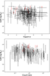 |
Fig. 5. Measurements of robustness for the IGM-N(H) measurements. Top panel: distribution of IGM-N(H) as function of the logparα indices. Bottom panel: distribution of IGM-N(H) as function of the count rates. The black points show the SRG/eROSITA sample, and the red points correspond to the XMM-Newton sample. |
5. Comparison with previous works
Even though their properties are ideally suited for studying such an environment, only a few systematic IGM absorption studies have been performed using blazars as X-ray sources. Arcodia et al. (2018) measured IGM-N(H) for a sample of 15 sources using XMM-Newton observations with a absori based XSPEC absorption model. They concluded that excess absorption is the preferred scenario to explain the N(H)−(z + 1) relation. They found an IGM gas density of (1.0 ± 0.6)×10−7 cm−3 and a temperature of  . In addition to differences in both the continuum and the absorption modeling, we note when we compared our results with theirs that they fixed the continuum powerlaw parameters when including the IGM absorber. This approach was adopted due to computational limits. More importantly, they assumed a solar abundance in their modeling. From the IGM gas density, they inferred an IGM metallicity
  , which is higher than the value obtained from our analysis. Dalton et al. (2021b) analyzed Swift spectra of 40 blazars with a redshift range of 0.03 ≤ z ≤ 4.7. They also included XMM-Newton observations of 7 blazars in the 0.86 ≤ z ≤ 3.26 range. We followed the same analysis method as described in Sect. 3. Considering the uncertainties, our n0 and metallicity values agree well with their results (see Table 3). Moreover, they found no apparent relation between the logpar index or the column density.
6. Conclusions
We studied the IGM absorption using the X-ray sample of blazars computed by Hämmerich et al. (in prep.) using eRASS1 data in combination with a XMM-Newton subsample of 15 blazars. Following the work done in Dalton et al. (2021b), we modeled the continuum with a log-parabolic spectrum model and fixed the Galactic absorption to the 21 cm values. After modeling the continuum component, we included a IONeq model, which assumes CIE conditions, to search for IGM absorbers. The column density N(H) and metallicity (Z) were set as free parameters. At the same time, the redshift of the absorber was fixed to half the blazar redshift as an approximation of the full line-of-sight absorber. From the SRG/eROSITA sample, we measured column densities (IGM-N(H)) for 147 sources, covering a redshift range up to z = 2.232, while for the XMM-Newton sample, we measured IGM-N(H) for 10 sources. We found a clear trend between IGM-N(H) and the blazar redshifts, which can be modeled with a mean hydrogen density model with n0 = (2.75 ± 0.63)×10−7 cm−3. The best-fitting model corresponds to (1 + z)1.63 ± 0.12. We found no acceptable fit using a power-law model for either temperatures or metallicities as a function of the redshift. We conclude that the absorption we measured is not source related, but due to the IGM, and it substantially contributes to the total absorption seen in the blazar spectra. Finally, this work will be followed by a detailed study of the IGM absorption using SRG/eROSITA quasar spectra.
Acknowledgments
The authors thank Sergio Campana and Ruben Salvaterra for providing their model results in Fig. 3. This work is based on data from SRG/eROSITA, the soft X-ray instrument aboard SRG, a joint Russian-German science mission supported by the Russian Space Agency (Roskosmos), in the interests of the Russian Academy of Sciences represented by its Space Research Institute (IKI), and the Deutsches Zentrum für Luft- und Raumfahrt (DLR). The SRG spacecraft was built by Lavochkin Association (NPOL) and its subcontractors, and is operated by NPOL with support from the Max Planck Institute for Extraterrestrial Physics (MPE). The development and construction of the SRG/eROSITA X-ray instrument was led by MPE, with contributions from the Dr. Karl Remeis Observatory Bamberg & ECAP (FAU Erlangen-Nuernberg), the University of Hamburg Observatory, the Leibniz Institute for Astrophysics Potsdam (AIP), and the Institute for Astronomy and Astrophysics of the University of Tübingen, with the support of DLR and the Max Planck Society. The Argelander Institute for Astronomy of the University of Bonn and the Ludwig Maximilians Universität Munich also participated in the science preparation for SRG/eROSITA. This work is based on observations obtained with XMM-Newton, an ESA science mission with instruments and contributions directly funded by ESA Member States and NASA. This research was carried out on the High Performance Computing resources of the cobra cluster at the Max Planck Computing and Data Facility (MPCDF) in Garching operated by the Max Planck Society (MPG). The SRG/eROSITA data shown here were processed using the eSASS software system developed by the German SRG/eROSITA consortium.
References
- Aguirre, A., Dow-Hygelund, C., Schaye, J., & Theuns, T. 2008, ApJ, 689, 851 [Google Scholar]
- Arcodia, R., Campana, S., & Salvaterra, R. 2016, A&A, 590, A82 [NASA ADS] [CrossRef] [EDP Sciences] [Google Scholar]
- Arcodia, R., Campana, S., Salvaterra, R., & Ghisellini, G. 2018, A&A, 616, A170 [NASA ADS] [CrossRef] [EDP Sciences] [Google Scholar]
- Ballet, J., Bruel, P., Burnett, T. H., Lott, B., & The Fermi-LAT Collaboration 2023, arXiv e-prints [arXiv:2307.12546] [Google Scholar]
- Behar, E., Dado, S., Dar, A., & Laor, A. 2011, ApJ, 734, 26 [Google Scholar]
- Ben Haim, S., Behar, E., & Mushotzky, R. F. 2019, ApJ, 882, 130 [NASA ADS] [CrossRef] [Google Scholar]
- Bhatta, G., Mohorian, M., & Bilinsky, I. 2018, A&A, 619, A93 [NASA ADS] [CrossRef] [EDP Sciences] [Google Scholar]
- Brunner, H., Liu, T., Lamer, G., et al. 2022, A&A, 661, A1 [NASA ADS] [CrossRef] [EDP Sciences] [Google Scholar]
- Buchner, J., & Bauer, F. E. 2017, MNRAS, 465, 4348 [Google Scholar]
- Campana, S., Romano, P., Covino, S., et al. 2006, A&A, 449, 61 [NASA ADS] [CrossRef] [EDP Sciences] [Google Scholar]
- Campana, S., Thöne, C. C., de Ugarte Postigo, A., et al. 2010, MNRAS, 402, 2429 [NASA ADS] [CrossRef] [Google Scholar]
- Campana, S., Salvaterra, R., Melandri, A., et al. 2012, MNRAS, 421, 1697 [Google Scholar]
- Campana, S., Salvaterra, R., Ferrara, A., & Pallottini, A. 2015, A&A, 575, A43 [NASA ADS] [CrossRef] [EDP Sciences] [Google Scholar]
- Cash, W. 1979, ApJ, 228, 939 [Google Scholar]
- Cen, R., & Ostriker, J. P. 1999, ApJ, 514, 1 [NASA ADS] [CrossRef] [Google Scholar]
- Chang, Y. L., Arsioli, B., Giommi, P., Padovani, P., & Brandt, C. H. 2019, A&A, 632, A77 [NASA ADS] [CrossRef] [EDP Sciences] [Google Scholar]
- Chatterjee, K., Liska, M., Tchekhovskoy, A., & Markoff, S. B. 2019, MNRAS, 490, 2200 [Google Scholar]
- Dalton, T., & Morris, S. L. 2020, MNRAS, 495, 2342 [Google Scholar]
- Dalton, T., Morris, S. L., & Fumagalli, M. 2021a, MNRAS, 502, 5981 [NASA ADS] [CrossRef] [Google Scholar]
- Dalton, T., Morris, S. L., Fumagalli, M., & Gatuzz, E. 2021b, MNRAS, 508, 1701 [NASA ADS] [CrossRef] [Google Scholar]
- Dalton, T., Morris, S. L., Fumagalli, M., & Gatuzz, E. 2022, MNRAS, 513, 822 [NASA ADS] [CrossRef] [Google Scholar]
- Danforth, C. W., Keeney, B. A., Tilton, E. M., et al. 2016, ApJ, 817, 111 [NASA ADS] [CrossRef] [Google Scholar]
- Davé, R., & Oppenheimer, B. D. 2007, MNRAS, 374, 427 [CrossRef] [Google Scholar]
- Fabian, A. C., Celotti, A., Iwasawa, K., & Ghisellini, G. 2001, MNRAS, 324, 628 [CrossRef] [Google Scholar]
- Furniss, A., Fumagalli, M., Falcone, A., & Williams, D. A. 2013, ApJ, 770, 109 [NASA ADS] [CrossRef] [Google Scholar]
- Galama, T. J., & Wijers, R. A. M. J. 2001, ApJ, 549, L209 [Google Scholar]
- Gatuzz, E., & Churazov, E. 2018, MNRAS, 474, 696 [NASA ADS] [CrossRef] [Google Scholar]
- Gatuzz, E., García, J. A., Churazov, E., & Kallman, T. R. 2023, MNRAS, 521, 3098 [NASA ADS] [CrossRef] [Google Scholar]
- Gaur, H. 2020, Galaxies, 8, 62 [NASA ADS] [CrossRef] [Google Scholar]
- Grevesse, N., & Sauval, A. J. 1998, Space Sci. Rev., 85, 161 [Google Scholar]
- HI4PI Collaboration (Ben Bekhti, N., et al.) 2016, A&A, 594, A116 [NASA ADS] [CrossRef] [EDP Sciences] [Google Scholar]
- Kalberla, P. M. W., Burton, W. B., Hartmann, D., et al. 2005, A&A, 440, 775 [NASA ADS] [CrossRef] [EDP Sciences] [Google Scholar]
- Khabibullin, I., & Churazov, E. 2019, MNRAS, 482, 4972 [NASA ADS] [CrossRef] [Google Scholar]
- Kraft, R., Markevitch, M., Kilbourne, C., et al. 2022, arXiv e-prints [arXiv:2211.09827] [Google Scholar]
- Lehner, N., Wotta, C. B., Howk, J. C., et al. 2019, ApJ, 887, 5 [NASA ADS] [CrossRef] [Google Scholar]
- Martizzi, D., Vogelsberger, M., Artale, M. C., et al. 2019, MNRAS, 486, 3766 [Google Scholar]
- Massaro, E., Maselli, A., Leto, C., et al. 2015, Ap&SS, 357, 75 [Google Scholar]
- Merloni, A., Lamer, G., Liu, T., et al. 2024, A&A, 682, A34 [NASA ADS] [CrossRef] [EDP Sciences] [Google Scholar]
- McQuinn, M. 2016, ARA&A, 54, 313 [NASA ADS] [CrossRef] [Google Scholar]
- Molendi, S., De Grandi, S., & Fusco-Femiano, R. 2000, ApJ, 534, L43 [NASA ADS] [CrossRef] [Google Scholar]
- Nandra, K., Barret, D., Barcons, X., et al. 2013, arXiv e-prints [arXiv:1306.2307] [Google Scholar]
- Nicastro, F., Krongold, Y., Mathur, S., & Elvis, M. 2017, Astron. Nachr., 338, 281 [NASA ADS] [CrossRef] [Google Scholar]
- Nicastro, F., Kaastra, J., Krongold, Y., et al. 2018, Nature, 558, 406 [Google Scholar]
- Owens, A., Guainazzi, M., Oosterbroek, T., et al. 1998, A&A, 339, L37 [NASA ADS] [Google Scholar]
- Paggi, A., Massaro, F., Vittorini, V., et al. 2009, A&A, 504, 821 [NASA ADS] [CrossRef] [EDP Sciences] [Google Scholar]
- Paliya, V. S., Parker, M. L., Fabian, A. C., & Stalin, C. S. 2016, ApJ, 825, 74 [NASA ADS] [CrossRef] [Google Scholar]
- Pallottini, A., Ferrara, A., & Evoli, C. 2013, MNRAS, 434, 3293 [NASA ADS] [CrossRef] [Google Scholar]
- Pratt, C. T., Stocke, J. T., Keeney, B. A., & Danforth, C. W. 2018, ApJ, 855, 18 [NASA ADS] [CrossRef] [Google Scholar]
- Predehl, P., Andritschke, R., Arefiev, V., et al. 2021, A&A, 647, A1 [EDP Sciences] [Google Scholar]
- Rahin, R., & Behar, E. 2019, ApJ, 885, 47 [NASA ADS] [CrossRef] [Google Scholar]
- Sahakyan, N., Israyelyan, D., Harutyunyan, G., Khachatryan, M., & Gasparyan, S. 2020, MNRAS, 498, 2594 [NASA ADS] [CrossRef] [Google Scholar]
- Savage, B. D., Kim, T. S., Wakker, B. P., et al. 2014, ApJS, 212, 8 [Google Scholar]
- Schady, P. 2017, R. Soc. Open Sci., 4, 170304 [NASA ADS] [CrossRef] [Google Scholar]
- Schady, P., Savaglio, S., Krühler, T., Greiner, J., & Rau, A. 2011, A&A, 525, A113 [NASA ADS] [CrossRef] [EDP Sciences] [Google Scholar]
- Schaye, J., Aguirre, A., Kim, T.-S., et al. 2003, ApJ, 596, 768 [Google Scholar]
- Schaye, J., Crain, R. A., Bower, R. G., et al. 2015, MNRAS, 446, 521 [Google Scholar]
- Shull, J. M., & Danforth, C. W. 2018, ApJ, 852, L11 [NASA ADS] [CrossRef] [Google Scholar]
- Simcoe, R. A., Sargent, W. L. W., & Rauch, M. 2004, ApJ, 606, 92 [Google Scholar]
- Starling, R. L. C., Willingale, R., Tanvir, N. R., et al. 2013, MNRAS, 431, 3159 [Google Scholar]
- Stratta, G., Fiore, F., Antonelli, L. A., Piro, L., & De Pasquale, M. 2004, ApJ, 608, 846 [Google Scholar]
- Strüder, L., Briel, U., Dennerl, K., et al. 2001, A&A, 365, L18 [Google Scholar]
- Tuominen, T., Nevalainen, J., Tempel, E., et al. 2021, A&A, 646, A156 [EDP Sciences] [Google Scholar]
- Walsh, S., McBreen, S., Martin-Carrillo, A., et al. 2020, A&A, 642, A24 [NASA ADS] [CrossRef] [EDP Sciences] [Google Scholar]
- Watson, D. 2011, A&A, 533, A16 [CrossRef] [EDP Sciences] [Google Scholar]
- Watson, D., Hjorth, J., Fynbo, J. P. U., et al. 2007, ApJ, 660, L101 [NASA ADS] [CrossRef] [Google Scholar]
- Watson, D., Zafar, T., Andersen, A. C., et al. 2013, ApJ, 768, 23 [Google Scholar]
- Willingale, R., Starling, R. L. C., Beardmore, A. P., Tanvir, N. R., & O’Brien, P. T. 2013, MNRAS, 431, 394 [Google Scholar]
- Wilms, J., Allen, A., & McCray, R. 2000, ApJ, 542, 914 [Google Scholar]
- Worsley, M. A., Fabian, A. C., Celotti, A., & Iwasawa, K. 2004, MNRAS, 350, L67 [NASA ADS] [CrossRef] [Google Scholar]
All Tables
Upper and lower limits of the free parameters considered for the IGM absorption component.
All Figures
|
Fig. 1. SRG/eROSITA best-fit spectra of one of the sources included in the sample (4FGL J0543.9–5531). The black data points show the observations, and the solid red line corresponds to the best-fit model including the IGM component. The bottom panels show the data-model ratio for the models without and with the IGM component (see Sect. 3 for further details). All cameras were grouped for illustration purposes. |
| In the text | |
|
Fig. 2. XMM-Newton EPIC-pn best-fit spectra of one of the sources included in the sample (PKS 2126–158; see Sect. 3 for further details). |
| In the text | |
|
Fig. 3. Distribution of IGM-N(H) vs. redshift. The black points show the SRG/eROSITA sample, and the red points show the XMM-Newton sample. The blue line represents the IGM model shown in Eq. (1). The solid orange line corresponds to a power-law fit. The solid green line corresponds to the model proposed by Campana et al. (2015). |
| In the text | |
|
Fig. 4. Distribution of the best-fit parameters as function of the redshifts. Top panel: distribution of IGM-kT vs. redshift. Bottom panel: distribution of IGM-metallicity vs. redshift. The black points show the SRG/eROSITA sample, and the red points correspond to the XMM-Newton sample. |
| In the text | |
|
Fig. 5. Measurements of robustness for the IGM-N(H) measurements. Top panel: distribution of IGM-N(H) as function of the logparα indices. Bottom panel: distribution of IGM-N(H) as function of the count rates. The black points show the SRG/eROSITA sample, and the red points correspond to the XMM-Newton sample. |
| In the text | |
Current usage metrics show cumulative count of Article Views (full-text article views including HTML views, PDF and ePub downloads, according to the available data) and Abstracts Views on Vision4Press platform.
Data correspond to usage on the plateform after 2015. The current usage metrics is available 48-96 hours after online publication and is updated daily on week days.
Initial download of the metrics may take a while.