| Issue |
A&A
Volume 687, July 2024
|
|
|---|---|---|
| Article Number | A261 | |
| Number of page(s) | 13 | |
| Section | Cosmology (including clusters of galaxies) | |
| DOI | https://doi.org/10.1051/0004-6361/202348833 | |
| Published online | 22 July 2024 | |
Recent observations of the rotation of distant galaxies and the implication for dark matter⋆
School of Physics and Astronomy, Cardiff University, Cardiff CF24 3AA, UK
e-mail: This email address is being protected from spambots. You need JavaScript enabled to view it.
Received:
4
December
2023
Accepted:
29
April
2024
Abstract
Context. Recent measurements of gas velocity in the outer parts of high redshift galaxies suggest that steeply falling rotation curves may be common or even universal in these galaxies, in contrast to the near universal flat, non-declining rotation curves in nearby galaxies.
Aims. The aim was to investigate the implications of these postulated steeply falling rotation curves for the role of dark matter in galaxy formation.
Methods. Using an established computer code, the collapse of dark matter and baryonic matter together, starting with a variety of initial conditions, was simulated for comparison with the observed rotation curves. A simulation of collapsing baryonic matter on its own without dark matter was also carried out. The masses of the protogalaxies were chosen to produce a stellar disc in the same mass range as the observed galaxies at roughly the same redshift.
Results. As soon as a smooth stellar disc was formed in the baryonic matter, with properties similar to the observed high redshift galaxies, the computed rotation curves were without exception relatively flat to large radius in the gas disc. Only a simulation without a dark matter halo was able to reproduce the observed rotation curves.
Conclusions. This implies that if the high redshift steeply falling rotation curves turn out to be common, then the standard scenario of galaxy formation by baryonic matter falling into the potential well of a massive dark matter halo must be wrong, unless there is pressure support via velocity dispersion significantly higher than has so far been observed or resulted from our simulations. It would also imply that for these galaxies the flat rotation curves at low redshift must be due to dark matter which has subsequently fallen into the galactic potential well, or there must be some other explanation for their contemporary flat rotation curves other than dark matter.
Key words: galaxies: formation / galaxies: high-redshift / galaxies: kinematics and dynamics / dark matter
Movies associated to Appendix C are available at https://www.aanda.org.
© The Authors 2024
 Open Access article, published by EDP Sciences, under the terms of the Creative Commons Attribution License (https://creativecommons.org/licenses/by/4.0), which permits unrestricted use, distribution, and reproduction in any medium, provided the original work is properly cited.
This article is published in open access under the Subscribe to Open model. This email address is being protected from spambots. You need JavaScript enabled to view it. to support open access publication.
1. Introduction
It is well known that the rotation curves of nearby spiral galaxies, as observed in the emission lines of the gaseous disc, exhibit high velocities compared to what would be expected to be supportable in the combined gravitational field of the gaseous and stellar components of the galaxy. This is interpreted as evidence of a massive extended dark matter halo, coincident with the visible matter, resulting in the flat rotation curve out to large radii beyond the effective stellar radius (Rubin & Ford 1970; Rubin et al. 1978; Bosma 1981; Sofue & Rubin 2001; de Blok et al. 2008). And flat rotation curves are ubiquitous in virtually all local spiral galaxies.
By local we mean within a few million light years of the Milky Way, with a redshift ≲0.01. However recently sensitive enough instrumentation has been developed to obtain the rotation curves of much more distant galaxies, with redshifts ≳1.0. Because of their distance it is very difficult to obtain the necessary spectra to measure Doppler shifts, particularly at the greatest radii outside the stellar discs, but a technique can be used to add the data from multiple galaxies in a stack (after adjustment for angular size, maximum velocity, and orientation), thus increasing the signal to noise in the outer parts of the collection of galaxies. Genzel et al. (2017) and Lang et al. (2017) have recently done this for a stack of ∼100 galaxies more distant than 5 billion light years (0.6 < z < 2.6), and obtained the common rotation curve shown in Fig. 1 (Fig. 2b of Genzel et al. 2017). The rotation curve falls off rapidly with radius, unlike the rotation curves of nearby galaxies shown in Fig. 2.
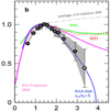 |
Fig. 1. Rotation curve, V/Vmax versus R/R1/2, obtained from a stack of distant galaxies (black dots with error bars) compared to the rotation curve of M31 (red broken line) and the Milky Way (green line) (Fig. 2b of Genzel et al. 2017). |
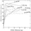 |
Fig. 2. Rotation curves of a sample of nearby galaxies. (Fig. 3 of Rubin et al. 1978). |
The normalisation with respect to size and maximum velocity required to stack the multiple galaxies has been criticised by Tiley et al. (2019), who contends that normalising by the disc radius (Rd) gives different extended rotation curves from normalising by the turnover velocity radius (Rmax), and in fact removes the falling velocities beyond Rmax. However Lang et al. (2018) claims that the fall-off of the rotation curve is independent of the normalisation method, and normalising by R1/2 yields an even more steeply falling rotation curve beyond Rmax.
Genzel et al. (2020) have published a further 41 galaxy rotation curves with redshifts in the range 0.67 < z < 2.45. No stacking of the rotation curves was done and the rotation curves mostly do not extend much beyond Rmax.
For 24 of the galaxies the curve is still rising, having not reached Rmax. For the rest, 8 galaxies have rotation curves which do not decline beyond Rmax, but only 2 of these extend out as far as 2 Rmax, while the remaining 9 that reach Rmax, have sharply declining rotation curves beyond Rmax. Support for the set published in 2017, with stacking out beyond 2 Rmax, is therefore inconclusive.
On the other hand Sharma et al. (2021) have analysed the spectra of 344 galaxy sources in the range 0.57 < z < 1.04 and claim, after correction for kinematic modelling, beam smearing and pressure support from gaseous velocity dispersion, that 256 of their sources have individual flat rotation curves out to a radius of up to 18 kpc, where the median Rd for the sample is ∼3 kpc. One caveat which may serve to differentiate these results from those of Genzel and Lang is that Sharma’s sources have a median z of 0.87, while those of Genzel and Lang have a median z of 1.52, with only a little overlap between the two sets. The lookback time difference between these two median redshifts is almost 2 Gyr which may be significant – see the conclusion section.
This paper presents computer simulations of galaxy formation which show that, irrespective of the initial conditions, if a galaxy forms within a massive dark matter halo then as soon as a stellar disc is formed the gaseous disc will have a non-declining rotation curve to large radius, unlike Fig. 1. So if it turns out that the rotation curves for all distant galaxies are steeply falling, then this implies that galaxies form initially without a massive dark matter halo. But this is contrary to the accepted paradigm for galaxy formation, where the dark matter halo collapses first, followed by the infall of the baryonic matter into the gravitational potential well of the dark matter, where it forms visible stars.
2. Simulations and computational method
The simulations were performed using the code described in Williams & Nelson (2001), Churches et al. (2001, 2004), and Smith et al. (2008, 2010). This code is a standard SPH/Treecode (Monaghan 1992; Barnes & Hut 1986; Hernquist & Katz 1989), employing a 1/(r + ϵ) potential, individual particle timesteps, fully dynamic kernel radius, and star formation via a Schmidt law. The original code assumed an isothermal equation of state, on the basis that any heating of the interstellar gas would be instantly radiated away. However since the velocity dispersion in the interstellar medium has a potentially significant effect on the observed rotation curves, the code was extended to include a full energy equation with cooling and supernova feedback to a turbulent energy component in the dynamic pressure.
The star formation rate was
 (1)
(1)
where ρ is the gas density, ρ⋆ is the star mass density, and k and n are constants. The value 1.25 was used for n, within the range suggested by Kennicutt (1998) based on the gas surface density. If one makes the assumption that a gas disc with a mass of 5 × 10¹⁰ M⊙, a radius of 10 kpc, and a height of 200 pc turns 90% of its mass into stars over a timescale of 5 Gyr with n = 1.25, then the value of k thus obtained is
 (2)
(2)
which was the value used.
The reservoirs of energy in the simulation, apart from the potential and kinetic energy of the dark matter, gas, and eventually star particles, consisted of u, the gas thermal specific energy, and q, the specific energy in turbulent motion created by SN feedback (Springel 2000). These two were governed by the equations
 (3)
(3)
and
 (4)
(4)
Here,
-
v is the gas velocity,
-
Λr is the radiative cooling coefficient = 1.73 × 10²⁰ m5 s−3 kg−1,
-
ΛB is the thermal bremsstrahlung cooling coefficient = 2 × 10¹¹ m4 s−2 kg−1,
-
ΛC is the Compton cooling coefficient = 1.34 × 10⁻²⁰ s−1,
-
Λt is the turbulent decay coefficient = 1.7 × 10⁻¹⁸ m−1,
-
z is the redshift,
-
ΛSN is the supernova heating coefficient = 1.74 × 10¹² m2 s−2,
-
 is the star mass formation rate of Eq. (1),
 -
γ is the ratio of specific heats,
-
T is the temperature = mu/3K where m is a mean atomic mass (equal to 1.4 times the hydrogen atomic mass),
-
K is Boltzmann’s constant,
and
 (5)
(5)
The radiative and Compton cooling formulae were taken from Katz & Gunn (1991), thermal bremsstrahlung (assuming near full ionisation) from Boyd & Sanderson (1969), and the SN feedback formula from Dalla Vecchia & Schaye (2012). The SN feedback method used followed the paradigm outlined by Springel (2000), except that a different formula was used for the decay of turbulent energy to thermal energy, based on the physics of the Kolmogorov cascade, that is dq/dt ∝ −q1.5.
In contrast to the cosmological scale simulations (Schaye et al. 2015; Teklu et al. 2017; Kaviraj et al. 2017; Tremmel et al. 2017; Springel et al. 2018; Dave et al. 2019; Dubois et al. 2021; Bennett & Sijacki 2022), which model large volumes of the early universe leading to multiple galaxy formations, we followed the approach of Katz (1992), and Steinmetz & Muller (1995) which is to model the collapse of isolated spherical perturbations. Although this did not incorporate the interaction of the protogalaxy with nearby intergalactic gas, using ∼100 000 SPH and dark matter particles allows comparable resolution to that of the individual galaxies formed in the cosmological scale simulations. The results presented here focus on the early formation of the gas and stellar discs, and their dynamical properties, which are not greatly affected by interactions with the intergalactic environment.
The purpose of the simulations was to investigate with various initial conditions whether the falling rotation curves reported by Genzel et al. can be replicated within the standard paradigm of a dominant dark matter component. The approach adopted gives more control over the initial conditions of the formation of an individual galaxy than is available in larger scale simulations, while we maintained a strong connection with these simulations by keeping total angular momentum and mass within the expected bounds, and this is reflected in the fact that the resulting dark matter haloes achieve a typical Navarro, Frenk & White (NFW) density profile (see Appendix A).
Various configurations of the initial gas and dark matter spheres were employed, with gas and dark particles set down in uniform density spheres, with positions displaced by small random displacements to emulate Poisson noise. The common feature is that the dark matter component had 83% of the mass, and the baryonic star forming gas eventually fell into the final dark matter potential well. All of the initial scenarios lead to galaxies of similar structure and dynamics, the main reason being that the collapsing protogalaxies went through a violent relaxation phase during which the memory of the detailed initial structure was erased. The amplitude and form of the initial noise in the particle positions also had little effect on the end result, a fact corroborated by Katz & Gunn (1991). Churches (1999) and Churches et al. (2001) also used a range of initial conditions, and showed that the parameters which have the most significant effect on the final galaxy properties are the total mass of the system, and its angular momentum.
The effect of tidal torques by neighbouring gas and dark halos was approximated by setting the initial spheres in solid body rotation. The velocity of rotation was characterised by the dimensionless spin parameter λ given by
 (6)
(6)
where J is the total angular momentum, E is the total energy, M is the total mass of the system, and G is the gravitational constant. The theoretical prediction of Peebles (1971) is that λ is of the order of 0.1, a value that has been confirmed by N body experiments. The initial redshift was set at 100, and the initial ensemble was assumed to have stopped expanding, and started with no radial velocity.
Five different configurations of initial conditions were explored
-
type 1: initial precise coincidence of the gas and dark matter spheres,
-
type 2: the dark matter sphere more collapsed than the gas sphere,
-
type 3: the initial gas and dark matter spheres not coincident,
-
type 4: multiple dark matter spheres embedded in a larger gas sphere,
-
type 5: a gas sphere as in type 1, but no dark matter.
In types 1, 3, and 4 the total mass of the system was 5 × 10¹¹ M⊙, while in type 2 it was 1012 M⊙. In all these types 83% of the initial mass was in dark matter, and 17% in gas. In type 5 the total mass was 8.5 × 10¹⁰ M⊙. The initial radius of the gas sphere in each case was 175 kpc, and in types 2 and 3 a smaller initial radius was used for the dark matter spheres, and a rotational velocity of 0.161 Gyr−1 was applied about the z-axis. This yields in type 1 a total angular momentum of J = 6 × 1067 kg m2 s−1 and a total energy of E = −2 × 1052 J, and thus a spin parameter of 0.13.
The evolution of all of these was followed to the point at which a stable stellar disc was formed with no close mergers, a stellar mass comparable to the gas disc and in the range 2 − 5 × 10¹⁰ M⊙, and with half light radius (R1/2) in or near the range 4–9 kpc (as measured by the stellar number density modified by dust obscuration – see Appendix B). This is the range of R1/2 in the set of galaxies in Fig. 1. The total mass and angular momentum of the systems have been chosen so that the properties of the resulting galaxies at z ∼ 1 matched those of this set.
3. Results
The evolution of each type follows a similar scenario in that the baryonic gas falls into the potential well (or wells) of the collapsing dark matter. This is accompanied by violent relaxation involving strong tidal interactions disrupting and merging sub-galactic clumps, leading to a final relatively smooth and long lived spiral galaxy. The properties of the galaxies at the point where a smooth stellar disc with no merger interactions was established are summarised in Tables 1 and 2. The quantity σ is the total velocity dispersion, incorporating u, q, and the random motion of the SPH particles relative to the bulk motion; and ⟨σ⟩ is the average over radius. Images of the gas, stars and dark matter at this point are displayed in Appendix C, and there are also links in the figure captions to video animations for each of the simulations. In spite of the very different initial configurations of baryonic and dark matter, the violent relaxation intrinsic to the formation process lead to galaxies which are far from being dissimilar. The dark haloes in types 1–4 also relax to an approximate NFW profile by the time the stellar disc is formed (see Appendix A).
3.1. Type 1
This type follows a similar scenario to the phases described in Williams & Nelson (2001): there was (i) an initial collapse to a high density with compression along the z-axis onto the x-y plane, then (ii) re-expansion mainly in the x-y plane, along with fragmentation into massive clumps, (iii) re-collapse accompanied by strong tidal interactions disrupting the sub-galactic clumps, leading to (iv) a long lived spiral galaxy.
A galaxy disc was formed, with 5.2 × 10¹⁰ M⊙ in the stellar disc and 1.75 × 10¹⁰ M⊙ in the gas component, 7.86 Gyr after the start of the simulation. If we take the start of the simulation to have been at a redshift of 100, then this galaxy was formed at z = 0.45. The value of R1/2 was estimated to be between 4.2 and 11.8 kpc, while the radius of the gas disc was estimated to extend out to approximately 70 kpc (see Fig. C.1).
The reason for the wide range in the estimate of R1/2 is because we have taken the obscuration by dust generated during star formation into account, and while we are able to estimate the optical depth of the dust using Churches et al. (2001, 2004), the distribution of gas/dust and stars in the vertical direction was not resolved by the simulations. To calculate the amount of obscuration as a function of radius and hence R1/2, we therefore applied the two extreme cases, (1) dust concentrated in a central layer much smaller than the stellar disc thickness, and (2) dust distributed throughout the stellar disc thickness (see Appendix B). This procedure yielded values of R1/2 equal to 4.2 and 11.8 kpc respectively in the case of type 1, and was applied to all 5 types.
The rotational velocity had a maximum of 211 km s−1. Also in Fig. 3 the velocity dispersion of the gas is plotted as a function of radius. This is a combination of thermal and turbulent velocities derived from the energy equation with input from SN, together with the intrinsic velocity dispersion of the SPH particles arising from the violent relaxation during the galaxy formation process. At this time the average velocity dispersion outside Rmax was 30 km s−1, which was insufficient to add significant support against the dark matter potential well, hence the high rotational velocity.
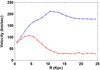 |
Fig. 3. Type 1 rotation curve – rotational velocity (blue) and velocity dispersion (red). |
There are links in the figure captions in Appendix C to videos of all the simulations showing the evolution of the gas, star and dark matter components face-on and edge-on. In the case of type 1 the main stellar disc formed at z = 0.97, but the video in this case runs on to z = 0.45, since there was a significant close satellite of the main galaxy at z = 0.97. The satellite merged with the main galaxy by z = 0.45, at which point we display the rotation curve. In all 5 simulations in this paper we concentrated on the time at which a stable stellar disc had formed, with no significant mergers, though the simulations all ran to much lower redshift with little change in their rotation curves.
3.2. Type 2
This followed a very similar evolution to type 1, except that the dark sphere, which started with a radius of 87 kpc, collapsed and relaxed to a steady configuration more quickly. The gas sphere falls into this deep gravitational well and formed a galaxy disc, with 4.5 × 10¹⁰ M⊙ in the stellar component and 3.3 × 10¹⁰ M⊙ in the gas component, 4.6 Gyr after the start of the simulation. Again this would correspond to a redshift of z = 1.06 if we take the start to be at z = 100. R1/2 is estimated to be between 3.7 and 10.6 kpc, while the radius of the gas disc was estimated to be 50 kpc (see Fig. C.2). Again the rotational velocity was flat out to the outer radius of the gas disc, with a maximum of 225 km s−1 (see Fig. 4, which also shows the gas velocity dispersion). In this case the average velocity dispersion outside Rmax was 37 km s−1.
 |
Fig. 4. Type 2 rotation curve – rotational velocity (blue) and velocity dispersion (red). |
3.3. Type 3
For this simulation the dark matter and gas were two separated spheres each of radius 175 kpc, with their centres separated by 350 kpc, with the dark sphere centred at (x/kpc, y/kpc) = (0, 0), and the gas sphere at (350,0). The dark sphere collapsed as normal to a central relaxed halo, while the gas sphere fell into the potential well of the halo. The gas went through a collapse and re-assemble phase in the centre of the halo, and eventually relaxed to form a galaxy disc, with 2.6 × 10¹⁰ M⊙ in the stellar component and 8.5 × 10¹⁰ M⊙ in the gas component, 5.6 Gyr after the start of the simulation. Again this would correspond to a redshift of z = 0.82 if we assume the start was at z = 100. The value of R1/2 was estimated to be between 3.12 and 12.4 kpc, while the radius of the gas disc was estimated to be 70 kpc (see Fig. C.3). Again the rotational velocity was flat out to the outer radius of the gas disc, with a maximum of 246 km s−1 (see Fig. 5, which also shows the gas velocity dispersion). In this case the average velocity dispersion outside Rmax was 42 km s−1, and the rotation axis was tilted by approximately 5° from the z-axis.
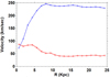 |
Fig. 5. Type 3 rotation curve – rotational velocity (blue) and velocity dispersion (red). |
3.4. Type 4
For this simulation the gas sphere was a uniform density sphere of radius 175 kpc with added noise, while the dark matter mass was split between six smaller spheres of radius 35 kpc, positioned at random within the gas sphere. The dark spheres collapsed as normal, and continued on orbits due to the initial rotational velocity about the centre of the gas sphere. At the same time the gas local to the dark spheres fell into their respective potential wells, and proceeded to form low mass disc galaxies. The dark halos then merged together, as well as their captured gas discs, and formed a more massive halo/galaxy ensemble. The stellar mass of the galaxy disc was 4.3 × 10¹⁰ M⊙ and the gas mass was 3.4 × 10¹⁰ M⊙ at 5.3 Gyr after the start of the simulation, that is at z = 0.89 if we assume the start was at z = 100. The value of R1/2 was estimated to be between 2.6 and 7.5 kpc, while the radius of the gas disc was estimated to be 80 kpc (see Fig. C.4). The rotation axis of this disc galaxy was also no longer along the z-axis, but tilted by 15° to it. After transforming particle positions and velocities, the rotation and dispersion curves of this object are shown in Fig. 6. The maximum rotational velocity was 294 km s−1, and the average velocity dispersion outside Rmax was 44 km s−1.
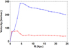 |
Fig. 6. Type 4 rotation curve – rotational velocity (blue) and velocity dispersion (red). |
3.5. Type 5
There may be other initial conditions which would lead to steeply declining rotation curves as in the Genzel result. However it is hard to see how a different configuration of dark matter in relation to the baryons would yield that, given the variety of configurations in types 1–4. The two most important physical quantities which have been found to affect the outcome of the simulations are the mass and angular momentum. Simulations were carried out with less angular momentum than that predicted by Peebles by a factor of 5, but these simply ended with smaller scale galaxies, but with equally high non-declining rotational velocities. The obvious quantity to vary would be the mass of the dark matter. Consequently simulations were carried out with no dark matter, and we present here an example of these. Type 5 has gas only, initially with a mass of 8.5 × 10¹⁰ M⊙ in a sphere of radius 175 kpc, and an initial rotational velocity of 0.0644 Gyr−1. It collapsed under its own gravitational field to form a galaxy disc, with 2 × 10¹⁰ M⊙ in the stellar component and 5.9 × 10¹⁰ M⊙, in the gas component, 5.8 Gyr after the start of the simulation. If we assume a standard ΛCDM cosmology this would correspond to a redshift of z = 0.78 if we take the start to be at z = 100. The value of R1/2 was estimated to be between 3.7 and 16.8 kpc, while the radius of the gas disc was estimated to be 40 kpc (see Fig. C.5). However in this case the rotation curve does decline steeply outside Rmax. The rotation and dispersion curves of this object are shown in Fig. 7, with maximum rotational velocity 195 km s−1 and average velocity dispersion inside a 15 kpc radius of 59 km s−1.
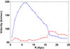 |
Fig. 7. Type 5 rotation curve – rotational velocity (blue) and velocity dispersion (red). |
3.6. Comparison with the Genzel et al. rotation curve
To illustrate the contrast between these results and the rotation curves obtained by Genzel et al. (2017) using stacking, we normalised these rotation curves by Rmax and Vmax and plotted the curves along with the data in Fig. 2b of Genzel et al. (2017) rescaled in radius in Fig. 8.
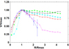 |
Fig. 8. All rotational velocities versus radius, normalised to Rmax and Vmax. Genzel et al. (2017) data – blue hollow circles with error bars, type 1 – red hollow squares, type 2 – black inverted triangles, type 3 – green filled circles, type 4 – turquoise filled squares, type 5 – mauve triangles. |
The rotation curves from types 1–4 are incompatible with the Genzel results. On the contrary type 5 can be seen to give a good match to the Genzel results.
4. Discussion
These simulations demonstrate that if the formation scenario for galaxies is baryonic gas falling into the potential wells of formed, or forming, massive dark matter haloes, then as soon as a stellar disc is formed the gas rotation curve exhibits extended high velocity well beyond Rmax. Figure 8 clearly demonstrates this. The Genzel observations and the results of the simulation types 1–4 are obviously incompatible.
The types 1–4 rotation curves do decline slowly at large radius, but do not descend to half their maximum value until 6–17 Rmax, corresponding to 62–74 kpc. While the Genzel and type 5 rotation curves descend to half-maximum in approximately 2 Rmax, corresponding to 14 kpc in the case of type 5.
A possible explanation for the initial steeply falling rotation curves reported by Genzel et al. could be pressure support by turbulent motion in the interstellar medium. However that would require turbulent velocities ∼100 km s−1, and while, before corrections for beam smearing, the velocity dispersion detected by Genzel et al. has a value of that order at the centre of the galaxies, it quickly drops to ∼50 km s−1 outside Rmax. Similarly low values for intrinsic velocity dispersion, that is 25–50 km s−1 for galaxies ranging from z = 2.3 − 0.9, were obtained by Wisnioski et al. (2015) – see also Ubler et al. (2019).
This is in agreement with the simulations reported here, where the velocity dispersion of the gas has three contributions: deviations from pure rotational motion arising out of violent relaxation, and perturbations due to bar and spiral structures (typically 50–80 km s−1 inside Rmax, but ∼30 km s−1 outside Rmax, at formation of a stellar disc), turbulence from SN feedback (typically ∼30 km s−1 in the central peak but falling to ∼10 km s−1 outside Rmax), and thermal motion (typically ∼10 km s−1 at all radii).
Teklu et al. (2017) have presented cosmological scale galaxy formation simulations in which a subset of galaxies exhibit declining rotation curves similar to the Genzel et al. (2017) results within dark matter haloes, and argue that pressure support by velocity dispersion explains this. Indeed the plot of velocity dispersion which they display for the galaxies which have declining rotation curves (Fig. 4 of their paper) has values ∼100 km s−1 at all radii, which implies that these simulated galaxies do have pressure support from velocity dispersion, unlike the Genzel et al. set. They report that 38% of the galaxies they have studied in detail in their simulation have declining rotation curves, while the other 62% have non-declining rotation curves. The 103 galaxies of the Genzel et al. (2017) set collectively exhibit falling rotation curves, which possibly implies that at high redshift falling rotation curves are universal. If that were the case then significant numbers of flat rotation curve galaxies from cosmological scale galaxy formation simulations such as those of Teklu et al. would be at odds with observations.
Finally, Ubler (2021) have compared the observed kinematic results with the results of the IllustrisTNG cosmological scale simulations, and have concluded that the rotation curves from those simulations imply significantly more dark matter in the simulated galaxies than is indicated by the observations. This supports the conclusion here that the standard galaxy formation scenario within the ΛCDM cosmology, namely that the baryonic gas forming the gaseous and stellar discs collapses by falling into dark matter halos, may be at variance with at least a subset of observations of high redshift galaxy rotation.
5. Conclusion
The evidence to establish that steeply falling rotation curves are universal in galaxies with z ≳ 1 is not yet available. While the sample of galaxies used by Genzel et al. to stack rotation curves, thus extending the rotation curve beyond Rmax, is large, actual measurement of rotational velocity in individual galaxies out to several times Rmax, for a large sample, is required in order to justify such a statement. Recently Puglisi et al (2023) published observations of 22 galaxies with z ∼ 1.5, claiming that they have rotation curves flat out to 6 Rd. However only one of the observed rotation curves extends beyond Rmax; the velocities at 6 Rd were obtained from a modelled extrapolation. To obtain actual measurements of velocity in the outer parts of the high redshift galaxies requires spectroscopy with higher sensitivity and resolution, such as may shortly be obtained using, for instance, the James Webb Space Telescope.
If such observations are obtained, confirming the results of Genzel et al. in a large sample of individual galaxies, then the simulations presented here cast serious doubt on the standard scenario that galaxies form by baryonic gas falling into the potential wells of massive dark matter halos, since the simulations reported here indicate that as soon as a stellar disc is formed, with velocity dispersion ≲50 km s−1, the extended rotation curve under these circumstances will not steeply decline.
The only variation in initial conditions that we could find to reproduce the Genzel results was to remove the dark matter halo in the initial conditions. If no alternative set of initial conditions including a dark halo can be found to reproduce the Genzel results, and they turned out be universal, then this would call into question the very existence of dark matter, since, due to the postulated non-dissipative nature of cold dark matter, it would seem unlikely that dark matter would be captured by a purely baryonic galaxy to produce a flat rotation curve at low z. However that would need to be tested by further simulations.
An alternative explanation for flat rotation curves in galaxies is the modification of distant gravity referred to as MOND – Modified Newtonian Gravity Dynamics Milgrom (1983). However MOND would apply to the high z galaxies as well as contemporary ones, and if the Genzel results are confirmed, then MOND would also be ruled out as well as dark matter haloes.
Another explanation for the flat rotation curves in contemporary galaxies would have to be found, possibly due to the effect of galactic magnetic fields on gas rotation (Nelson 1988; Ruis-Granados et al. 2016). If the steeply falling rotation curves in the range 0.6 < z < 2.6 reported by Genzel et al. (2017), and the flat rotation curves in the range 0.57 < z < 1.04 reported by Sharma et al. (2021) are both confirmed, then one explanation could be that the roughly 2 Gyr interval between the median z of the two respective galaxy sets could be sufficient for the galaxy magnetic field to be generated to a sufficient magnitude to be dynamically significant. The growth time for the magnetic field in a differentially rotating turbulent gas disc is approximately 1–2 Gyr (Panesar & Nelson 1992). However simulations of the generation of galaxy magnetic fields by dynamo action, coupled with the dynamics of MHD, would have to be carried out to establish this explanation.
On the other hand there remains the possibility that some galaxies do form in dark matter haloes, while others do not. The properties of dark matter and baryonic matter are sufficiently different that no satisfactory explanations has so far been put forward as to why they should be locked together in the turbulent primordial universe (Nelson 2022).
Movies
Movie 1 associated with Fig. 4 (xy_xz_full_type4_slow) Access Supplementary Material
Movie 2 associated with Fig. 4 (xy_xz_full_type3_slow) Access Supplementary Material
Movie 3 associated with Fig. 4 (xy_xz_full_type1_slow) Access Supplementary Material
Movie 4 associated with Fig. 4 (xy_xz_centre_type5_slow) Access Supplementary Material
Movie 5 associated with Fig. 4 (xy_xz_centre_type2_slow) Access Supplementary Material
Acknowledgments
We thank an anonymous referee for suggestions to clarify the text.
References
- Barnes, J., & Hut, P. 1986, Nature, 324, 446 [NASA ADS] [CrossRef] [Google Scholar]
- Bennett, J. S., & Sijacki, D. 2022, MNRAS, 514, 313 [CrossRef] [Google Scholar]
- Bosma, A. 1981, AJ, 86, 1825 [NASA ADS] [CrossRef] [Google Scholar]
- Boyd, J. J. M., & Sanderson, J. J. 1969, Plasma Dynamics (London: Thomas Nelson& Sons) [Google Scholar]
- Churches, D. 1999, Ph.D. Thesis, University of Wales, UK [Google Scholar]
- Churches, D., Nelson, A. H., & Edmunds, M. G. 2001, MNRAS, 327, 610 [NASA ADS] [CrossRef] [Google Scholar]
- Churches, D., Nelson, A. H., & Edmunds, M. G. 2004, MNRAS, 347, 1234 [NASA ADS] [CrossRef] [Google Scholar]
- Dalla Vecchia, C., & Schaye, J. 2012, MNRAS, 426, 140 [NASA ADS] [CrossRef] [Google Scholar]
- Dave, R., Anglés-Alcázar, D., Narayanan, D., et al. 2019, MNRAS, 486, 2827 [CrossRef] [Google Scholar]
- de Blok, W. J. G., Walter, F., Brinks, E., et al. 2008, AJ, 136, 2648 [NASA ADS] [CrossRef] [Google Scholar]
- Dubois, Y., Beckmann, R., Bournaud, F., et al. 2021, A&A, 651, 109 [Google Scholar]
- Genzel, R., Forster Schreiber, N. M., Übler, H., et al. 2017, Nature, 543, 397 [NASA ADS] [CrossRef] [Google Scholar]
- Genzel, R., Price, S. H., Übler, H., et al. 2020, ApJ, 902, 98 [NASA ADS] [CrossRef] [Google Scholar]
- Hernquist, L., & Katz, N. 1989, ApJS, 70, 419 [NASA ADS] [CrossRef] [Google Scholar]
- Katz, N. 1992, ApJ, 391, 502 [NASA ADS] [CrossRef] [Google Scholar]
- Katz, N., & Gunn, J. E. 1991, AJ, 377, 365 [NASA ADS] [CrossRef] [Google Scholar]
- Kaviraj, S., Laigle, C., Kimm, T., et al. 2017, MNRAS, 467, 4739 [NASA ADS] [Google Scholar]
- Kennicutt, R. C. J. 1998, ApJ, 498, 541 [NASA ADS] [CrossRef] [Google Scholar]
- Lang, P., Förster Schreiber, N. M., Genzel, R., et al. 2017, ApJ, 840, 92 [NASA ADS] [CrossRef] [Google Scholar]
- Lang, P., Forster Schreiber, N. M., Genzel, R., et al. 2018, https://doi.org/10.5281/zenodo.2595144 [Google Scholar]
- Milgrom, M. 1983, ApJ, 270, 365 [Google Scholar]
- Monaghan, J. J. 1992, ARA&A, 30, 543 [NASA ADS] [CrossRef] [Google Scholar]
- Navarro, J. F., Frenk, C. S., & White, S. D. M. 1996, ApJ, 462, 563 [Google Scholar]
- Nelson, A. H. 1988, MNRAS, 233, 115 [NASA ADS] [Google Scholar]
- Nelson, A. H. 2022, A&A, 661, 84 [Google Scholar]
- Pagel, B. E. J., Simonson, E. A., Terlevich, R. J., & Edmunds, M. G. 1992, MNRAS, 255, 325 [CrossRef] [Google Scholar]
- Panesar, J. S., & Nelson, A. H. 1992, A&A, 264, 77 [NASA ADS] [Google Scholar]
- Peebles, P. J. E. 1971, A&A, 11, 371 [NASA ADS] [Google Scholar]
- Puglisi, A., Dudzeviciute, U., Swinbank, M., et al. 2023, MNRAS, 524, 2814 [NASA ADS] [CrossRef] [Google Scholar]
- Rubin, V. C., & Ford, W. K., Jr. 1970, ApJ, 150, 379 [NASA ADS] [CrossRef] [Google Scholar]
- Rubin, V. C., Ford, W. K., Jr., & Thonnard, N. 1978, ApJ, 225, L107 [NASA ADS] [CrossRef] [Google Scholar]
- Ruis-Granados, B., Battaner, E., & Florido, E. 2016, IAU Symp., 308, 626 [NASA ADS] [Google Scholar]
- Schaye, J., Crain, R. A., Bower, R. G., et al. 2015, MNRAS, 446, 521 [Google Scholar]
- Sharma, G., Salucci, P., Harrison, C. M., et al. 2021, MNRAS, 503, 1753 [CrossRef] [Google Scholar]
- Smith, R., Davies, J. I., & Nelson, A. H. 2008, IAU Symp., 244, 378 [NASA ADS] [Google Scholar]
- Smith, R., Davies, J. I., & Nelson, A. H. 2010, MNRAS, 405, 1723 [NASA ADS] [Google Scholar]
- Sofue, Y., & Rubin, V. C. 2001, ARA&A, 39, 137 [NASA ADS] [CrossRef] [Google Scholar]
- Springel, V. 2000, MNRAS, 312, 859 [NASA ADS] [CrossRef] [Google Scholar]
- Springel, V., Pakmor, R., Pillepich, A., et al. 2018, MNRAS, 475, 676 [Google Scholar]
- Steinmetz, M., & Muller, E. 1995, MNRAS, 276, 549 [NASA ADS] [CrossRef] [Google Scholar]
- Teklu, A. F., Remus, R.-S., Dolag, K., et al. 2017, ApJ, 812, 29 [Google Scholar]
- Tiley, A. L., Swinbank, A. M., Harrison, C. M., et al. 2019, MNRAS, 485, 834 [Google Scholar]
- Tremmel, M., Karcher, M., Governato, F., et al. 2017, MNRAS, 470, 1121 [NASA ADS] [CrossRef] [Google Scholar]
- Ubler, H., Genzel, R., Wisnioski, E., et al. 2019, ApJ, 880, 48 [CrossRef] [Google Scholar]
- Ubler, H., Genel, S., Sternberg, A., et al. 2021, MNRAS, 500, 459 [NASA ADS] [Google Scholar]
- Williams, P. R., & Nelson, A. H. 2001, A&A, 374, 839 [NASA ADS] [CrossRef] [EDP Sciences] [Google Scholar]
- Wisnioski, E., Förster Schreiber, N. M., Wuyts, S., et al. 2015, ApJ, 799, 209 [Google Scholar]
Appendix A: NFW profile fits to the simulation dark matter haloes
The NFW radial density profile (Navarro et al. 1996) is ρNFW(r) = ρ0/ζ(1+ζ)2 where ρ0 is the characteristic density, ζ is r/rs, and rs is the scale radius. Integrating this over the volume of a spherical halo, we obtain for MNFW(r), the total mass inside radius r,
![Mathematical equation: $$ \begin{aligned} M_{\mathrm{NFW}}(r) = 4\pi \rho _{0} r_{s}^{3} \left[ \log (1+\zeta ) - \frac{\zeta }{1+\zeta } \right]. \end{aligned} $$](/articles/aa/full_html/2024/07/aa48833-23/aa48833-23-eq8.gif) (A.1)
(A.1)
Dark matter particles were binned radially in shells such that there were 1000 particles per bin, and the particle masses in each shell summed. The mass profile M(r) was produced by summing shells cumulatively with increasing radius. The NFW mass profile in equation A.1 was then fit to M(r) using a non-linear least-squares algorithm, and ρ0 and rs as fitting parameters. By dividing the mass in each shell by the volume of the shell at r, ρ(r) was computed for the simulation halo. This was plotted along with ρNFW(r) in Fig. A.1.
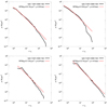 |
Fig. A.1. Simulation halo density profile ρ(r) plotted in black with the corresponding ρNFW(r) in red for each of types 1-4. |
Over most of the radial range there is a remarkably good agreement with the NFW profile in spite of the oblate spheroidal shape of the simulated haloes, and the highly non spherical initial distribution of the dark matter in type 4. This demonstrates the effectiveness of the violent relaxation process in settling the component into a stable configuration. The only significant deviation from the NFW profile occurs at radii > 100 kpc, well outside the galaxy radii, and where the low density of dark material would diminish the integrity of the simulation of the dark component.
Appendix B: Estimation of obscuration
The mass of a star particle in the simulations was 2.5 × 10⁶ M⊙, therefore they represent multiple stars, hence the surface luminosity of the stellar component in the simulations was estimated by simply summing the surface density of star particles. However the simulated galaxies evolved to the point that significant dust would have been ejected into the interstellar medium, sufficient to cause obscuration varying with radius from the centre of the galaxy.
The generation of dust and its obscuring effects was the subject of Churches et al. (2001, 2004), who estimated the generation of heavy elements and the obscuration by dust in the context of simulations of galaxy formation using the same code as in this paper. The optical depth of the galaxy disc is given by equation (7) of Churches et al. (2004)
 (B.1)
(B.1)
where Z is the metallicity, and Ng is the surface number density of gas in m−2. Fig. 2a of Churches et al. (2001) gives the quantity 12+log(O/H) as a function of radius and time, where O/H is the abundance of Oxygen relative to hydrogen. The sloping lines in that figure can be approximated by straight lines with the following equations
 (B.2)
(B.2)
and
 (B.3)
(B.3)
where ts is the time since the start of the simulation.
The values for intermediate times were obtained by interpolation or extrapolation of the straight line coefficients. O/H is related to Z by the approximate equation (Pagel et al. 1992)
 (B.4)
(B.4)
By evaluating the gas surface density in the final frames of each simulation, equations B.1, B.2, B.3, and B.4 were used to evaluate the optical depth of the dust as a function of radius.
However the simulations did not have sufficient resolution in the vertical direction to properly resolve the expected difference of scale height in the gas and stars– the two components have similar rms heights from the simulation. Consequently to calculate the amount of obscuration as a function of radius we used the two extreme cases of (1) dust concentrated in a central layer much smaller than the stellar disc thickness, and (2) dust distributed throughout the stellar disc thickness.
In case 1 the reduction factor of luminosity of the stars by the dust (RF) given optical depth τ, is given by
 (B.5)
(B.5)
while in case 2
 (B.6)
(B.6)
These two cases were applied to the luminosity of the stellar component represented by the surface density of stellar particles, and the resulting distribution was then used to estimate R1/2. The consequent values of R1/2 ranged from 2.6 to 4.2 kpc (average 3.1) over the 5 types in case 1, and 7.5 to 16.8 kpc (average 11.8) in case 2, whereas without taking the dust obscuration into account the range was 1.8 to 3.7 kpc (average 3.0), due to the higher unobscured luminosity at the centre.
Appendix C: Galaxy images
Figs. C.1 to C.5 show images of the surface density for gas, stars, and dark matter at the time in the simulations where the rotation curves were measured, for simulation types 1-5.
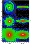 |
Fig. C.1. Type 1 images at z = 0.45. Top to bottom - gas, stars, dark matter; left to right - face-on, edge-on. The size of the panels is 157.5 kpc for gas and stars showing the central regions in more detail, and 350 kpc for dark matter. For an animation of this simulation showing the particle images see https://youtu.be/bRrs5Hu6jYo. The panels in the animation are in the same configuration as this figure, but all with width 350 kpc. Density contours in this figure were rendered logarithmically, from black (< 0.05 M⊙pc−2), blue (∼ 0.5 M⊙pc−2), green (∼ 5 M⊙pc−2), red (∼ 50 M⊙pc−2), to white (> 1000 M⊙pc−2). See online movie. |
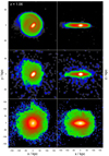 |
Fig. C.2. Type 2 images at z = 1.06. Top to bottom - gas, stars, dark matter; left to right - face-on, edge-on. The size of the panels is 157.5 kpc for gas and stars showing the central regions in more detail, and 350 kpc for dark matter. For an animation of this simulation showing the particle images see https://youtu.be/GGSY-yLBqcg. The panels in the animation are in the same configuration as this figure, but all with width 157.5 kpc. Density contours in this figure were rendered logarithmically, from black (< 0.05 M⊙pc−2), blue (∼ 0.5 M⊙pc−2), green (∼ 5 M⊙pc−2), red (∼ 50 M⊙pc−2), to white (> 1000 M⊙pc−2). See online movie. |
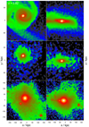 |
Fig. C.3. Type 3 images at z = 0.82. Top to bottom - gas, stars, dark matter; left to right - face-on, edge-on. The size of the panels is 157.5 kpc for gas and stars showing the central regions in more detail, and 350 kpc for dark matter. For an animation of this simulation showing the particle images see https://youtu.be/mtwIU7Qh_g8. The panels in the animation are in the same configuration as this figure, but all with width 157.5 kpc. Density contours in this figure were rendered logarithmically, from black (< 0.05 M⊙pc−2), blue (∼ 0.5 M⊙pc−2), green (∼ 5 M⊙pc−2), red (∼ 50 M⊙pc−2), to white (> 1000 M⊙pc−2). See online movie. |
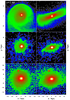 |
Fig. C.4. Type 4 images at z = 0.89. Top to bottom - gas, stars, dark matter; left to right - face-on, edge-on. The size of the panels is 157.5 kpc for gas and stars showing the central regions in more detail, and 350 kpc for dark matter. For an animation of this simulation showing the particle images see https://youtu.be/3j2rUXx7NOQ. The panels in the animation are in the same configuration as this figure, but all with width 350 kpc. Density contours in this figure were rendered logarithmically, from black (< 0.05 M⊙pc−2), blue (∼ 0.5 M⊙pc−2), green (∼ 5 M⊙pc−2), red (∼ 50 M⊙pc−2), to white (> 1000 M⊙pc−2). See online movie. |
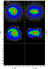 |
Fig. C.5. Type 5 images at z = 0.78. Top to bottom - gas, stars; left to right - face-on, edge-on. The size of the panels is 157.5 kpc for gas and stars showing the central regions in more detail. (Note that there was no dark matter component included in this simulation.) For an animation of this simulation showing the particle images see https://youtu.be/NCnqIOLRyDg. The panels in the animation are in the same configuration as this figure, and also have a width of 157.5 kpc. Density contours in this figure were rendered logarithmically, from black (< 0.05 M⊙pc−2), blue (∼ 0.5 M⊙pc−2), green (∼ 5 M⊙pc−2), red (∼ 50 M⊙pc−2), to white (> 1000 M⊙pc−2). See online movie. |
All Tables
All Figures
|
Fig. 1. Rotation curve, V/Vmax versus R/R1/2, obtained from a stack of distant galaxies (black dots with error bars) compared to the rotation curve of M31 (red broken line) and the Milky Way (green line) (Fig. 2b of Genzel et al. 2017). |
| In the text | |
|
Fig. 2. Rotation curves of a sample of nearby galaxies. (Fig. 3 of Rubin et al. 1978). |
| In the text | |
|
Fig. 3. Type 1 rotation curve – rotational velocity (blue) and velocity dispersion (red). |
| In the text | |
|
Fig. 4. Type 2 rotation curve – rotational velocity (blue) and velocity dispersion (red). |
| In the text | |
|
Fig. 5. Type 3 rotation curve – rotational velocity (blue) and velocity dispersion (red). |
| In the text | |
|
Fig. 6. Type 4 rotation curve – rotational velocity (blue) and velocity dispersion (red). |
| In the text | |
|
Fig. 7. Type 5 rotation curve – rotational velocity (blue) and velocity dispersion (red). |
| In the text | |
|
Fig. 8. All rotational velocities versus radius, normalised to Rmax and Vmax. Genzel et al. (2017) data – blue hollow circles with error bars, type 1 – red hollow squares, type 2 – black inverted triangles, type 3 – green filled circles, type 4 – turquoise filled squares, type 5 – mauve triangles. |
| In the text | |
|
Fig. A.1. Simulation halo density profile ρ(r) plotted in black with the corresponding ρNFW(r) in red for each of types 1-4. |
| In the text | |
|
Fig. C.1. Type 1 images at z = 0.45. Top to bottom - gas, stars, dark matter; left to right - face-on, edge-on. The size of the panels is 157.5 kpc for gas and stars showing the central regions in more detail, and 350 kpc for dark matter. For an animation of this simulation showing the particle images see https://youtu.be/bRrs5Hu6jYo. The panels in the animation are in the same configuration as this figure, but all with width 350 kpc. Density contours in this figure were rendered logarithmically, from black (< 0.05 M⊙pc−2), blue (∼ 0.5 M⊙pc−2), green (∼ 5 M⊙pc−2), red (∼ 50 M⊙pc−2), to white (> 1000 M⊙pc−2). See online movie. |
| In the text | |
|
Fig. C.2. Type 2 images at z = 1.06. Top to bottom - gas, stars, dark matter; left to right - face-on, edge-on. The size of the panels is 157.5 kpc for gas and stars showing the central regions in more detail, and 350 kpc for dark matter. For an animation of this simulation showing the particle images see https://youtu.be/GGSY-yLBqcg. The panels in the animation are in the same configuration as this figure, but all with width 157.5 kpc. Density contours in this figure were rendered logarithmically, from black (< 0.05 M⊙pc−2), blue (∼ 0.5 M⊙pc−2), green (∼ 5 M⊙pc−2), red (∼ 50 M⊙pc−2), to white (> 1000 M⊙pc−2). See online movie. |
| In the text | |
|
Fig. C.3. Type 3 images at z = 0.82. Top to bottom - gas, stars, dark matter; left to right - face-on, edge-on. The size of the panels is 157.5 kpc for gas and stars showing the central regions in more detail, and 350 kpc for dark matter. For an animation of this simulation showing the particle images see https://youtu.be/mtwIU7Qh_g8. The panels in the animation are in the same configuration as this figure, but all with width 157.5 kpc. Density contours in this figure were rendered logarithmically, from black (< 0.05 M⊙pc−2), blue (∼ 0.5 M⊙pc−2), green (∼ 5 M⊙pc−2), red (∼ 50 M⊙pc−2), to white (> 1000 M⊙pc−2). See online movie. |
| In the text | |
|
Fig. C.4. Type 4 images at z = 0.89. Top to bottom - gas, stars, dark matter; left to right - face-on, edge-on. The size of the panels is 157.5 kpc for gas and stars showing the central regions in more detail, and 350 kpc for dark matter. For an animation of this simulation showing the particle images see https://youtu.be/3j2rUXx7NOQ. The panels in the animation are in the same configuration as this figure, but all with width 350 kpc. Density contours in this figure were rendered logarithmically, from black (< 0.05 M⊙pc−2), blue (∼ 0.5 M⊙pc−2), green (∼ 5 M⊙pc−2), red (∼ 50 M⊙pc−2), to white (> 1000 M⊙pc−2). See online movie. |
| In the text | |
|
Fig. C.5. Type 5 images at z = 0.78. Top to bottom - gas, stars; left to right - face-on, edge-on. The size of the panels is 157.5 kpc for gas and stars showing the central regions in more detail. (Note that there was no dark matter component included in this simulation.) For an animation of this simulation showing the particle images see https://youtu.be/NCnqIOLRyDg. The panels in the animation are in the same configuration as this figure, and also have a width of 157.5 kpc. Density contours in this figure were rendered logarithmically, from black (< 0.05 M⊙pc−2), blue (∼ 0.5 M⊙pc−2), green (∼ 5 M⊙pc−2), red (∼ 50 M⊙pc−2), to white (> 1000 M⊙pc−2). See online movie. |
| In the text | |
Current usage metrics show cumulative count of Article Views (full-text article views including HTML views, PDF and ePub downloads, according to the available data) and Abstracts Views on Vision4Press platform.
Data correspond to usage on the plateform after 2015. The current usage metrics is available 48-96 hours after online publication and is updated daily on week days.
Initial download of the metrics may take a while.