| Issue |
A&A
Volume 686, June 2024
|
|
|---|---|---|
| Article Number | A240 | |
| Number of page(s) | 12 | |
| Section | Astronomical instrumentation | |
| DOI | https://doi.org/10.1051/0004-6361/202449589 | |
| Published online | 18 June 2024 | |
A new approach for the numerical calculation of diffraction patterns using starshades
Université Côte d’Azur, Observatoire de la Côte d’Azur, CNRS, parc Valrose,
06108
Nice,
France
e-mail: This email address is being protected from spambots. You need JavaScript enabled to view it.
Received:
13
February
2024
Accepted:
25
March
2024
Abstract
Context. We studied the imaging of exoplanetary systems using starshades, which are externally occulted coronagraphs in space.
Aims. We provide a new method for precisely evaluating the stray light due to the star and a rapid calculation of the point spread functions in the presence of vignetting effects from the external occulter. Our study used shaped occulter configurations published in the literature, in particular, the SISTER NI2 and NW2 systems.
Methods. The wavefront at the telescope aperture was computed using the classic Fresnel filtering method. The Fourier transform of the occulter was obtained with the highest possible precision using an approach initially developed for radio antennas, known as the polygonal shape factor.
Results. We show that the Fresnel diffraction for a finite spatial field operates at very low frequencies only, and that it is sufficient to calculate the Fourier transforms there. Diffraction patterns computed numerically fully agree with theoretical predictions. The central parts of diffractions of petal and apodized occulters are identical over a large central area that increases in size with the number of petals. These diffraction patterns are used to compute the point spread functions. We computed the stray light for a non-point source star; this shows that starshades are not sensitive to star leakage, with a star diameter limit for a given configuration. We also computed signal-to-noise ratios for a perfect experiment limited by photon noise.
Key words: instrumentation: high angular resolution / methods: numerical / techniques: high angular resolution
© The Authors 2024
 Open Access article, published by EDP Sciences, under the terms of the Creative Commons Attribution License (https://creativecommons.org/licenses/by/4.0), which permits unrestricted use, distribution, and reproduction in any medium, provided the original work is properly cited.
This article is published in open access under the Subscribe to Open model. This email address is being protected from spambots. You need JavaScript enabled to view it. to support open access publication.
1 Introduction
Starshades are space-based experiments for exoplanet imaging. They require two spacecraft, the first bearing the occulter and the second the observing telescope. Ideally, the occulter blocks all the starlight and allows one to see faint exoplanets that are outside the inner working angle (IWA) of the occulter. The occulter is fully opaque and has a petal shape to achieve the darkest shadow possible (Cash 2006; Vanderbei et al. 2007; Arenberg et al. 2021).
The first experiments with an external occulter were developed for the solar corona. The precursor was the visual sky photometer of Evans (1948). Almost all solar-space experiments used an external occulter coupled with a Lyot (1933) corona-graph. As described by Koutchmy (1988), a single spacecraft was used, with the occulter held in front of the telescope by a metal arm. Occulters of various shapes – including serrated occulters, a forerunner of the petal occulter with triangular teeth instead of petals of a very studied shape – or multiple disk occulters were used (Tousey 1965; Koomen et al. 1975; Newkirk & Bohlin 1965; Brueckner et al. 1995). The solar coronagraph ASPIICS (Association of Spacecraft for Polarimetric and Imaging Investigation of the Corona of the Sun) (Lamy et al. 2010; Renotte et al. 2014), which is expected to fly very soon, will be the first-ever formation-flying two-spacecraft coronagraph and could serve as a real small-size test for starshades.
Although solar and stellar coronagraphs with an external occulter share similar concepts, their geometrical dimensions differ significantly. The so-called “giant” ASPIICS solar coronagraph is a R = 0.71 m radius circular occulter, positioned at Z = 144 m in front of a D = 5 cm diameter aperture Lyot's coronagraph. The Fresnel number, Φ = R2/(λZ), is on the order of 7000 at λ = 500 nm, and the angle obscured by the occulter, R/Z, is very large, on the order of 0.005 rd, because of the solar disk. The numerical analysis made by Rougeot et al. (2017) proved the efficiency of combining external occultation with an internally occulted Lyot-style coronagraph.
For exoplanets, the values are completely different (Cash 2006). For example, the SISTER (Starshade Imaging SimulationToolkit for Exoplanet Reconnaissance)1 configuration NI2 (Hildebrandt et al. 2021) is a petal-shaped occulter of radius R = 13 m at Z = 37 342 km. The Φ value at a wavelength of 500 nm is approximately 9, and the geometrical IWA (R/Z) is about 3.5 × 10⁻⁷ rd, or 72 mas (milliarcsec). For the NW2 configuration – an occulter of R = 36 m at Z = 119 770 km − φ ~ 21.6, and the IWA is about 3.0 × 10⁻⁷ rd, or 62 mas.
The computation of the Fresnel diffraction for a petal-shaped occulter is a difficult problem of precision, as described in the literature. Barnett (2021) used a technique of areal quadrature, while Cady (2012) and Harness et al. (2018) used the Maggi--Rubinowicz representation approach (Born & Wolf 2013). Instead of the 2D integral of the Fresnel formulation, this method relies on a single boundary integral along the edge of the diffracting object. This was also the approach of Rougeot & Aime (2018) for the serrated occulter.
Another method, which relies on the 2D convolution integral of the Fresnel formulation, is used in this paper: it is based on a polygonal approximation of the petal-shaped occulter boundary. Efficient numerical methods for computing the (continuous) Fourier transform are available (Lee & Mittra 1983; Wuttke 2021), alleviating the problems of aliasing that otherwise plague the Fourier transform computation of a binary occulter transmission function.
The paper is organized as follows. Section 2 presents a new approach to numerically calculating the diffracted wave at the telescope level. We show that Fresnel filtering for a bounded field is a very low-frequency filtering. We also describe the numerical implementation of the Fourier transform of the occulter's indicator function. In Sec. 3, we show that the numerical calculations are in full agreement with the Vanderbei et al. (2007) theoretical predictions. Section 4 gives examples of residual stray light for a non-point source star, point spread function (PSF) patterns, and estimations of the signal-to-noise ratio (S/N). Conclusions are given in Sect. 5, and two appendices detail certain points of the calculations.
2 Calculation of the wavefront on the telescope
2.1 Some useful properties of the Fresnel diffraction
Fresnel diffraction is a classic problem that has been treated in many textbooks, including Born & Wolf (2013) and Goodman (1968). For an occulting mask of f(r), r = (x, y), it is useful to write the transmission of the numerical calculation of the Fresnel diffraction in the complementary form:
![Mathematical equation: $\[f(\boldsymbol{r})=1-t(\boldsymbol{r}),\]$](/articles/aa/full_html/2024/06/aa49589-24/aa49589-24-eq1.png) (1)
(1)
where t(r) corresponds to a transparent mask that is spatially bounded, so t(r) = 0 for ∥r∥ > R.
Let Ψλ(ξ r, Z) be the wave diffracted at distance z = Z by an occulter located at z = 0 in response to an incident plane wave coming from the direction ξ = (ξx, ξy). For ξ = 0, we have
![Mathematical equation: $\[\begin{aligned}\Psi_\lambda(\mathbf{0}, \boldsymbol{r}, Z) & =f(\boldsymbol{r}) * \frac{1}{i \lambda Z} \exp \left(i \pi \frac{\|\boldsymbol{r}\|^2}{\lambda Z}\right) \\& =1-t(\boldsymbol{r}) * \frac{1}{i \lambda Z} \exp \left(i \pi \frac{\|\boldsymbol{r}\|^2}{\lambda Z}\right),\end{aligned}\]$](/articles/aa/full_html/2024/06/aa49589-24/aa49589-24-eq2.png) (2)
(2)
where we have used the property that an infinite plane wave propagates as an infinite plane wave, which is a trivial solution of the wave equation, or alternatively that the infinite integral of the quadratic phase equals 1 (e.g., the convolution with 1 is 1). This property is very often referred to as Babinet's theorem (Vanderbei et al. 2007; Cady 2012).
For an angle ξ ≠ 0, it is easy to show that
![Mathematical equation: $\[\Psi_\lambda(\boldsymbol{\xi}, \boldsymbol{r}, Z)=\Psi_\lambda(0, \boldsymbol{r}+\boldsymbol{\xi} Z, Z) \exp \left(-2 i \pi \frac{\boldsymbol{r} \boldsymbol{.\xi}}{\lambda}\right)\]$](/articles/aa/full_html/2024/06/aa49589-24/aa49589-24-eq3.png) (3)
(3)
where r.ξ = xξx + yξy. This equation shows that it suffices to calculate the Fresnel diffraction, Ψλ(0, r, Z), for a single wave corresponding to rays parallel to the axis (see, e.g., Aime 2013 for a demonstration of this property).
Another interesting property is the similarity relation of the Fresnel diffraction. Two screens – f(r) and f(r/a), which differ in size only – present similar Fresnel diffraction patterns, ϕ(r) and ϕ(r/a), if observed at distances Z and a2Z, respectively. This result is well known and arises from the fact that such configurations have the same Fresnel number. Thanks to geometric optics, this preserves the étendue of the beam. The IWA (R/Z, where R is the radius of the occulter) shrinks as the size of the system grows.
For example, we considered the NW2 configuration from the SISTER project (Hildebrandt et al. 2021), which gives extinctions below 10−10 for a 4 m telescope. Its parameters are an occulter radius, R, of 36 m and a distance Z = 1.1977 × 10⁸ m. The IWA is roughly 3.0058 × 10⁻⁷ rd, or 62 mas (milliarcsecond). The same 10−10 performance for the 6.5 m JWST, whose diameter is as large (a = 1.625), would be obtained using an occulter of the same shape enlarged to 117 m in diameter and set at the distance Z = 3.1626 × 10⁸ m. The IWA would then be reduced to 1.8497 × 10⁻⁷ rd, or 38 mas.
2.2 Numerical aspects
For an opaque mask, the diffraction pattern can be obtained from a curvilinear integral carried out along the edges of the diffracting object. This boundary diffraction approach was first invented by Maggi and later by Rubinowicz more than a century ago. It can be derived from Kirchhoff's integral theorem (Born & Wolf 2013). It has been extensively used for Fresnel diffraction calculations for starshade (Hildebrandt et al. 2021) and for the diffraction of a serrated occulter in solar coronagraphy (Rougeot & Aime 2018).
In the present study, we used the classical Fresnel filtering approach, which makes it possible to easily compare shaped and apodized occulters. The calculation of Eq. (2) can be done directly by convolution, but this operation is very slow and it is generally preferable to go back and forth in the Fourier space:
![Mathematical equation: $\[\Psi_\lambda(\mathbf{0}, \boldsymbol{r}, Z)=1-\mathcal{F}^{-1}\left[\hat{t}(\boldsymbol{\rho}) \times \mathcal{F}\left[\frac{1}{i \lambda Z} ~\exp \left(i \pi \frac{\|\boldsymbol{r}\|^2}{\lambda Z}\right)\right]\right],\]$](/articles/aa/full_html/2024/06/aa49589-24/aa49589-24-eq4.png) (4)
(4)
where ![Mathematical equation: $\[\mathcal{F}[] \text { and } \mathcal{F}^{-1}[]\]$](/articles/aa/full_html/2024/06/aa49589-24/aa49589-24-eq5.png) stand for the 2D direct and inverse Fourier transforms and
stand for the 2D direct and inverse Fourier transforms and ![Mathematical equation: $\hat{t}(\bm{\rho})=\mathcal{F}[t(\bm{r}) ]$](/articles/aa/full_html/2024/06/aa49589-24/aa49589-24-eq6.png) , with ρ = (u, υ) the vector of spatial frequencies. We note that the effect of the wavelength, λ, is given by the Fourier transform of the quadratic phase term.
, with ρ = (u, υ) the vector of spatial frequencies. We note that the effect of the wavelength, λ, is given by the Fourier transform of the quadratic phase term.
In the Fresnel filtering approach, a classic problem is sampling the kernel versus the diffracting object, as discussed by Mas et al. (2003). Here, we present a new approach to this old problem: we considered a finite-dimension object and its finite diffraction pattern. Our results are surprising and counterintuitive. The Fresnel filter appears as a very low pass filter, therefore not requiring very tight sampling. Consequently, only the low frequencies of the Fourier transform of the occulter will be concerned. Nevertheless, because the shaped occulter is a discontinuous function at the occulter boundary, its Fourier transform amplitude decreases very slowly with wave number, and a very tight sampling of the occulter would remain mandatory to avoid aliasing issues in the convolution integral if one uses a discrete (pixelized) description of the occulter.
We instead used a polygonal approximation of the occulter, which allows an accurate, aliasing-free computation of its (continuous) Fourier transform at arbitrary positions in the uυ plane. Details of this method are given in Sect. 2.2.2.
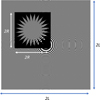 |
Fig. 1 Illustration of the convolution in Eq. (2) where the transparent occulter t(r) from Eq. (1) of size 2R × 2R sweeps the quadratic phase (real part here) shown for a region 2L × 2L. The occulter corresponds to the NI2 configuration. Because of edge effects, the convolution is obtained in the region limited to 2(L − R) × 2(L − R). |
2.2.1 Sampling the Fresnel filter
The Fourier transform of the quadratic phase term is known as the Fresnel filter, which admits an analytic form:
![Mathematical equation: $\[\mathcal{F}\left[\frac{1}{i \lambda Z} \exp \left(i \pi \frac{\|\boldsymbol{r}\|^2}{\lambda Z}\right)\right]=\exp \left(-i \pi \lambda z\|\boldsymbol{\rho}\|^2\right).\]$](/articles/aa/full_html/2024/06/aa49589-24/aa49589-24-eq7.png) (5)
(5)
This complex function takes the form of a 2D chirp and oscillates very fast as the frequency increases. This becomes a very severe sampling problem for large ∥ρ∥2 = u2 + υ2 values. This has led to stringent sampling conditions for solar coronagraphy (Rougeot & Aime 2018) that uses external serrated occulters.
The problem arises when one uses exp(−iπλz∥ρ∥2) directly in Eq. (4). This ideal quadratic phase of Eq. (5) corresponds to an infinite integral only. We can consider that the sampled field is limited in x and y from −L to +L (i.e., over a square of dimensions 2L × 2L). An illustration of the convolution of an occulter t(r) with the quadratic phase is given in Fig. 1.
We demonstrate in Appendix A that in this case the Fourier transform is restricted to low frequencies by functions FL(u) and FL(υ). Rewriting Eq. (5) in x, y, u, and υ, we have
![Mathematical equation: $\[\begin{aligned}{r}\mathcal{F}\left[\frac{1}{i \lambda Z} \exp \left(i \pi \frac{x^2+y^2}{\lambda Z}\right) \Pi\left(\frac{x}{2 L}\right) \Pi\left(\frac{y}{2 L}\right)\right]\\=\exp \left(-\mathrm{i} \pi \lambda z\left(u^2+v^2\right)\right) F_L(u) F_L(v).\end{aligned}\]$](/articles/aa/full_html/2024/06/aa49589-24/aa49589-24-eq8.png) (6)
(6)
The function FL(ρ) = FL(u)FL(υ) acts as a low-pass filter that confines the Fresnel filter exp(−iπλz∥ρ∥2) of Eq. (5) mainly to low frequencies. The low freqencies tend to vanish for |u| and |υ| values that are greater than the value uL:
![Mathematical equation: $\[u_{\mathrm{L}}=\frac{L}{\lambda Z}.\]$](/articles/aa/full_html/2024/06/aa49589-24/aa49589-24-eq9.png) (7)
(7)
The uL can be converted to a number of significant frequency points, nL by dividing it by the spectral resolution 1/2L:
![Mathematical equation: $\[n_{\mathrm{L}}=\frac{L / \lambda Z}{1 / 2 L}=2 \frac{L^2}{\lambda Z}=2 \Phi^{\prime} \text {, }\]$](/articles/aa/full_html/2024/06/aa49589-24/aa49589-24-eq10.png) (8)
(8)
where Φ′ is the Fresnel number associated with the entire field in which the diffraction is computed. For exoplanets experiments, nL will be on the order of a few hundred to a few thousand, while it becomes extremely high for the solar case.
2.2.2 Numerical implementation of ![Mathematical equation: $\[\hat{t}(\boldsymbol{\rho})\]$](/articles/aa/full_html/2024/06/aa49589-24/aa49589-24-eq11.png)
Despite the fact that the Fresnel convolution integral on a field of a finite extent limits, in practice, the Fourier amplitude of the Fresnel filter to relatively low angular frequencies, great care must be taken to control the aliasing power in the computation of the Fourier transform of the discontinuous occulter transmission. In the context of radio antenna computations (secondary patterns, frequency-selective surfaces, etc.), Lee & Mittra (1983) derived a closed-form formula for a polygonal shape factor (the continuous Fourier transform of the indicator function of the surface delimited by a polygon) in terms of a sum over the polygon vertices, with geometric and complex exponential factors. This formula was later re-derived and improved upon by Wuttke (2021) to obtain a numerically stable form for small wave numbers, without undefined values on the u = 0 and υ = 0 axes of the uv plane. The method presented here is based on the Wuttke (2021) version, and we closely follow their notations.
We assumed that we can appropriately describe the boundary region of the petal occulter as a polygon, with vertices coordinates {vj = j = 1 ... N}, so t(r) = 1 within this polygon and 0 outside. Obviously, points at the tip and at the base of the petals should be included in the vertices, and an increasing number of vertices should allow a more accurate description of the occulters.
Wuttke (2021) shows that the continuous Fourier transform t(r), namely ![Mathematical equation: $\[\hat{t}(\boldsymbol{\rho})\]$](/articles/aa/full_html/2024/06/aa49589-24/aa49589-24-eq12.png) , can be computed as
, can be computed as
![Mathematical equation: $\[\hat{t}(\boldsymbol{\rho})=\frac{1}{i \pi\|\boldsymbol{\rho}\|^2} ~\sum_{j=1}^N\left[\hat{\mathbf{n}}, \boldsymbol{\rho}, \mathbf{e}_j\right]\left(\operatorname{sinc}\left(2 \pi \boldsymbol{\rho} \boldsymbol{.e}_j\right) e^{i 2 \pi \boldsymbol{\rho.r}_j}-c\right),\]$](/articles/aa/full_html/2024/06/aa49589-24/aa49589-24-eq13.png) (9)
(9)
where ![Mathematical equation: $\[\hat{\mathbf{n}}\]$](/articles/aa/full_html/2024/06/aa49589-24/aa49589-24-eq14.png) is the unit vector normal to the plane of the polygon, [a, b, c] = det [a, b, c] is the vector triple product, and c is an arbitrary constant that can be chosen to alleviate numerical errors in the small ∥ρ∥ limit. Finally, ej = (vj+1 − vj)/2 and rj = (vj+1 + vj)/2. The derivation of Eq. (9) is given in Appendix B.
is the unit vector normal to the plane of the polygon, [a, b, c] = det [a, b, c] is the vector triple product, and c is an arbitrary constant that can be chosen to alleviate numerical errors in the small ∥ρ∥ limit. Finally, ej = (vj+1 − vj)/2 and rj = (vj+1 + vj)/2. The derivation of Eq. (9) is given in Appendix B.
For large values of ∥ρ∥, c = 0 is the best choice to avoid roundoff errors in the numerator, while for small values of ∥ρ∥, choosing c = 1 removes factors in 1/∥ρ∥ × Σj ej (see Eq. (B.3)); in principle, these terms do not contribute as this sum in Eq. (9) is null (the polygon is a closed shape), but any numerical error on that sum can be amplified by the factor 1/∥ρ∥ if c is not chosen carefully in the small ∥ρ∥ regime. Another way to get rid of these numerical issues is to consider the case of a polygon with a central symmetry; assuming for simplicity that the center of symmetry is the origin of the coordinates (which can always be assumed), the Fourier transform formula becomes
![Mathematical equation: $\[\hat{t}(\boldsymbol{\rho})=\frac{2}{i \pi\|\boldsymbol{\rho}\|^2} \sum_{j=1}^{N / 2}\left[\hat{\mathbf{n}}, \boldsymbol{\rho}, \mathbf{e}_j\right] \operatorname{sinc}\left(2 \pi \boldsymbol{\rho} \boldsymbol{.e}_j\right) \operatorname{sinc}\left(2 \pi \boldsymbol{\rho}\boldsymbol{.r}_j\right).\]$](/articles/aa/full_html/2024/06/aa49589-24/aa49589-24-eq15.png) (10)
(10)
In this case there is no term proportional to 1/∥ρ∥, and this formula is numerically stable for all values of ∥ρ∥. It can therefore be used as is in the case of the petal occulter, which has a central symmetry. The wavefront is finally obtained by applying an inverse 2D Fourier transformation according to Eq. (4).
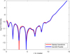 |
Fig. 2 Comparison between cuts of the intensity diffraction pattern for the apodized occulter of the NW2 configuration at 500 nm (central shadow, log10 scale). The red curve, computed using a Hankel transform, is almost identical to the blue curve, which is a radial cut of the pattern obtained using 2D Fourier transforms. |
3 Comparing Fresnel diffractions of petal and apodized occulters at the telescope aperture plane
For an occulter of variable transmission, its Fourier transform is done classically using a fast Fourier transform algorithm that can be implemented in two times, first the transform of x into u using n points on a line as input and only m points as output for the transform, followed by a transform of y into υ. Due to the low value of nL, this allows one to reduce the memory requirement of the computer; the largest array is only n × m. The result is m × m; the m should be somewhat greater than nL to ensure a good sampling of the wave on the telescope aperture and the final calculation of the PSF. In the present study we used m = 8192. Alternatively, since the apodized occulter has a symmetry of revolution, we could use a Hankel transform. A comparison between the two computations is shown in Fig. 2.
An example of intensities of Fresnel diffraction patterns produced by an apodized occulter and a petal occulter at the telescope aperture plane is given in Fig. 3 on a linear scale. The occulter is the one shown in Fig. 1 for the SISTER configuration NI2 (Hildebrandt et al. 2021). It is a 24-petal shaped occulter of radius R = 13 m at Z = 37 342 km, and the Fresnel diffraction was calculated for λ = 500 nm. The 2D intensity figures clearly show the strong differences between the smooth diffraction pattern of the apodized occulter and the structured one of the petal occulter. This difference is quantitatively more visible when the radial cuts are compared; these cuts are drawn here for two locations, corresponding to a tip of a petal (θ = 0) and a hollow between two petals (θ = &pi:/24). Intensity fluctuations are significant in the vignetting region of the telescope, which corresponds to the projected position of the petals of the occulter.
Figure 4 gives an illustration of the variation in the diffraction pattern with the wavelength in the vignetting zone. To facilitate the comparison, we considered the same angular portion of π/12 (from tip to tip of the petals) of the diffraction pattern, which we have represented in polar coordinates as a rectangle for the seven wavelengths considered in SISTER for NI2, for example 425-552 nm. The structures deform and move toward larger ∥r∥ with larger λ.
Figure 5 gives an example of what can be obtained for the dark central part of the diffraction pattern (modulus and phase) of apodized and petal occulters for the NW2 SISTER configuration. In the central region, the diffraction pattern of the petal occulter loses its periodic variable structure and tends to become very similar to the diffraction of the apodized occulter, up to a radius of about 4 m (the red circle).
This behavior is fairly well predicted by the theoretical approach of Vanderbei et al. (2007). We illustrate this in Fig. 6. The top panel gives cuts of the numerical intensities shown in Fig. 5 and the bottom panel the results obtained using Eq. (9) from Vanderbei et al. (2007). In their model, the apodized diffraction pattern, which can be written as a Hankel transform of the apodization profile, is the first term of an infinite series that describes the petal diffraction pattern (curves in blue). Successive terms of the series involve Bessel functions whose order grows in proportion to the number of petals. The small residual differences that appear in the central cuts between apodized and petal occulters (top panel of Fig. 6) might be attributed to the difficulty in calculating the diffraction pattern of the petal occulter.
Using fewer or more petals will modify the size of regions where the apodized and petal occulters are similar. Figure 7, also drawn using the Vanderbei et al. (2007) model, illustrates the influence of the number of petals for the NW2 and NI2 configurations. Using more petals with NW2, for example 36 petals instead of 24, can enlarge the central dark zone. To the contrary, NI2 can use fewer petals, for example 16 petals instead of 24, to form the same central dark area.
The conclusion that can be drawn from these two examples is that it is enough to compute the Fresnel diffraction of the apodized occulter to estimate the dark central zone with high accuracy. Beyond this central zone, as soon as we approach the geometric edges of the occulter, the diffraction pattern does not require very high calculation precision, and a simple calculation using Fresnel filtering and a few thousand points is enough.
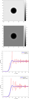 |
Fig. 3 Intensity diffraction pattern (linear scale) for the NI2 configuration at λ = 500 nm. Top panels: 2D representations of a zone of 80 × 80 m for the apodized occulter (top panel) and the petal occulter (second panel). Bottom two panels: radial cuts for the angles θ = 0 and θ = π/24. The strong variations for the petal occulter contrast with the smooth variations for the apodized occulter. |
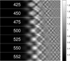 |
Fig. 4 Variation with λ from 425 to 552 nm of a periodic angular sector anamorphosed to a rectangle in the coordinates ∥r∥ × θ, ∥r∥ from 0 to 23 m, θ from 0 to π/12, and corresponding to the periodicity of the 24-petal occulter. |
4 Residual stray light, PSF patterns, and global characteristics
The response of the telescope to a point source at infinity is obtained by taking the modulus squared of the Fourier transform of the wave it produces on the telescope aperture. PSF responses are obtained by sweeping the wavefront – Ψλ(ξ, r, Z) of Eq. (3) – across the aperture for the corresponding angular directions of observation. We used the wavefront of the apodized occulter to determine the stray light due to the star and the wavefront of the petal occulter to derive the variable PSFs (see Sect. 3).
The residual light from the star was obtained by considering an on-axis point source. In this case the telescope receives the central part of the wave, which, as we recall, is the same for the apodized occulter and the petal occulter. For a star whose apparent diameter is not zero, we had to add up all the contributions from the star's disk by moving the wavefront by the desired amount and applying the corresponding tilt. In Fig. 8, we show a result for a point source star and for a star with an angular diameter of 1.5 mas. For this illustration, we calculated the responses corresponding to 481 points of uniform intensity on the stellar disk, ignoring any possible center-to-edge variation, a variation that could easily be introduced. The telescope we used was 4 m with a central obstruction.
The difference between curves for a point source or finite diameter star is visible but is not really significant, and we conclude that a starshade system is rather insensitive to star leakage as long as the diameter of the star does not cause a displacement of the shadow greater than the central dark zone of the occulter. For the NW2 system, 1 mas corresponds to a displacement of 0.58 m, which would mean that a star of 13 mas would be a limit, whereas a similar system using 36 petals (see Fig. 7) could accommodate a star with an apparent diameter of 20 mas. For a star such as Betelgeuse, another ad hoc configuration would be necessary.
Figure 9 shows a few examples of PSF responses for different source points for the NW2 configuration at 500 nm. The original position of the source is at the intersection of the two green lines. The position of the observed PSF maximum is indicated by a red dot. Below 40 mas from the center, these positions do not coincide at all. These responses are very weak (the values of the maxima are indicated in the panels) and are artifacts due to the Fresnel diffraction. This is a known phenomenon that has been studied by Aime et al. (2019) and Theys et al. (2022), for example. It corresponds to a dead region, inside which no image reconstruction is possible.
Beyond 40 mas from center, the responses become more like a compact light spot. However, until about 80 mas from center, a gap remains between the original position of the point source and the position of the response maximum. Beyond that, the positions of the theoretical and experimental maxima coincide satisfactorily.
Figure 10 shows horizontal PSF cuts that are affected in various ways by the vignetting effect, with the position of the maximum marked by a red dot. If we refer to the quality of images as in adaptive optics, we can call this quantity “Strehl”, as done in Theys et al. (2022). We show in the same figure the envelope μ(ξ) of these maxima for two directions, corresponding to a peak and a hollow of petals. The conventional IWA is also indicated in the figure. The stray light corresponding to a resolved star of diameter 1.5 mas is drawn to compare the positions; its maximum is arbitrarily set to 1.
For each angular direction, ξ(ξx, ξy), of a point source, there is a PSF response that spreads out in the observation plane as a function of the α(αx, αy) coordinates. It is therefore convenient to represent the ensemble of all PSFs as a 4D hλ(α, ξ) function for each given λ. The function μ(ξ), for which we show section cuts in Fig. 10, can therefore be drawn as a 2D function, as shown in Fig. 11. Two other 2D integrated quantities are interesting to consider, the flux, ϕ(ξ), and the equivalent surface of the PSF, Δ(ξ).
We obtained the total flux of intensity, ϕ(ξ), by integrating hλ(α, ξ) over α:
![Mathematical equation: $\[\phi(\boldsymbol{\xi})=\int h_\lambda(\boldsymbol{\alpha}, \boldsymbol{\xi}) \mathrm{d} \boldsymbol{\alpha}.\]$](/articles/aa/full_html/2024/06/aa49589-24/aa49589-24-eq16.png) (11)
(11)
If we assume that the PSF is a compact function that has a unique maximum (a unimodal function), we can write the flux of the PSF as the volume of a cylinder of height, μ(ξ) and basis surface, Δ(ξ):
![Mathematical equation: $\[\Delta(\boldsymbol{\xi})=\frac{\phi(\boldsymbol{\xi})}{\mu(\boldsymbol{\xi})}.\]$](/articles/aa/full_html/2024/06/aa49589-24/aa49589-24-eq17.png) (12)
(12)
We note that the condition of compactness and unique maximum is not really verified in the darkest regions. The dependence on λ is implicitly assumed in the notations of these integrated quantities.
Examples of 2D variations in ϕ(ξ), Δ(ξ), μ(ξ) are shown in Fig. 11 for the NW2 configuration and λ = 500 nm. The representation is made for a field of view of 0.25 × 0.25 arcsec, using 128 × 128 PSFs for the petal occulter (left panels), and the apodized occulter is shown as a reference (right panels). The drop in ϕ(ξ) toward the edge is an artifact due to the finite area of the field. PSFs at the edge extend outside the field and are truncated in the integration procedure. The increase in the equivalent surface area, Δ(ξ), toward the center clearly reflects the image degradation due to the effects of occulter vignetting, such as the disappearance of μ(ξ) there. The telescope is a 4m telescope with central obstruction.
Since the process is Poissonian, a simple expression for the S/N can be derived following the approach of Aime (2005). The signal is the number of photons received from the planet at a given position in the field, proportional to ϵN* × ϕ(ξ), where ϵ is the planet-to-star intensity ratio, N* is the number of photons that would be received from the star in the absence of an external occulter, a quantity that depends on several parameters, and ϕ(ξ) is the above defined PSF integral.
Assuming that the stray light is a bias that can be estimated and subtracted, the noise is the fluctuation of the total number of photons at the position where the planet is detected (i.e., for a Poisson process, the square root of this number). The number of photons due to the stray light is proportional to Δ(ξ)B(ξ)N*, where B(ξ) is the bias level. This simple modeling ensures that the bias is kept constant on the PSF surface. A more precise value is obtained by weighting the bias by the shape of the PSF, namely by the following integral:
![Mathematical equation: $\[\mathrm{B}(\boldsymbol{\xi})=\int \frac{h_\lambda(\boldsymbol{\alpha}, \boldsymbol{\xi})}{\mu(\boldsymbol{\xi})} B(\boldsymbol{\alpha}) \mathrm{d} \boldsymbol{\alpha}.\]$](/articles/aa/full_html/2024/06/aa49589-24/aa49589-24-eq18.png) (13)
(13)
The total number of photons at the planet location is then proportional to N*B(ξ) + ϵN*ϕ(ξ) + g(ξ), where g(ξ) is the number of photons coming from external parasitic sources, such as the solar glint. The S/N of υ(ξ) can then be written as
![Mathematical equation: $\[v(\boldsymbol{\xi})=\frac{\epsilon N_* \phi(\boldsymbol{\xi})}{\sqrt{N_* \mathrm{~B}(\boldsymbol{\xi})+\epsilon N_* \phi(\boldsymbol{\xi})+g(\boldsymbol{\xi})}}.\]$](/articles/aa/full_html/2024/06/aa49589-24/aa49589-24-eq19.png) (14)
(14)
In the case where we can neglect g(ξ) in relation to the other terms, the expression simplifies to the following,
![Mathematical equation: $\[v(\boldsymbol{\xi}) \sim \sqrt{N_*} \times \frac{\epsilon \phi(\xi)}{\sqrt{\mathrm{B}(\boldsymbol{\xi})+\epsilon \phi(\xi)}},\]$](/articles/aa/full_html/2024/06/aa49589-24/aa49589-24-eq20.png) (15)
(15)
and becomes merely proportional to ![Mathematical equation: $\[\sqrt{N_*}\]$](/articles/aa/full_html/2024/06/aa49589-24/aa49589-24-eq21.png) . An illustration of this simplified case is given in Fig. 12 for two values of ϵ, 10−10 and 10−12, and with N* fixed to 1. About N* ~ 1010 and N* ~ 1012 are required to obtain a S/N of 1 in the two cases. A typical flux of 107 photons s−1 (see, e.g., Fig. 5 of Hildebrandt et al. 2021) corresponds to integration times of less than an hour and a little more than a day for these two cases. We note that these S/N estimates are an upper bound, and properties of the physical detector, such as read noise, dark current, or flat field, may decrease the S/N in nontrivial ways.
. An illustration of this simplified case is given in Fig. 12 for two values of ϵ, 10−10 and 10−12, and with N* fixed to 1. About N* ~ 1010 and N* ~ 1012 are required to obtain a S/N of 1 in the two cases. A typical flux of 107 photons s−1 (see, e.g., Fig. 5 of Hildebrandt et al. 2021) corresponds to integration times of less than an hour and a little more than a day for these two cases. We note that these S/N estimates are an upper bound, and properties of the physical detector, such as read noise, dark current, or flat field, may decrease the S/N in nontrivial ways.
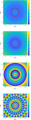 |
Fig. 5 NW2 configuration at λ = 500 nm. Two top panels: intensity diffraction pattern (log10 scale) for the apodized and petal occulters. Two bottom panels: phase diffraction pattern for the apodized and petal occulters. Inside the red circle of diameter 8 m, the petal occulter wavefront is almost identical to the apodized wavefront. |
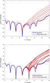 |
Fig. 6 Intensity cuts and comparisons between numerical (top) and theoretical (bottom) calculations for several angular directions between θ = 0 and θ = π/24. |
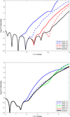 |
Fig. 7 Effect of the number of petals of the Fresnel pattern, cut for the most unfavorable angular direction, for the NW2 (top) and NI2 (bottom) configurations. |
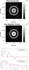 |
Fig. 8 Stray light. Top two panels: residual stray light for a point source star and an example far-resolved 1.5 mas star. For the resolved star, 481 point sources are used, for the same total intensity as in the point source. Two bottom panels: radial cuts given in linear scale and log10 scale. Curves are for the NW2 configuration and a centrally obstructed telescope. The wavefront used is that of the apodized occulter. |
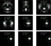 |
Fig. 9 Examples of PSF responses for various point sources (green cross) and the observed PSF maximum (red point). Below 40 mas, these positions do not coincide. After that, there is a shift between these positions until 80 mas. The maximum intensity value and the exact position of the source point that is moved in a single direction are noted in the images. The wavefront used is that of the petal occulter for NW2. |
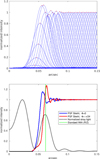 |
Fig. 10 PSFs. Top panel: cuts of PSFs, with the position of the maximum marked by a red dot. Bottom panel: envelope of the maxima μ(ξ), i.e., Strehl, for two directions corresponding to a peak and hollow of petals. The conventional IWA (R/Z) of 0.062 arcsec is indicated by a vertical green line. The stray light corresponding to a resolved 1.5 mas is drawn with the maximum set to 1. |
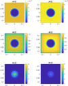 |
Fig. 11 From top to bottom: 2D representations of μ(ξ), ϕ(ξ) and Δ(ξ) obtained for 128 × 128 PSFs in a field of 0.25 × 0.25 arcsec for the petal occulter (left panels) and the apodized occulter (right panels). Data are for NW2 at 500 nm, with a 4m telescope with central obstruction. |
5 Conclusion
The work that we present here has led to several new results and a numerical verification of known theoretical results. We did not calculate our own apodization functions, instead using those of the SISTER (Hildebrandt et al. 2021) NI2 and NW2 configurations. Other configurations could have been studied, such as Cash (2006) or Flamary & Aime (2014).
We show that for an angular field of finite dimension, Fresnel diffraction can be associated with a very low-frequency filter. For a rectangular region, this filter is expressed using cosine and sine Fresnel integrals. For a region of dimension 2L × 2L, this filtering limits the usual Fresnel filter, exp(−iπλzu2), to frequencies lower than uL <~ L/(λZ). More details are shown in Appendix A. In terms of frequency-resolving elements, this can be expressed as twice the Fresnel number corresponding to the whole field of view. For an exoplanet experiment, this condition is easy to satisfy, and we used many more sampling points (8192 in the present study) to obtain a fairly well-sampled representation of the wavefront. We note that for a solar experiment, the necessary number of points would be difficult to obtain, and in that case it would probably be better to use the Maggi–Rubinowicz approach as done by Rougeot (2020).
Despite this low-frequency limitation, the Fourier transform of the occulter must be calculated with great precision. In tests that we have carried out and which are not reported in this paper, if this function is not precisely computed, we observe a deterioration in the dark level of the shadow of the occulter, by of a few orders of magnitude. To understand this necessity, we must consider that in a 2D computation that uses discrete samples, the ratio of 1s and 0s on a circle must be such that the apodization function is recovered. As this function is defined over six digits, this would impose a gigantic number of points for 2D sampling. By reducing the precision of the apodization profile to 4 digits, the shadow level would be increased by a factor of 100. This is the reason why we opted for the continuous Fourier transform technique, where the occulter is approximated with a polygon. This approach was used for radio antennas and detailed in Appendix B.
We compared the diffractions for petal occulters with those for the reference apodized occulter. A key point comes from the fundamental result of Vanderbei et al. (2007), which showed that in the darkest central zone of the petal occulter, the Fresnel diffraction of the petal occulter merges with that of the apodized occulter (i.e., an occulter with variable transmission). Our numerical results were found to agree very well with their theoretical predictions. The centers of the Fresnel diffraction patterns are similar over a fairly large width, a width that increases with the number of petals used. Adding more petals does not improve the center of the shadow, it makes the dark central spot larger.
Once the Fourier transform of the occulter was calculated, it was easy to change the wavelength of the observation by simply changing the Fresnel filtering. From the wavefront thus obtained, we could easily calculate the stray light that spreads over the field, and the PSFs as well. We calculated the stray light for a resolved star and gave an example using 481 point sources inside a 1.5 mas star. However, we can also easily calculate the star leakage for any non-point star. We find that the starshade experiment is not sensitive to star leakage, except that, with a given configuration, there is a limit to the diameter of a star that can be observed: the larger the dark central region, the larger this diameter. An increase in the stellar diameter can be obtained by using more petals; after that, the use of another configuration for very large star diameters becomes necessary. To make this configuration change, the similarity properties of Fresnel diffraction discussed in this paper may be useful.
We give examples of PSFs that can be found elsewhere in the literature. Inside the deep geometric shadow zone, these PSFs are only avatars due to diffraction from the edges of the occulter. The responses are distorted, the intensity levels are very low, and the photocenters of the PSFs do not correspond to the original position of the source points. Beyond the vignetting zone, the PSFs quickly return to an Airy-like shape for a circular telescope. In fact, the illustrations we have given are for a centrally obstructed telescope.
For a fairly large area of the field, including the vignetting zone and beyond, we give maps of the overall characteristics of the PSFs, transmitted flux, maximum values, and equivalent widths (16 384 PSFs computed in these examples). For a perfect system and assuming that the detection limit is photon noise, we also give maps of the S/N. It is clear that there is a central dead zone, where no image recovering will be possible, and a vignetting zone closer to the star than the IWA in its classic definition, where a Fredholm-type image reconstruction could be considered. This is what we propose to do in future work.
One of the unexpected conclusions of this study is that, for a rapid analysis of the effect of a coronagraph with an external occulter, the problem of precision for a starshade calculation can be circumvented to some extent. It is mandatory to calculate the stray light, and for this we can use the apodized profile, using a Hankel transform to get the shape of the wave at the center, for example (ignoring the central dead zone where no image reconstruction is possible). It is, however, necessary to obtain the PSFs in the vignetting zone, beginning in a zone where the flux exceeds a given value, for example 1% of the nominal flux. We can then use a classic filtering technique with just a few thousand or tens of thousands of points, which would be sufficient for the vignetting zone and beyond. The precise calculation of the number of points according to the method given in this paper or developed in SISTER remains mandatory for more precise analyses, for example analysis of occulter micro-defects.
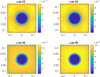 |
Fig. 12 2D representations of the S/N υ(ξ) for 128 × 128 PSFs in a field of 025 × 0.25 arcsec for the petal occulter (left panels) and the apodized occulter (right panels) for the planet-to-star ratio ϵ = 10−12 (top panels) and ϵ = 10−10 (bottom panels). These values are to be multiplied by the square root of the number of photons for the star, |
![Mathematical equation: $\[\sqrt{N_*}\]$](/articles/aa/full_html/2024/06/aa49589-24/aa49589-24-eq22.png)
Acknowledgements
Some of the results in this paper have been derived using starshade simulations from the SISTER (Starshade Imaging Simulation Toolkit for Exoplanet Reconnaissance) package. S.P. thanks Mamadou N'Diaye for enlightening discussions. Thanks are due to the referee for constructive comments.
Appendix A The Fresnel filter for a finite spatial field
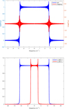 |
Fig. A.1 Illustration of the analytical expression of Eq. A.4 for the parameters of NI2 at λ = 500 nm and Z = 37242 km. Top panel: Real (left y-axis) and imaginary (right y-axis) parts of FL(u) for L = 52, resulting in wL = 2.7925 m−1. Bottom panel: Modulus of FL(u) for the two values L = 52 m and L = 208 m, with uL = 2.7925 m−1 and uL = 10.1179 m−1, respectively. |
We computed the Fourier transform of Eq. 5 for a finite spatial field. It is an integral of separable variable transformations of x to u and of y to υ. We assumed that the functions in x and y are both spatially limited between −L and +L, where L is the area of interest for the diffraction pattern.
For the transform of x into u, we have
![Mathematical equation: $\[\begin{aligned}& \mathcal{F}\left[\frac{1}{\sqrt{i \lambda Z}} \exp \left(i \pi \frac{x^2}{\lambda Z}\right) \Pi\left(\frac{x}{2 L}\right)\right]= \\& \frac{1}{\sqrt{i \lambda Z}} \int_{-L}^{+L} \exp \left(i \pi \frac{x^2}{\lambda Z}\right) \exp (-2 i \pi u x) d x= \\& \frac{1}{\sqrt{i \lambda Z}} \exp \left(-i \pi \lambda Z u^2\right) \int_{-L-\lambda Z u}^{+L-\lambda Z u} \exp \left(i \pi \frac{t^2}{\lambda Z}\right) d t,\end{aligned}\]$](/articles/aa/full_html/2024/06/aa49589-24/aa49589-24-eq23.png) (A.1)
(A.1)
where we have made the change of variable t = x − λZu. By expanding the complex exponential in the real and imaginary parts, the last integral can be expressed using the cosine and sine Fresnel integrals, C and S, defined as
![Mathematical equation: $\[\int_0^h \exp \left(i \frac{\pi t^2}{2}\right) d t=C(h)+i S(h),\]$](/articles/aa/full_html/2024/06/aa49589-24/aa49589-24-eq24.png) (A.2)
(A.2)
and Eq. A.1 can be written as
![Mathematical equation: $\[\mathcal{F}\left[\frac{1}{\sqrt{i \lambda Z}} \exp \left(i \pi \frac{x^2}{\lambda Z}\right) \Pi\left(\frac{x}{2 L}\right)\right]=\exp \left(-i \pi \lambda Z u^2\right) F_L(u)\]$](/articles/aa/full_html/2024/06/aa49589-24/aa49589-24-eq25.png) (A.3)
(A.3)
with
![Mathematical equation: $\[\begin{aligned}F_L(u)= & \frac{1}{\sqrt{2 i}}\left(C\left(\sqrt{\frac{2}{\lambda Z}}(L-\lambda Z u)\right)+C\left(\sqrt{\frac{2}{\lambda z}}(L+\lambda Z u)\right)\right. \\& +i\left(S\left(\sqrt{\frac{2}{\lambda z}}(L-\lambda Z u)\right)+S\left(\sqrt{\frac{2}{\lambda z}}(L+\lambda Z u)\right)\right).\end{aligned}\]$](/articles/aa/full_html/2024/06/aa49589-24/aa49589-24-eq26.png) (A.4)
(A.4)
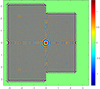 |
Fig. A.2 Numerical illustration of the real parts of the 2D fast Fourier transform of the quadratic phase term of Eq. 4 for NI2 parameters computed for L = 52 m and two λ values, λ = 425 nm (left; uL = 3.2853 m−1) and λ = 552 nm (right; uL = 2.5295 m−1). |
The transform of y into υ can be written using the same function, FL(υ). The Fresnel functions C and S resemble oscillatory sign functions that tend to ±1/2 far from their origins. Due to their composition in Eq. A.4, FL(u) tends to vanish when u is greater than uL,
![Mathematical equation: $\[u_{\mathrm{L}}=\frac{L}{\lambda Z},\]$](/articles/aa/full_html/2024/06/aa49589-24/aa49589-24-eq27.png) (A.5)
(A.5)
and the function FL(ρ) = FL(u)FL(υ) acts as a low pass filter that confines the Fresnel filter of Eq. 5, exp(−iπλz∥ρ∥2), to mainly low frequencies. The value uL, can be converted to the number of significant frequency points, nL, by dividing it by the spectral resolution 1/2L:
![Mathematical equation: $\[n_{\mathrm{L}}=\frac{L / \lambda Z}{1 / 2 L}=2 \frac{L^2}{\lambda Z}=2 \Phi^{\prime},\]$](/articles/aa/full_html/2024/06/aa49589-24/aa49589-24-eq28.png) (A.6)
(A.6)
where Φ′ is the Fresnel number associated with the entire field in which the diffraction is computed. For exoplanet experiments, nL, will be on the order of a few hundred to a few thousand, while it becomes extremely high for the solar case.
An illustration of the FL(u) from Eq. A.4 for the parameters of the NI2 configuration corresponding to an occulter of 26 m in diameter at Z = 37342 km utilized at λ = 500 nm is given in Fig. A.1. In the top panel, we show the real and imaginary parts of FL(u) for the calculation of its diffraction figure for L = 52 m. The bottom panel gives the modulus of FL(u) for the two values L = 52 m and L = 208 m, clearly showing the dependence of uL on L according to Eq. 7.
Figure A.2 shows the real part of the numerical 2D Fourier transform of the Fresnel quadratic phase term limited to 2L × 2L, with L = 52 m for the two extreme λ of the bandwidth considered for NI2 (425nm and 525nm). It shows the dependence of uL on λ, also in agreement with Eq. 7.
This low-frequency behavior of FL(ρ) makes it possible to implement the numerical calculation of the Fourier domain of Eq. 4 and limit the calculation to low frequencies only. In practice, for reasons of good wavefront sampling, we used an array of 8192 × 8192 points, which corresponds to 5 to 10 times nL depending on the configuration and wavelength, λ.
Appendix B Polygonal form factor
Here we present the derivation of Eq. 9, following Wuttke (2021). This result is based on the application of the Stokes formula,
![Mathematical equation: $\[\iint_{\Gamma} \mathrm{d}^2 r \hat{\mathbf{n}}.(\nabla \times \mathbf{g})=\oint_{\partial \Gamma} \mathrm{d} \mathbf{r} \cdot \mathbf{g},\]$](/articles/aa/full_html/2024/06/aa49589-24/aa49589-24-eq29.png) (B.1)
(B.1)
applied to the function ![Mathematical equation: $\[\mathbf{g}=2 \pi \hat{\mathbf{n}} \times \boldsymbol{\rho}\left(e^{i 2 \pi \boldsymbol{\rho.r}}-c\right)\]$](/articles/aa/full_html/2024/06/aa49589-24/aa49589-24-eq30.png) . The left-hand side of the Stokes formula reads
. The left-hand side of the Stokes formula reads
![Mathematical equation: $\[\begin{aligned}\iint_{\Gamma} \mathrm{d}^2 r ~\hat{\mathbf{n}}.(\nabla \times \mathbf{g}) & =4 \pi^2 \hat{\mathbf{n}}.\left[i \boldsymbol{\rho} \times(\hat{\mathbf{n}} \times \boldsymbol{\rho}] \iint_{\Gamma} \mathrm{d}^2 r e^{i 2 \pi \boldsymbol{\rho.r}}\right. \\& =4 \pi^2 i|\hat{\mathbf{n}} \times \boldsymbol{\rho}|^2 \hat{t}(\boldsymbol{\rho}) \\& =4 \pi^2 i \rho^2 \hat{t}(\boldsymbol{\rho}),\end{aligned}\]$](/articles/aa/full_html/2024/06/aa49589-24/aa49589-24-eq31.png)
where ![Mathematical equation: $\[\hat{t}(\boldsymbol{\rho})\]$](/articles/aa/full_html/2024/06/aa49589-24/aa49589-24-eq32.png) , called the polygonal form factor, is the (continuous) Fourier transform of the indicator function of the surface enclosed by the polygon Γ, and ρ = ∥ρ∥. Expressing the right-hand side of the Stokes formula as a sum of integrals over the polygon edges,
, called the polygonal form factor, is the (continuous) Fourier transform of the indicator function of the surface enclosed by the polygon Γ, and ρ = ∥ρ∥. Expressing the right-hand side of the Stokes formula as a sum of integrals over the polygon edges,
![Mathematical equation: $\[\oint_{\partial \Gamma} \mathrm{d}\mathbf{r.g}=\sum_{j-1}^N ~\int_{\mathbf{v}_{j-1}}^{\mathbf{v}_j} \mathrm{d} \mathbf{r.g},\]$](/articles/aa/full_html/2024/06/aa49589-24/aa49589-24-eq33.png) (B.2)
(B.2)
and using an affine parametrization of the edges, rj(λ) = rj + λej, we get
![Mathematical equation: $\[\begin{aligned}\oint_{\partial \Gamma} \mathrm{d} \mathbf{r}. \mathbf{g} & =\sum_{j=1}^N \mathbf{e}_j \cdot \int_{-1}^1 \mathrm{~d} \lambda \mathbf{g}\left(\mathbf{r}_j(\lambda)\right) \\& =2 \pi \sum_{j=1}^N\left[\mathbf{e}_j, \hat{\mathbf{n}}, \boldsymbol{\rho}\right] \int_{-1}^1 \mathrm{~d} \lambda\left(e^{i 2 \pi \boldsymbol{\rho.r}_j(\lambda)}-c\right) \\& =4 \pi \sum_{j=1}^N\left[\hat{\mathbf{n}}, \boldsymbol{\rho}, \mathbf{e}_j\right]\left[\operatorname{sinc}\left(2 \pi \boldsymbol{\rho.e}_j\right) e^{i 2 \pi \boldsymbol{\rho.r}_j}-c\right].\end{aligned}\]$](/articles/aa/full_html/2024/06/aa49589-24/aa49589-24-eq34.png)
Comparing the results for the left- and right-hand sides of Eq. B.1, we get Eq. 9. Now we can justify the role of the additive constant, c, introduced above in function G. We see that ![Mathematical equation: $\[\hat{t}(\boldsymbol{\rho})=2 \sum{_{j=1}^N}\left[~\hat{\mathbf{n}}, \hat{\boldsymbol{\rho}}, \boldsymbol{e}_j\right] \tau\left(\boldsymbol{\rho}, \mathbf{r}_j\right)\]$](/articles/aa/full_html/2024/06/aa49589-24/aa49589-24-eq35.png) , with
, with ![Mathematical equation: $\[\tau\left(\boldsymbol{\rho}, \mathbf{r}_j\right)=\left[\operatorname{sinc}\left(2 \pi \boldsymbol{\rho.e}_j\right) e^{i 2 \pi \boldsymbol{\rho.r}_j}= c] /(2 \pi i \rho)\right.\]$](/articles/aa/full_html/2024/06/aa49589-24/aa49589-24-eq36.png) , and
, and ![Mathematical equation: $\[\hat{\boldsymbol{\rho}}=\boldsymbol{\rho} / \rho\]$](/articles/aa/full_html/2024/06/aa49589-24/aa49589-24-eq37.png) . In the limit ρ → 0, we have
. In the limit ρ → 0, we have
![Mathematical equation: $\[\tau\left(\boldsymbol{\rho}, \mathbf{r}_j\right)=\frac{(1-c)}{2 \pi i \rho}+\hat{\boldsymbol{\rho}}. \mathbf{r}_j+\boldsymbol{\mathcal{O}}(\rho).\]$](/articles/aa/full_html/2024/06/aa49589-24/aa49589-24-eq38.png) (B.3)
(B.3)
Therefore, using c = 1 in the small ρ limit avoids any numerical divergences. We note that in Eq. 10, for a polygon with central symmetry, there are no divergent terms in that limit, and therefore there is no need to introduce additive constants to g.
References
- Aime, C. 2005, A&A, 434, 785 [NASA ADS] [CrossRef] [EDP Sciences] [Google Scholar]
- Aime, C. 2013, A&A, 558, A138 [NASA ADS] [CrossRef] [EDP Sciences] [Google Scholar]
- Aime, C., Theys, C., Rougeot, R., & Lantéri, H. 2019, A&A, 622, A212 [NASA ADS] [CrossRef] [EDP Sciences] [Google Scholar]
- Arenberg, J. W., Harness, A. D., & Jensen-Clem, R. M. 2021, J. Astron. Telescopes Instrum. Syst., 7, 021201 [NASA ADS] [Google Scholar]
- Barnett, A. H. 2021, J. Astron. Telescopes Instrum. Syst., 7, 021211 [NASA ADS] [Google Scholar]
- Born, M., & Wolf, E. 2013, Principles of Optics: Electromagnetic Theory of Propagation, Interference and Diffraction of Light (Elsevier) [Google Scholar]
- Brueckner, G. E., Howard, R. A., Koomen, M. J., et al. 1995, Sol. Phys., 162, 357 [NASA ADS] [CrossRef] [Google Scholar]
- Cady, E. 2012, Opt. Expr., 20, 15196 [NASA ADS] [CrossRef] [Google Scholar]
- Cash, W. 2006, Nature, 442, 51 [NASA ADS] [CrossRef] [Google Scholar]
- Evans, J. W. 1948, J. Opt. Soc. Am., 38, 1083 [NASA ADS] [CrossRef] [Google Scholar]
- Flamary, R., & Aime, C. 2014, A&A, 569, A28 [NASA ADS] [CrossRef] [EDP Sciences] [Google Scholar]
- Goodman, J. W. 1968, Introduction to Fourier Optics. Goodman (McGraw-Hill) [Google Scholar]
- Harness, A., Shaklan, S., Cash, W., & Dumont, P. 2018, JOSA A, 35, 275 [NASA ADS] [CrossRef] [Google Scholar]
- Hildebrandt, S. R., Shaklan, S. B., Cady, E. J., & Turnbull, M. C. 2021, J. Astron. Telescopes Instrum. Syst., 7, 021217 [NASA ADS] [Google Scholar]
- Koomen, M. J., Detwiler, C. R., Brueckner, G. E., Cooper, H. W., & Tousey, R. 1975, Appl. Opt., 14, 743 [NASA ADS] [CrossRef] [Google Scholar]
- Koutchmy, S. 1988, Space Sci. Rev., 47, 95 [NASA ADS] [CrossRef] [Google Scholar]
- Lamy, P., Damé, L., Vivès, S., & Zhukov, A. 2010, SPIE Conf. Ser., 7731, 773118 [NASA ADS] [Google Scholar]
- Lee, S.-W., & Mittra, R. 1983, IEEE Trans. Antennas Propag., 31, 99 [CrossRef] [Google Scholar]
- Lyot, B. 1933, J. R. Astron. Soc. Can., 27, 265 [Google Scholar]
- Mas, D., Perez, J., Hernández, C., et al. 2003, Opt. commun., 227, 245 [NASA ADS] [CrossRef] [Google Scholar]
- Newkirk, G., Jr., & Bohlin, J. D. 1965, in IAU Symp., 23, Astronomical Observations from Space Vehicles, ed. J.-L., Steinberg, 287 [Google Scholar]
- Renotte, E., Baston, E. C., Bemporad, A., et al. 2014, in Space Telescopes and Instrumentation 2014: Optical, Infrared, and Millimeter Wave, 9143, Proc. SPIE, 91432M [Google Scholar]
- Rougeot, R. 2020, PhD thesis, Université Côte d'Azur, France [Google Scholar]
- Rougeot, R., & Aime, C. 2018, A&A, 612, A80 [NASA ADS] [CrossRef] [EDP Sciences] [Google Scholar]
- Rougeot, R., Flamary, R., Galano, D., & Aime, C. 2017, A&A, 599, A2 [NASA ADS] [CrossRef] [EDP Sciences] [Google Scholar]
- Theys, C., Aime, C., Rougeot, R., & Lantéri, H. 2022, A&A, 665, A109 [NASA ADS] [CrossRef] [EDP Sciences] [Google Scholar]
- Tousey, R. 1965, Ann. Astrophys., 28, 600 [NASA ADS] [Google Scholar]
- Vanderbei, R. J., Cady, E., & Kasdin, N. J. 2007, ApJ, 665, 794 [NASA ADS] [CrossRef] [Google Scholar]
- Wuttke, J. 2021, J. Appl. Crystallogr., 54, 580 [NASA ADS] [CrossRef] [Google Scholar]
All Figures
|
Fig. 1 Illustration of the convolution in Eq. (2) where the transparent occulter t(r) from Eq. (1) of size 2R × 2R sweeps the quadratic phase (real part here) shown for a region 2L × 2L. The occulter corresponds to the NI2 configuration. Because of edge effects, the convolution is obtained in the region limited to 2(L − R) × 2(L − R). |
| In the text | |
|
Fig. 2 Comparison between cuts of the intensity diffraction pattern for the apodized occulter of the NW2 configuration at 500 nm (central shadow, log10 scale). The red curve, computed using a Hankel transform, is almost identical to the blue curve, which is a radial cut of the pattern obtained using 2D Fourier transforms. |
| In the text | |
|
Fig. 3 Intensity diffraction pattern (linear scale) for the NI2 configuration at λ = 500 nm. Top panels: 2D representations of a zone of 80 × 80 m for the apodized occulter (top panel) and the petal occulter (second panel). Bottom two panels: radial cuts for the angles θ = 0 and θ = π/24. The strong variations for the petal occulter contrast with the smooth variations for the apodized occulter. |
| In the text | |
|
Fig. 4 Variation with λ from 425 to 552 nm of a periodic angular sector anamorphosed to a rectangle in the coordinates ∥r∥ × θ, ∥r∥ from 0 to 23 m, θ from 0 to π/12, and corresponding to the periodicity of the 24-petal occulter. |
| In the text | |
|
Fig. 5 NW2 configuration at λ = 500 nm. Two top panels: intensity diffraction pattern (log10 scale) for the apodized and petal occulters. Two bottom panels: phase diffraction pattern for the apodized and petal occulters. Inside the red circle of diameter 8 m, the petal occulter wavefront is almost identical to the apodized wavefront. |
| In the text | |
|
Fig. 6 Intensity cuts and comparisons between numerical (top) and theoretical (bottom) calculations for several angular directions between θ = 0 and θ = π/24. |
| In the text | |
|
Fig. 7 Effect of the number of petals of the Fresnel pattern, cut for the most unfavorable angular direction, for the NW2 (top) and NI2 (bottom) configurations. |
| In the text | |
|
Fig. 8 Stray light. Top two panels: residual stray light for a point source star and an example far-resolved 1.5 mas star. For the resolved star, 481 point sources are used, for the same total intensity as in the point source. Two bottom panels: radial cuts given in linear scale and log10 scale. Curves are for the NW2 configuration and a centrally obstructed telescope. The wavefront used is that of the apodized occulter. |
| In the text | |
|
Fig. 9 Examples of PSF responses for various point sources (green cross) and the observed PSF maximum (red point). Below 40 mas, these positions do not coincide. After that, there is a shift between these positions until 80 mas. The maximum intensity value and the exact position of the source point that is moved in a single direction are noted in the images. The wavefront used is that of the petal occulter for NW2. |
| In the text | |
|
Fig. 10 PSFs. Top panel: cuts of PSFs, with the position of the maximum marked by a red dot. Bottom panel: envelope of the maxima μ(ξ), i.e., Strehl, for two directions corresponding to a peak and hollow of petals. The conventional IWA (R/Z) of 0.062 arcsec is indicated by a vertical green line. The stray light corresponding to a resolved 1.5 mas is drawn with the maximum set to 1. |
| In the text | |
|
Fig. 11 From top to bottom: 2D representations of μ(ξ), ϕ(ξ) and Δ(ξ) obtained for 128 × 128 PSFs in a field of 0.25 × 0.25 arcsec for the petal occulter (left panels) and the apodized occulter (right panels). Data are for NW2 at 500 nm, with a 4m telescope with central obstruction. |
| In the text | |
|
Fig. 12 2D representations of the S/N υ(ξ) for 128 × 128 PSFs in a field of 025 × 0.25 arcsec for the petal occulter (left panels) and the apodized occulter (right panels) for the planet-to-star ratio ϵ = 10−12 (top panels) and ϵ = 10−10 (bottom panels). These values are to be multiplied by the square root of the number of photons for the star, |
| In the text | |
|
Fig. A.1 Illustration of the analytical expression of Eq. A.4 for the parameters of NI2 at λ = 500 nm and Z = 37242 km. Top panel: Real (left y-axis) and imaginary (right y-axis) parts of FL(u) for L = 52, resulting in wL = 2.7925 m−1. Bottom panel: Modulus of FL(u) for the two values L = 52 m and L = 208 m, with uL = 2.7925 m−1 and uL = 10.1179 m−1, respectively. |
| In the text | |
|
Fig. A.2 Numerical illustration of the real parts of the 2D fast Fourier transform of the quadratic phase term of Eq. 4 for NI2 parameters computed for L = 52 m and two λ values, λ = 425 nm (left; uL = 3.2853 m−1) and λ = 552 nm (right; uL = 2.5295 m−1). |
| In the text | |
Current usage metrics show cumulative count of Article Views (full-text article views including HTML views, PDF and ePub downloads, according to the available data) and Abstracts Views on Vision4Press platform.
Data correspond to usage on the plateform after 2015. The current usage metrics is available 48-96 hours after online publication and is updated daily on week days.
Initial download of the metrics may take a while.