| Issue |
A&A
Volume 686, June 2024
|
|
|---|---|---|
| Article Number | A165 | |
| Number of page(s) | 7 | |
| Section | Astrophysical processes | |
| DOI | https://doi.org/10.1051/0004-6361/202348766 | |
| Published online | 07 June 2024 | |
Secondary cosmic-ray nuclei in the Galactic halo model with nonlinear Landau damping
1
I. E. Tamm Theoretical Physics Division of P. N. Lebedev Institute of Physics, 119991 Moscow, Russia
e-mail: This email address is being protected from spambots. You need JavaScript enabled to view it.
2
Max-Planck-Institut für Extraterrestrische Physik, 85748 Garching, Germany
e-mail: This email address is being protected from spambots. You need JavaScript enabled to view it.
Received:
28
November
2023
Accepted:
16
March
2024
Abstract
We employed our recent model of the cosmic-ray (CR) halo to compute the Galactic spectra of stable and unstable secondary nuclei. In this model, confinement of the Galactic CRs is entirely determined by the self-generated Alfvénic turbulence whose spectrum is controlled by nonlinear Landau damping. We analyzed the physical parameters affecting propagation characteristics of CRs and estimated the best set of free parameters providing accurate description of available observational data. We also show that agreement with observations at lower energies may be further improved by taking into account the effect of ion-neutral damping that operates near the Galactic disk.
Key words: cosmic rays / Galaxy: halo
© The Authors 2024
 Open Access article, published by EDP Sciences, under the terms of the Creative Commons Attribution License (https://creativecommons.org/licenses/by/4.0), which permits unrestricted use, distribution, and reproduction in any medium, provided the original work is properly cited.
This article is published in open access under the Subscribe to Open model.
Open access funding provided by Max Planck Society.
1. Introduction
In our recent papers, Dogiel et al. (2020) and Chernyshov et al. (2022), we developed a self-consistent model of the cosmic-ray halo where confinement of the Galactic cosmic rays (CRs) is entirely determined by the self-generated Alfvénic turbulence. Following Ptuskin et al. (1997), we assumed that the spectrum of Alfvén waves excited via the resonant streaming instability is controlled by nonlinear Landau damping (Chernyshov et al. 2022). We showed that variations seen in the measured spectral index of CR protons at ≲105 GeV can be accurately explained by the height dependence of the plasma beta – the key parameter controlling the magnitude of nonlinear Landau damping (Lee & Völk 1973; Miller 1991).
There have been a number of different physical models proposed to explain the observed variations in the spectral index of protons and heavier nuclei in this energy range. In particular, these include scenarios of the spectral break in the CR injection spectra as well as of local sources at low and high energies (Vladimirov et al. 2012; Fornieri et al. 2021a); different mechanisms for CR confinement at different energies, which are associated with scattering on both self-generated and pre-existing MHD turbulence (Aloisio et al. 2015; Evoli et al. 2018; Fornieri et al. 2021b; Kempski & Quataert 2022); a local supernova remnant as an additional CR source (e.g., Erlykin & Wolfendale 2015; Yang & Aharonian 2019; Liu et al. 2019); and CR reacceleration at a stellar bow shock (Malkov & Moskalenko 2021, 2022). Therefore, the aim of the present paper is to explore the ability of our model to reproduce the measured spectra of heavier CR nuclei.
Apart from available observational data on primary CRs, additional information about CR transport in the Galactic halo can be derived from the data on secondary nuclei, which include isotopes of Li, Be, and B. The abundance of these nuclei in CRs is much greater than in the interstellar medium, and they are believed to be produced by nuclear interactions of primary CRs with background gas (see, e.g., the review by Strong et al. 2007). The boron-to-carbon ratio is normally employed to test CR propagation models, since boron is mostly produced from carbon and cross-sections for boron production are well known.
Propagation of CRs can be further constrained by studying unstable CR isotopes. Hayakawa et al. (1958) suggested that the abundance of unstable 10Be contains information on how long CRs are confined in the Galactic halo. Since the decay time of the unstable isotope is estimated to be comparable to the confinement time, the abundance ratio 10Be/9Be must be a strong function of the confinement time and thus can be used to derive characteristics of the CR halo. The downside of this approach is that observations require careful separation of the two isotopes, which is a complicated task.
In this paper, we applied our self-consistent model by Chernyshov et al. (2022) to compute the Galactic spectra of stable and unstable secondary nuclei. We explored the physical parameters affecting propagation characteristics of CRs and estimated the best set of free parameters, which allowed us to accurately describe available observational data.
2. Governing equations for CR nuclei
GALPROP1 (Moskalenko & Strong 1998) is one of the most sophisticated numerical codes employed to calculate spectra of CR species in the Galaxy. For our purposes, however, GALPROP cannot be directly used due to the following reasons. First, the magnitude and the energy dependence of the diffusion coefficient D in GALPROP are assumed, and D is set to be constant in space – whereas in Chernyshov et al. (2022)D(p, z) is a solution of a self-consistent model, resulting in a strong dependence on the vertical coordinate z. Second, GALPROP utilizes cylindrical or 3D geometry, while our model is one-dimensional. Therefore, below we numerically solve a set of transport equations for the primary and secondary CR nuclei, using the self-consistent solution for protons from Chernyshov et al. (2022) and utilizing the nuclear reaction network from GALPROP.
To describe propagation of CR nuclei i, we use the one-dimensional transport equation for their spectrum Ni(p, z):
 (1)
(1)
where R = pc/eZi is the rigidity, related to the momentum p via the atomic number Zi. The term Ṙi(R) ≡ ṗi(R)c/eZi < 0 describes continuous momentum losses due to ionization and Coulomb collisions. The timescales τfr, i(R) and τdec, i are, respectively, the fragmentation time of nuclei i due to their collisions with background gas and the decay time (in case of unstable nuclei). The former is given by 1/τfr, i = nHσfr, ivi, where nH is the gas number density, vi is the velocity of the nuclei, and σfr, i(R) is the fragmentation cross section.
The diffusion coefficient Di of nuclei i is proportional to the product of the velocity vi and the mean free path that is a sole function of rigidity (for a given z). Therefore, Di is related to the diffusion coefficient of protons Dp via
 (2)
(2)
while the ratio of vi to the proton velocity vp is
 (3)
(3)
where Ai is the atomic mass of the nuclei. The dependence Dp(R, z), derived from our self-consistent model (Chernyshov et al. 2022), sets the spatial profile of the proton spectrum in the halo, Np(R, z) (see Sect. 3). The advection velocity uadv is assumed to be equal to the local Alfvén velocity uA in the halo, vanishing discontinuously at the disk boundary z = zd,
 (4)
(4)
where θ(z) is the Heaviside function.
The source terms Qi(R, z) and qi(R) describe the production of, respectively, primary CR nuclei and secondary nuclei. The source term Qi can be approximated by
 (5)
(5)
where the spectral index γ is the same for all primary nuclei, and δ(z) is the delta function. Constants Ci are adjusted to fit observational data on primary CR spectra, and Ci = 0 for secondary nuclei. The source term qi has two contributions. One is associated with the fragmentation of primary CRs due to their collisions with background gas:
 (6)
(6)
where σji is the total inclusive cross-section of production of secondary nuclei i from nuclei j. The product σjiNj is evaluated at  , which takes into account the fact that nuclear reactions conserve the kinetic energy (momentum) per nucleon, not the rigidity. Similarly, the second contribution due to decay of unstable nuclei is given by
 (7)
(7)
We use the advection velocity uadv(z) and the proton diffusion coefficient Dp(R, z) from the self-consistent model by Chernyshov et al. (2022). The diffusion coefficients Di for heavier nuclei are calculated from Eq. (2). To estimate the momentum loss terms Ṙi(R), the fragmentation cross-sections σfr, i(R), and the total inclusive cross sections σji(R), we use the GALPROP code (energy_losses.cc, nucleon_cs.cc, and decayed_cross_sections.cc, respectively).
The set of Eq. (1) with the secondary source terms (6) and (7) is solved numerically until a stationary solution is reached. To reduce computation time, we take into account only the following primary nuclei: 4He, 12C, 14N, 16O, 20Ne, 24Mg, 28Si, 32S, and 56Fe; for secondary nuclei, we consider 6Li, 7Li, 7Be, 9Be, 10Be, 10B, 11B, 13C, 14C, 15N, 17O, and 18O.
We note that the unstable nuclei 7Be decay via the electron capture, with the lifetime of about 100 days for hydrogen-like ions formed after recombination with the surrounding electrons. Therefore, for our purposes we assume that 7Be nuclei decay immediately after recombination. This assumption is well justified, because for these nuclei we are only interested in the kinetic energies below ∼103 GeV/nucleon. The electron recombination cross-section from GALPROP is added to the fragmentation cross-section of 7Be and also used as the production cross-section for the reaction 7Be + e → 7Li.
3. Analytical estimates for primary and secondary CR spectra
In this section, we briefly summarize predictions of Chernyshov et al. (2022) for spectra of primary CR nuclei, and we apply these to derive and analyze simple scaling relations for stable and unstable secondary nuclei. Similarly to approaches applied earlier to constrain diffusion parameters in the halo (see, e.g., Maurin et al. 2001), this allows us to compare the theoretical predictions with observations and put constrains on our self-consistent model (see Sect. 4).
The one-dimensional model by Chernyshov et al. (2022) considers two regions: the Galactic disk, located at 0 ≤ z ≤ zd and the Galactic halo at z > zd. The advection velocity in the halo equals to the Alfvén velocity uA(z), and continuous momentum losses vanish in this region. All sources of primary CRs are located in the disk, where we assume CR diffusion in the vertical direction with the diffusion coefficient Dd. Also, we suppose that turbulence in the disk is characterized by zero cross-helicity (that is, spectra of waves propagating in both directions are balanced), and, hence, advection is absent. For simplicity, we neglect the vertical gradient of CR density in the disk. The latter implies the following necessary condition for the fragmentation and decay timescales:
 (8)
(8)
We point out that this condition is satisfied for values of Dd ∼ 1028 cm2 s−1 (typically assumed for GeV particles), and therefore the results presented in Sect. 4 do not depend on the particular choice of Dd.
In Chernyshov et al. (2022), we calculated the outflow velocity for protons up(R, z) self-consistently; this relates the proton spectrum in the halo Np(R, z) to the outgoing flux of protons at the disk boundary, Sp(R),
 (9)
(9)
where
 (10)
(10)
and η(R, z) is a dimensionless variable:
 (11)
(11)
According to Eqs. (3) and (23) in Chernyshov et al. (2022), we have Dp(R, z)∝ − g(z)/[R2Sp(R)]′, where g(z) describes the height dependence of nonlinear Landau damping (see Eq. (7) therein), and the prime denotes the derivative with respect to R. The function g(z) plays a key role in shaping the self-consistent proton spectrum and determining the energy dependence of the halo size (see Chernyshov et al. 2022, for details): g and hence Dp decrease with z while uA increases. Thus, the upper halo boundary is set where the advection contribution uANp to the outgoing proton flux becomes equal to the diffusion contribution −Dp∂Np/∂z, which is equivalent to the condition η(R, z)∼1.
The outflow velocity ui(R, z) for heavier primary species only deviates from up(R, z) due to the factor vi/vp in the diffusion coefficient, Eq. (2). For the estimates below, we assume relativistic particles with vi ≈ c ≈ vp; it is thus safe to set Di ≈ Dp and ui ≈ up.
Furthermore, continuous momentum losses operating in the disk are negligible for protons with the kinetic energy above ∼0.5 GeV (Chernyshov et al. 2022), and the outgoing flux in this case is equal to the accumulated source of protons in the disk (see Eq. (20) therein;  in our notations). The threshold rigidity Rth, above which the losses are negligible for heavier nuclei, scales as
  for sub-relativistic particles and Rth ∝ Zi in the ultra-relativistic limit. In our analysis (see Sect. 4), we are interested in rigidity values of up to ∼105 GeV, and thus the effect of continuous losses can be reasonably neglected.
We first consider stable secondary nuclei. By integrating Eq. (1) across the disk and matching the resulting flux at the disk boundary with the outgoing flux according to Eq. (9), we can estimate the secondary spectra N0(R) = N(R, zd) in the disk:
 (12)
(12)
(here and below, nuclei index i is omitted for brevity). The numerator, which is the integral over the secondary source term, is proportional to the vertical column density of hydrogen atoms in the disk, 𝒩H = nHzd; the denominator is a sum of the outflow velocity at the disk boundary, u0(R) = up(R, zd), and the velocity scale ufr(R) = 𝒩Hσfr(R)v ≡ zd/τfr(R) is associated with fragmentation of the secondary nuclei. After substituting Eq. (6) for qfr(R), the obtained expression allows us to estimate abundance ratios of secondary-to-primary nuclei and compare them with available measurements. Keeping in mind that qfr(R) and ufr(R) have similar dependencies on rigidity (since both scale with σji(R), similar for different nuclei), whereas observations generally exhibit a strong dependence of the secondary to primary ratios on R, we conclude that u0 must be substantially larger than ufr. Hence, for assumed values of 𝒩H, observations yield the dependence u0(R) that can be compared with the prediction of Chernyshov et al. (2022).
Equation (12) cannot be used for unstable nuclei, since their flux in the halo is not conserved, and thus Eq. (9) is no longer applicable. To take into account the decay, one can introduce the “survival probability” P(R, z), which relates the spectrum of unstable nuclei N*(R, z) in the halo to their outgoing flux S*(R) at the disk boundary:
 (13)
(13)
The outflow velocity u(R, z) is given by Eq. (10), while the unknown value of S*(R) is calculated from the matching condition for the flux at z = zd.
Substituting Eq. (13) in Eq. (1) leads to the following equation for P(R, z) in the halo:
 (14)
(14)
By introducing a new dimensionless variable  , we obtain
 (15)
(15)
Then, by assuming  and
and  , we reduce it in the Shrödinger equation,
 (16)
(16)
which can be solved using the WKB method. The necessary condition for the WKB method to be applied is that the “potential” on the rhs of Eq. (16) varies sufficiently slowly with y, that is,
 (17)
(17)
which leads to
 (18)
(18)
The lhs of this condition can be considered as characteristic halo size; according to Dogiel et al. (2020), the upper halo boundary either forms due to a sudden increase in the diffusion coefficient – which reflects a transition to CR free-streaming in Eq. (1) – or it is set where the advection contribution uAN to the outgoing flux starts dominating. The rhs is roughly the characteristic height that unstable nuclei can reach. Thus, the necessary condition for the WKB approximation to be applicable requires τdec to be small enough that unstable nuclei are not reaching the halo boundary.
Substituting the leading term of the WKB solution for  and keeping in mind that P(R, z) should be finite at z = ∞ (as sources of unstable nuclei are absent in the halo), we obtain
![Mathematical equation: $$ \begin{aligned} P \approx A\left(\frac{u^2\tau _{\rm dec}}{D}\right)^{1/4}\exp \left[\;\int \limits _{z_{\rm d}}^z \left(\frac{u}{D} - \frac{1}{\sqrt{D\tau _{\rm dec}}}\right) \mathrm{d}z_1\right], \end{aligned} $$](/articles/aa/full_html/2024/06/aa48766-23/aa48766-23-eq26.gif) (19)
(19)
where the constant A is calculated from the boundary condition at z = zd,
 (20)
(20)
This yields the following expression for P0(R)≡P(R, zd):
 (21)
(21)
where D0(R)≡D(R, zd), u0(R)≡u(R, zd), and small terms are omitted according to Eq. (18). We note that P0 is always much smaller than unity (and thus is a function of D0 and u0) if the WKB condition (18) is satisfied in the advection-dominated regime.
Spectra of unstable nuclei in the disk,  , are estimated using a matching condition for their flux, similar to that used to derive Eq. (12). Assuming that condition (8) is satisfied, we integrate Eq. (1) across the disk and, employing Eq. (13), obtain
![Mathematical equation: $$ \begin{aligned} N_0^*(R) = \frac{P_0(R)q(R)z_{\rm d}}{u_0(R) + P_0(R)\left[u_{\rm fr}(R) + z_{\rm d}/\tau _{\rm dec}\right]}, \end{aligned} $$](/articles/aa/full_html/2024/06/aa48766-23/aa48766-23-eq30.gif) (22)
(22)
where q = qfr + qdec according to Eqs. (6) and (7). As discussed after Eq. (12), observational data suggest that u0 ≳ ufr, and therefore the term ufr ≡ zd/τfr can also be dropped in Eq. (22). Then two limits can be considered. One is when τdec is too small and the contribution of the second term in the brackets, P0zd/τdec, is much larger than u0. In this “useless” case,  depends neither on u0 nor on P0; therefore, it does not contain information on the diffusion coefficient. In the opposite limit, if
 (23)
(23)
and condition (18) is satisfied, abundance ratios of unstable to stable secondary nuclei derived from Eqs. (12) and (22) are proportional to  . Hence, the results can be compared with a rigidity dependence deduced from observational data, which allows us to verify the model prediction of Chernyshov et al. (2022). Comparison with beryllium and boron measurements are particularly convenient here, as boron is partially produced due to decay of 10Be. We point out that if τdec ≪ τfr, then condition (23) is equivalent to the initial necessary condition (8) of homogeneity within the disk.
The main results of the simple analysis presented in this section can be summarized as follows.
-
Measured abundance ratios of stable secondary-to-primary nuclei can be used to verify the expression for the outflow velocity u0(R), which is derived from the self-consistent model by Chernyshov et al. (2022). Below, we employ the B/C ratio for this purpose.
-
Measured abundance ratios of unstable-to-stable secondary nuclei can be used to verify the derived diffusion coefficient D0(R) and, thus, the predicted size of the halo. Such analysis is possible if the decay timescale τdec of unstable nuclei is within a certain range, satisfying conditions (18) and (23). Here, one can either use the Be/B ratio, since Be includes unstable 10Be, or the 10Be/9Be ratio directly if observational data are available.
4. Discussion
In this section, we present and discuss results of numerical solution of Eq. (1), and compare this with available observational data.
4.1. Numerical results and comparison with observations
We employ the self-consistent halo model by Chernyshov et al. (2022) with a two-component vertical distribution of ionized gas, which provides the best agreement with observations. The two components include a warm-ionized-medium (WIM) phase  with constant temperature TWIM and a hot-gas phase
  with constant temperature Thot.
The vertical distribution of neutral gas in the disk is taken from GALRPOP at the galactocentric radius of 8 kpc, and we multiplied it by a numerical factor χn of about unity, which is needed to fit the B/C ratio. This factor accounts for the effect of diffusion along the Galactic disk. The vertical magnetic field is considered to be constant. In the injection term of primary nuclei, Eq. (5), each normalization constant Ci is adjusted to fit observational data. We assume γ = 2.26 for the spectral index of all heavier nuclei, which is slightly different from that of protons, γp = 2.32. For a given set of model parameters, possible variations in γ and γp are limited by error bars for the observational data: according to Aguilar et al. (2021), Δγ assessed for helium is ≪0.05 while Δγp ∼ 0.01.
We note that the density factor χn is a global parameter of the model. It affects all nuclei (including low-energy protons via continuous losses), and therefore iterative runs are needed to compute the spectra. The first run is made with χn = 1. This allows us to assess the required correction by comparing the measured B/C ratio with the computed ratio, and use the updated value of χn for the next run. Since the resulting value of χn is close to unity, we do not perform further iterations.
To provide the best fit to the new data on proton spectrum reported by CALET (Adriani et al. 2022a), we slightly adjusted parameters of our original paper (Chernyshov et al. 2022). For the vertical magnetic field in the halo we keep using the value of B = 1 μG, according to the order-of-magnitude estimates by Jansson & Farrar (2012). The updated parameters of two-component ionized gas, based on observations reported in Ferrière (1998) and Gaensler et al. (2008), are  cm−3, zWIM = 0.4 kpc, TWIM = 0.7 eV,
  cm−3, zhot = 2 kpc, and Thot = 200 eV. The resulting proton spectrum is plotted in the upper panel of Fig. 1 by the dashed line together with the observational data, taken from AMS-02 (Aguilar et al. 2015), CALET (Adriani et al. 2019), NUCLEON-KLEM (Grebenyuk et al. 2019), CREAM-I (Yoon et al. 2011), CREAM-I+III (Yoon et al. 2017), and DAMPE (An et al. 2019). The data are collected using Cosmic-Ray DataBase (CRDB v4.0) by Maurin et al. (2020). The lower panel shows the computed halo size, set at the height where η(R, z) = 1 (Chernyshov et al. 2022).
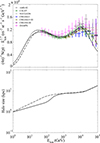 |
Fig. 1. Energy spectrum of CR protons (upper panel) and energy-dependent halo size (lower panel), derived from the self-consistent model by Chernyshov et al. (2022) without (dashed line) and with (solid line) taking into account the ion-neutral damping. The symbols in the upper panel depict the observational data. |
The results of the numerical solution of Eq. (1) for the above set of parameters are represented in Fig. 2 by the dashed lines. The observational data are taken from AMS-02 (Aguilar et al. 2016, 2021), BESS-PolarII (Abe et al. 2016), CALET (Adriani et al. 2023, 2022b), CREAM-II (Ahn et al. 2009), CREAM-I+III (Yoon et al. 2017), DAMPE (Alemanno et al. 2021; DAMPE Collaboration 2022; Parenti et al. 2023), NUCLEON-KLEM (Grebenyuk et al. 2019), and PAMELA (Adriani et al. 2011, 2014) using Cosmic-Ray DataBase (CRDB v4.1) by Maurin et al. (2020, 2023). For 10Be/9Be, we use preliminary AMS-02 data reported by Derome & Paniccia (2021) and their recent update by Wei (2023), as well as ISOMAX data (Hams et al. 2004), all available only for relatively low rigidities. To account for the solar modulation, we use the force-field approximation with potential ϕ = 0.5 GeV (Gleeson & Axford 1968). Our self-consistent model shows reasonable agreement with the observational data for R ≳ 30 GeV. To fit the B/C ratio, the density distribution from GALPROP is multiplied by the factor of χn = 0.85.
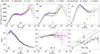 |
Fig. 2. Spectra of nuclei and their ratios versus rigidity. Top panels: spectra of primary CR nuclei of helium (a), carbon (b), and nitrogen (c). Bottom panels: abundance ratios of stable secondary to primary nuclei, represented by the boron-to-carbon ratio (d), as well as of unstable to stable secondary nuclei, represented by the beryllium-to-boron (e) and the beryllium-10-to-beryllium-9 (f) ratios. Our numerical results without and with taking into account the ion-neutral damping are plotted, respectively, by the dashed and solid lines. The symbols depict the observational data: preliminary AMS-02 data for the 10Be/9Be ratio (Derome & Paniccia 2021) and their recent update (Wei 2023) are represented in the bottom right panel by the black crosses and squares, respectively. |
We see that the agreement is also good for abundance ratios including unstable secondary nuclei, such as Be/B. However, for a pure unstable-to-stable ratio of 10Be/9Be our results substantially overestimate the values deduced from preliminary AMS-02 data by Derome & Paniccia (2021) and Wei (2023). Given that the B/C ratio (solely determined by u0(R) in our model) is well reproduced, the discrepancy in the 10Be/9Be ratio may indicate that our model significantly underestimates D0(R) in the measured range of rigidities.
4.2. Effect of ion-neutral damping
In Sect. 4.1, we assumed that turbulence is solely regulated by nonlinear Landau damping. There are, of course, other damping mechanisms that may contribute, such as viscous and turbulent damping as well as ion-neutral damping (see, e.g., Kulsrud & Pearce 1969; Xu & Lazarian 2022). However, in Dogiel et al. (2020) we showed that viscous and turbulent damping can be safely neglected in the CR halo.
On the other hand, the ion-neutral damping may substantially affect the excitation-damping balance for MHD waves near the Galactic disk, suppressing the turbulence and, thus, increasing the value of diffusion coefficient D0(R). This effect can be included in the excitation-damping balance Eq. (21) of Chernyshov et al. (2022) by adding the ion-neutral friction rate νin to the rhs of that equation. The energy density of MHD fluctuations is then described by their modified Eq. (22), indicating that turbulence at longer wavelengths can be completely damped. Since νin is proportional to the neutral gas density, the damping rapidly decreases with the height, and hence turbulence at larger z remains practically unaffected.
To explore the effect of ion-neutral damping on the diffusion coefficient as well as on the outflow velocity and spectra of protons and nuclei, we first solve a set of self-consistent equations by Chernyshov et al. (2022) with the additional term νin in the excitation-damping balance. Then, we adjust the model parameters to be consistent with measurements. The best fit to the data in this case is achieved for a slightly lower temperature of the hot phase, Thot = 170 eV (instead of 200 eV) and a slightly larger scale height: zhot = 2.3 kpc (instead of 2 kpc). Also, the spectral index of proton sources is increased to γp = 2.42 (from 2.32) to compensate for a more efficient escape of low-energy particles. The resulting proton spectrum and the halo size are plotted in Fig. 1 by the solid lines.
Next, we numerically solve Eq. (1) using the computed diffusion coefficient and adjust the model parameters for nuclei sources. The spectral index of primary nuclei is now set to γ = 2.37 (instead of 2.26). The value of χn is adjusted as well, as the ion-neutral damping stimulates escape from the disk, which needs to be compensated by enhanced production of secondary nuclei. Therefore, the density factor to fit the B/C ratio is now χn = 1.15 (instead of 0.85). The results are shown in Fig. 2 by the solid lines. One can see that the inclusion of ion-neutral damping makes the agreement with the observations noticeably better, in particular for the 10Be/9Be ratio.
It is worth noting that the difference between the solid and dashed lines at R ≳ 104 GeV, seen in Figs. 1 and 2 for the primary CR spectra, can be eliminated if we also take into account a decrease of the magnetic field with the height (neglected above for simplicity). The lower panel of Fig. 1 shows that the halo size exceeds ∼10 kpc for R ≳ 104 GeV, and the expected field decrease at such heights should lead to the proportional reduction of uA(z) (relative to the dependence assumed above); according to Eq. (9), this should proportionally increase the CR spectrum at the upper halo boundary and, thus, also boost the spectrum in the disk.
5. Conclusions
We estimated spectra of primary and secondary CR nuclei derived from the self-consistent halo model with nonlinear Landau damping by Chernyshov et al. (2022). It is demonstrated that the model is able to reproduce observational abundance ratios of secondary to primary nuclei as well as of unstable to stable secondary nuclei.
If the effect of ion-neutral damping of MHD waves near the Galactic disk is neglected, the model shows slight discrepancy between observational data and theoretical predictions at low rigidities (below ∼30 GeV). Since the discrepancy is seen both in spectra of different nuclei and in their ratios, it cannot be removed by tuning the source term. Furthermore, the unstable-to-stable abundance ratio predicted by our model shows a factor of two excess over the values deduced for 10Be/9Be from preliminary AMS-02 data by Derome & Paniccia (2021) and Wei (2023).
We show that agreement with observations at low rigidities can be noticeably improved, and, in particular, the discrepancy seen for the 10Be/9Be ratio can be largely mitigated by adding the effect of ion-neutral damping, which suppresses the self-excited turbulence near the disk and, hence, leads to larger values of D0. On the other hand, the discrepancy may also be attributed to other factors ignored in the model by Chernyshov et al. (2022), such as CR-driven outflows from the disk, re-acceleration of CRs in the disk, influence of the disk on the turbulence in the halo, and the magnetic field structure in the halo (we assume the field lines to be vertical). A separate careful analysis is required in order to evaluate the actual importance of these factors, which is beyond the scope of the present paper.
Finally, we point out that the one-dimensional model considered cannot self-consistently take into account changes in the CR spectra across the Galactic disk, such as, for example, the spectral hardening toward the Galactic center (see, e.g., Yang et al. 2016; Cerri et al. 2017), as CRs are assumed to diffuse only in the vertical direction (both in the disk and in the halo). At the same time, since turbulence in our model is concentrated well above the disk (particularly when ion-neutral damping is taken into account), we expect the radial variations in the halo to be much smoother than those in the disk.
Acknowledgments
We are grateful to Laurent Derome and Jiahui Wei for allowing us to use preliminary AMS-02 data from Derome & Paniccia (2021) and Wei (2023). We also would like to thank Lv Xingjian for help with DAMPE data on helium nuclei, and the anonymous referee for the constructive suggestions.
References
- Abe, K., Fuke, H., Haino, S., et al. 2016, ApJ, 822, 65 [NASA ADS] [CrossRef] [Google Scholar]
- Adriani, O., Barbarino, G. C., Bazilevskaya, G. A., et al. 2011, Science, 332, 69 [NASA ADS] [CrossRef] [Google Scholar]
- Adriani, O., Barbarino, G. C., Bazilevskaya, G. A., et al. 2014, ApJ, 791, 93 [NASA ADS] [CrossRef] [Google Scholar]
- Adriani, O., Akaike, Y., Asano, K., et al. 2019, Phys. Rev. Lett., 122, 181102 [NASA ADS] [CrossRef] [Google Scholar]
- Adriani, O., Akaike, Y., Asano, K., et al. 2022a, Phys. Rev. Lett., 129, 101102 [NASA ADS] [CrossRef] [Google Scholar]
- Adriani, O., Akaike, Y., Asano, K., et al. 2022b, Phys. Rev. Lett., 129, 251103 [CrossRef] [PubMed] [Google Scholar]
- Adriani, O., Akaike, Y., Asano, K., et al. 2023, Phys. Rev. Lett., 130, 171002 [NASA ADS] [CrossRef] [Google Scholar]
- Aguilar, M., Aisa, D., Alpat, B., et al. 2015, Phys. Rev. Lett., 114, 171103 [CrossRef] [PubMed] [Google Scholar]
- Aguilar, M., Ali Cavasonza, L., Ambrosi, G., et al. 2016, Phys. Rev. Lett., 117, 231102 [NASA ADS] [CrossRef] [Google Scholar]
- Aguilar, M., Ali Cavasonza, L., Ambrosi, G., et al. 2021, Phys. Rep., 894, 1 [NASA ADS] [CrossRef] [Google Scholar]
- Ahn, H. S., Allison, P., Bagliesi, M. G., et al. 2009, ApJ, 707, 593 [NASA ADS] [CrossRef] [Google Scholar]
- Alemanno, F., An, Q., Azzarello, P., et al. 2021, Phys. Rev. Lett., 126, 201102 [NASA ADS] [CrossRef] [Google Scholar]
- Aloisio, R., Blasi, P., & Serpico, P. D. 2015, A&A, 583, A95 [NASA ADS] [CrossRef] [EDP Sciences] [Google Scholar]
- An, Q., Asfandiyarov, R., Azzarello, P., et al. 2019, Sci. Adv., 5, eaax3793 [NASA ADS] [CrossRef] [Google Scholar]
- Cerri, S. S., Gaggero, D., Vittino, A., Evoli, C., & Grasso, D. 2017, JCAP, 2017, 019 [Google Scholar]
- Chernyshov, D. O., Dogiel, V. A., Ivlev, A. V., Erlykin, A. D., & Kiselev, A. M. 2022, ApJ, 937, 107 [NASA ADS] [CrossRef] [Google Scholar]
- DAMPE Collaboration 2022, Sci. Bull., 67, 2162 [CrossRef] [Google Scholar]
- Derome, L., & Paniccia, M. 2021, Contribution at the 37th International Cosmic Ray Conference, https://indico.desy.de/event/27991/contributions/101805 [Google Scholar]
- Dogiel, V. A., Ivlev, A. V., Chernyshov, D. O., & Ko, C. M. 2020, ApJ, 903, 135 [NASA ADS] [CrossRef] [Google Scholar]
- Erlykin, A. D., & Wolfendale, A. W. 2015, J. Phys. G Nucl. Phys., 42, 125201 [NASA ADS] [CrossRef] [Google Scholar]
- Evoli, C., Blasi, P., Morlino, G., & Aloisio, R. 2018, Phys. Rev. Lett., 121, 021102 [NASA ADS] [CrossRef] [Google Scholar]
- Ferrière, K. 1998, ApJ, 503, 700 [CrossRef] [Google Scholar]
- Fornieri, O., Gaggero, D., Guberman, D., et al. 2021a, Phys. Rev. D, 104, 103013 [NASA ADS] [CrossRef] [Google Scholar]
- Fornieri, O., Gaggero, D., Cerri, S. S., De La Torre Luque, P., & Gabici, S. 2021b, MNRAS, 502, 5821 [NASA ADS] [CrossRef] [Google Scholar]
- Gaensler, B. M., Madsen, G. J., Chatterjee, S., & Mao, S. A., 2008, PASA, 25, 184 [NASA ADS] [CrossRef] [Google Scholar]
- Gleeson, L. J., & Axford, W. I. 1968, ApJ, 154, 1011 [NASA ADS] [CrossRef] [Google Scholar]
- Grebenyuk, V., Karmanov, D., Kovalev, I., et al. 2019, Adv. Space Res., 64, 2546 [NASA ADS] [CrossRef] [Google Scholar]
- Hams, T., Barbier, L. M., Bremerich, M., et al. 2004, ApJ, 611, 892 [NASA ADS] [CrossRef] [Google Scholar]
- Hayakawa, S., Ito, K., & Terashima, Y. 1958, Progr. Theor. Phys. Suppl., 6, 1 [NASA ADS] [CrossRef] [Google Scholar]
- Jansson, R.& Farrar, G. R. 2012, ApJ, 761, L11 [NASA ADS] [CrossRef] [Google Scholar]
- Kempski, P., & Quataert, E. 2022, MNRAS, 514, 657 [NASA ADS] [CrossRef] [Google Scholar]
- Kulsrud, R., & Pearce, W. P. 1969, ApJ, 156, 445 [NASA ADS] [CrossRef] [Google Scholar]
- Lee, M. A., & Völk, H. J. 1973, Ap&SS, 24, 31 [NASA ADS] [CrossRef] [Google Scholar]
- Liu, W., Guo, Y.-Q., & Yuan, Q. 2019, JCAP, 2019, 010 [CrossRef] [Google Scholar]
- Malkov, M. A., & Moskalenko, I. V. 2021, ApJ, 911, 151 [NASA ADS] [CrossRef] [Google Scholar]
- Malkov, M. A., & Moskalenko, I. V. 2022, ApJ, 933, 78 [CrossRef] [Google Scholar]
- Maurin, D., Donato, F., Taillet, R., & Salati, P. 2001, ApJ, 555, 585 [NASA ADS] [CrossRef] [Google Scholar]
- Maurin, D., Dembinski, H. P., Gonzalez, J., Mariş, I. C., & Melot, F. 2020, Universe, 6, 102 [NASA ADS] [CrossRef] [Google Scholar]
- Maurin, D., Ahlers, M., Dembinski, H., et al. 2023, Eur. Phys. J. C, 83, 971 [NASA ADS] [CrossRef] [Google Scholar]
- Miller, J. A. 1991, ApJ, 376, 342 [NASA ADS] [CrossRef] [Google Scholar]
- Moskalenko, I. V., & Strong, A. W. 1998, ApJ, 493, 694 [NASA ADS] [CrossRef] [Google Scholar]
- Parenti, A., Chen, Z. F., De Mitri, I., et al. 2023, PoS (ICRC2023), 444, 137 [Google Scholar]
- Ptuskin, V. S., Voelk, H. J., Zirakashvili, V. N., & Breitschwerdt, D. 1997, A&A, 321, 434 [NASA ADS] [Google Scholar]
- Strong, A. W., Moskalenko, I. V., & Ptuskin, V. S. 2007, Annu. Rev. Nucl. Part. Sci., 57, 285 [NASA ADS] [CrossRef] [Google Scholar]
- Vladimirov, A. E., Jóhannesson, G., Moskalenko, I. V., & Porter, T. A. 2012, ApJ, 752, 68 [NASA ADS] [CrossRef] [Google Scholar]
- Wei, J. 2023, Contribution at the 38th International Cosmic Ray Conference [Google Scholar]
- Xu, S., & Lazarian, A. 2022, ApJ, 927, 94 [NASA ADS] [CrossRef] [Google Scholar]
- Yang, R., & Aharonian, F. 2019, Phys. Rev. D, 100, 063020 [NASA ADS] [CrossRef] [Google Scholar]
- Yang, R., Aharonian, F., & Evoli, C. 2016, Phys. Rev. D, 93, 123007 [Google Scholar]
- Yoon, Y. S., Ahn, H. S., Allison, P. S., et al. 2011, ApJ, 728, 122 [CrossRef] [Google Scholar]
- Yoon, Y. S., Anderson, T., Barrau, A., et al. 2017, ApJ, 839, 5 [CrossRef] [Google Scholar]
All Figures
|
Fig. 1. Energy spectrum of CR protons (upper panel) and energy-dependent halo size (lower panel), derived from the self-consistent model by Chernyshov et al. (2022) without (dashed line) and with (solid line) taking into account the ion-neutral damping. The symbols in the upper panel depict the observational data. |
| In the text | |
|
Fig. 2. Spectra of nuclei and their ratios versus rigidity. Top panels: spectra of primary CR nuclei of helium (a), carbon (b), and nitrogen (c). Bottom panels: abundance ratios of stable secondary to primary nuclei, represented by the boron-to-carbon ratio (d), as well as of unstable to stable secondary nuclei, represented by the beryllium-to-boron (e) and the beryllium-10-to-beryllium-9 (f) ratios. Our numerical results without and with taking into account the ion-neutral damping are plotted, respectively, by the dashed and solid lines. The symbols depict the observational data: preliminary AMS-02 data for the 10Be/9Be ratio (Derome & Paniccia 2021) and their recent update (Wei 2023) are represented in the bottom right panel by the black crosses and squares, respectively. |
| In the text | |
Current usage metrics show cumulative count of Article Views (full-text article views including HTML views, PDF and ePub downloads, according to the available data) and Abstracts Views on Vision4Press platform.
Data correspond to usage on the plateform after 2015. The current usage metrics is available 48-96 hours after online publication and is updated daily on week days.
Initial download of the metrics may take a while.