| Issue |
A&A
Volume 686, June 2024
|
|
|---|---|---|
| Article Number | A307 | |
| Number of page(s) | 15 | |
| Section | Interstellar and circumstellar matter | |
| DOI | https://doi.org/10.1051/0004-6361/202348083 | |
| Published online | 24 June 2024 | |
Multiwavelength study of the HII region LHA 120-N11 in the Large Magellanic Cloud with eROSITA
1
Dr. Karl Remeis Observatory, Erlangen Centre for Astroparticle Physics, Friedrich-Alexander-Universität Erlangen-Nürnberg,
Sternwartstraße 7,
96049
Bamberg, Germany
e-mail: This email address is being protected from spambots. You need JavaScript enabled to view it.
2
Max-Planck-Institut für extraterrestrische Physik,
Gießenbachstraße 1,
85748
Garching, Germany
3
NSF’s NOIRLab/Cerro Tololo Inter-American Observatory,
Casilla 603,
La Serena, Chile
4
Western Sydney University,
Locked Bag 1797,
Penrith South DC, NSW
2751, Australia
5
International Centre for Radio Astronomy Research (ICRAR), University of Western Australia,
35 Stirling Highway,
Crawley, WA
6009, Australia
6
ARC Centre of Excellence for All Sky Astrophysics (ASTRO 3D),
Australia
7
Australia Telescope National Facility, CSIRO Astronomy and Space Science,
PO Box 76,
Epping, NSW
1710, Australia
8
Argelander-Institut für Astronomie (AIfA), Universität Bonn,
Auf dem Hügel 71,
53121
Bonn, Germany
Received:
27
September
2023
Accepted:
11
March
2024
Abstract
Aims. We studied the diffuse X-ray emission around the HII region LHA 120-N11, which is one of the most active star-forming regions in the Large Magellanic Cloud. We want to determine the nature of the diffuse X-ray emission and improve our understanding of its origin including related interactions with the cold interstellar medium.
Methods. We analyzed the diffuse X-ray emission observed with the extended Roentgen Survey with an Imaging Telescope Array (eROSITA) on the Spectrum-Roentgen-Gamma mission to determine the physical properties of the hot diffuse X-ray emission. Four spectral extraction regions were defined based on the morphology of the X-ray emission. We also studied HI and CO data, as well as Hα line emission in the optical, and compared them with the properties of the diffuse X-ray emission.
Results. The X-ray emission in the four regions is well fitted with an absorbed model consisting of thermal plasma models (vapec) yielding temperatures of kT = ~0.2 keV and kT = 0.8–1.0 keV. The comparison of the X-ray absorption column density and the hydrogen column density shows that the X-ray dark lane located north of N11 is apparently caused by the absorption by HI and CO clouds. By estimating the energy budget of the thermal plasma, we also investigated the heating mechanism of the X-ray emitting plasma. The energy of the diffuse X-ray emission in the superbubble which is a star-forming bubble with a radius of ~120 pc including OB associations LH9, LH10, LH11, and LH13 can be explained by heating from high-mass stars. In the surrounding regions we find that the energy implied by the X-ray emission suggests that additional heating might have been caused by shocks generated by cloud–cloud collisions.
Key words: Magellanic Clouds / X-rays: ISM
© The Authors 2024
 Open Access article, published by EDP Sciences, under the terms of the Creative Commons Attribution License (https://creativecommons.org/licenses/by/4.0), which permits unrestricted use, distribution, and reproduction in any medium, provided the original work is properly cited.
This article is published in open access under the Subscribe to Open model. This email address is being protected from spambots. You need JavaScript enabled to view it. to support open access publication.
1 Introduction
Diffuse X-ray emission from hot diffuse plasma is detected in various hierarchical structures, including the Milky Way, interacting galaxies, galaxy groups, and galaxy clusters. Understanding the physical state and formation origin of this diffuse X-ray emission is crucial for comprehending the structure formation of the universe. For instance, multiple temperature thermal X-rays have been detected in the Magellanic Clouds (Wang et al. 1991; Sasaki et al. 2002), M 31 (Kavanagh et al. 2020), the Antennae galaxies (Fabbiano et al. 2003), or the compact group of galaxies called Stephan’s Quintet (O’Sullivan et al. 2009). Hot interstellar plasma which emits thermal X-rays, is mainly, produced by stellar winds of massive stars and supernova explosions. Observational studies have also shown a spatial coincidence between the inflow of HI clouds onto galaxies and diffuse X-ray emissions. This suggested a potential physical connection between gas collision due to tidal interactions and the heating of interstellar gas emitting diffuse X-rays. O’Sullivan et al. (2009) estimated that HI gas could be heated to approximately 1.2 keV through shock heating with a collision velocity of 800–900 km s−1. Therefore, we analyzed the X-ray emission in the Large Magellanic Cloud (LMC), which is the largest and one of the nearest galaxies interacting with the Milky Way, using data taken with the extended Roentgen Survey with an Imaging Telescope Array (eROSITA; Merloni et al. 2012; Predehl et al. 2021) on board the Spectrum-Roentgen-Gamma satellite, to study the various heating mechanisms in the interstellar medium (ISM).
The LMC is the largest satellite galaxy of the Milky Way with a distance of 50±1.3 kpc (Pietrzyński et al. 2013) and the nearest star-forming galaxy. The LMC is known to have a disk structure and is viewed almost face-on with an inclination of ~20–30° (e.g., Subramanian & Subramaniam 2010), which allows a uniform observation of the whole galaxy. Therefore, it is the ideal target for investigating large-scale gas dynamics in a galaxy and the evolution of the various phases of the ISM.
The interstellar space between stars is filled with gas in different phases at different temperatures, from cold atomic or molecular hydrogen gas to hot ionized plasma. The different phases affect each other through their radiation and dynamics. In order to get a comprehensive understanding of the star formation mechanism and galaxy evolution, multiwavelength observations of the ISM are necessary In the present study, we conduct an X-ray study of the HII region LHA 120-N11 (Henize 1956) in the LMC and compared the X-ray data with optical and radio data to investigate the interactions between the different phases of the ISM. Specifically, we focus on the geometry of the ISM and the heating mechanisms, which are responsible for the diffuse X-rays.
Diffuse X-ray emission in the LMC was first observed with the Einstein X-ray Observatory (Chu & Mac Low 1990) and studied with the ROSAT X-ray telescope (Snowden & Petre 1994; Points et al. 2001). The observations have revealed that the diffuse X-ray emission is distributed over the whole LMC (Wang et al. 1991; Sasaki et al. 2002), and it was suggested that the diffuse X-ray emission from the field accounts for ~30% of the total X-ray emission. In particular, the X-ray spur region in the southeast was investigated in more detail (Blondiau et al. 1997; Knies et al. 2021). Knies et al. (2021) conducted a spectral analysis using XMM-Newton data with a comparison with HI data and proposed a new scenario that the X-ray spur must have been compressed and heated by the collision of the HI gas. In addition, the morphology of the HI L-component, which is tilted and located in front of the LMC disk, is independently supported by the absorption in the soft X-rays (Sasaki et al. 2022; Knies et al. 2021) and in the extinction in the near-infrared (Furuta et al. 2019, Furuta et al. 2021).
In this study, we investigate the universality and diversity of the physical properties and heating mechanisms of diffuse X-ray emissions in major HII regions of the LMC. Specifically, we focus on the N11 region, which is one of the largest LMC HII regions.
Previous analyses have been conducted on the diffuse emission in the superbubble (Rosado et al. 1996, see also Fig. 7). in the N11 region. In particular, stellar winds and supernova explosions in OB association LH9 have formed a cavity of HI with a size of ~120 pc. However, due to its location in the northwest of the LMC and its weaker diffuse X-ray intensity compared to the spur region, the reliability of the modeling is limited. Maddox et al. (2009) reported nonthermal emission, while Nazé et al. (2004) using XMM-Newton did not detect any nonthermal emission. Yamaguchi et al. (2010) used data taken with the X-ray observatories Suzaku and XMM-Newton to carefully perform background subtraction and demonstrated that the radiation from the superbubble is not nonthermal, but can be explained by thermal radiation. However, as shown in Fig. 1a, the diffuse X-ray emission extends not only in the superbubble region (hereafter Bubble region) indicated by the white circle, but also in the surroundings on a kiloparsec (kpc) scale. To fully understand the physical conditions of diffuse X-ray emission, it is necessary to study the entire structure.
We analyzed the X-ray spectra taken with the new X-ray telescope eROSITA. The N11 region, which is the focus of the present study, is located in the northwest part of the LMC. Figure 2 shows the global characteristics of soft X-ray emission (0.2–0.6 keV) and the three velocity components of HI in this part of the LMC. Details regarding HI is provided in the following section.
Observations of HI and CO clouds toward the whole LMC have been performed actively. Luks & Rohlfs (1992) identified two velocity HI components based on HI observations at 15′ resolution and named the two as the L-component and the D-component. The L-component has lower velocities by 50 km s−1 than the D-component. Kim et al. (2003) provided 1′ resolution HI data over the whole LMC. 12CO(J = 1–0) data covering the whole optical extent of the LMC was obtained with the NANTEN 4 m telescope (Fukui et al. 1999; Mizuno et al. 2001) with an angular resolution of 2.′6. In the Magellanic Mopra Assessment (MAGMA; Wong et al. 2011) project, 12CO(J = 1–0) observations with higher angular resolution (45″) were conducted toward the individual clouds detected in the NANTEN survey. Recent studies have shown that there is a correlation between high-mass star formation and the distribution of these HI and CO clouds. Fukui et al. (2017), Tsuge et al. (2019, 2020) show that the L- and D-components are colliding with each other at the position of the massive stellar cluster R136 and the HI ridge including the X-ray spur, N44 in the northern part, and N11 in the northwestern arm. These studies suggest that the formation of these star-forming regions was triggered by the collision. The intermediate velocity component (I-component) is defined as the velocity component between the L- and D-components, formed by the deceleration of parts of the L-component through collision. This scenario is supported by the latest Atacama Large Millimeter/submillimeter Array (ALMA) observations, numerical studies, and near-infrared observations (Fukui et al. 2019; Tokuda et al. 2019; Furuta et al. 2019, 2021). Fukui et al. (2019) and Tokuda et al. (2019) found filamentary clouds toward the N159 region in the HI ridge, harboring high-mass star formation regions, which show cloud collision signatures on a few pc scales in the CO clouds. Furuta et al. (2019, 2021) presented the spatial distribution of dust extinction (AV) and the ratio of AV and total hydrogen column density (NH). Furuta et al. (2019, 2021) found that the HI ridge region and N44 region have a factor of two lower metallicity than the main part of the LMC disk.
In Fig. 2, the L- and I-components exhibit a spatial anti-correlation between the intensity of soft X-rays. N11 is positioned at the northwest edge of the extensive structure of the L-component, potentially associated with large-scale multi-velocity component HI dynamics. Detailed investigations on a global scale will be addressed in the following paper.
Three observational signatures of gas collisions similar to the HI Ridge region have been identified toward N11 by Tsuge et al. (2024): (1) the presence of two velocity components with a supersonic velocity separation, (2) bridge features connecting the two velocity components in velocity space, and (3) a complementary spatial distribution between the two HI flows. Tsuge et al. (2024) also considered star formation as the origin for the expansion of shells. The results indicated that the energy from the shell expansion caused by the feedback by high-mass stars (2.3 × 1050 erg; Meaburn 1980; Rosado et al. 1996) is lower than the kinetic energy of the HI gas (>1051 erg). Consequently, the findings suggest the occurrence of HI gas collisions in the N11 region.
These observational signatures are supported by the numerical simulations that investigate the observational characteristics of a cloud-cloud collision (e.g., Habe & Ohta 1992; Anathpindika 2010; Takahira et al. 2014, 2018; Shima et al. 2018; Inoue et al. 2018; Kobayashi et al. 2018; Sakre et al. 2021; Maeda et al. 2021; Fukui et al. 2018, 2021b, for a review, see also Fukui et al. 2021a). Most recently, Oh et al. (2022) used a newly developed algorithm to separate the Gaussian components of HI data. Unlike previous approaches limited to the L-, I-, and D-components, their algorithm separated more complicated velocity components, resulting in a maximum of five Gaussian components. Three components with substantial intensities are dominant for the entire LMC. Notably, toward the N11 direction, the presence of components beyond the fourth was nearly negligible. Moreover, the authors classified the components based on differences in velocity dispersion, and an immediate correspondence between the classified components and the L-, I-, and D-components needed to be established. Therefore, the separation results from Fukui et al. (2017), and Tsuge et al. (2019) were adopted for the present study due to their relevance.
This paper is organized as follows. Section 2 summarizes the data sets, and Sect. 3 the data analysis methods. Section 4 presents the results of the X-ray spectral fitting and the comparison with HI, CO, and Hα data. A discussion about the geometry of the ISM and the heating mechanism of the X-ray emitting thermal plasma are given in Sect. 5, while Sect. 6 summarizes the work presented in the paper.
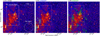 |
Fig. 1 Soft X-ray emission (0.2–0.5 keV) toward the N11 region observed with eROSITA. The white box and circle in (a) show the source and background regions, respectively. Blue contours with blue-shaded regions in (b) and green contours with green-shaded regions in (c) show the spatial distributions of the HI L-component and the I-component, respectively. The dashed circle in (a) is the Bubble region used in the analysis. |
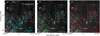 |
Fig. 2 Soft X-ray emission (0.2–0.6 keV) toward the northwestern part of the LMC, including the N11 region. eRASS1 map of Data Release 1 (DR1) is overlaid with HI (a) L-component (cyan), (b) I-component, and (c) D-component. The white box shows the analysis region of N11. |
2 Data sets
2.1 X-ray
In this paper, we used the X-ray data obtained with eROSITA. eROSITA was launched on July 13, 2019, on board the Spektrum-Roentgen-Gamma (Spektr-RG, SRG) spacecraft. It takes six months for one eROSITA All-Sky Survey (eRASS). The angular resolution averaged over the field of view is about 26″ (Predehl et al. 2021). We obtained the data set of the LMC by combining the four all-sky surveys eRASS1 to eRASS4 (hereafter referred to as eRASS: (4) executed between May 2020 and November 2021. The total exposure time of eRASS4:data ranges from around 9 to 17 ks toward the N11 region, which extends around 4º × 4º. To merge the data in the c020 processing version from all seven telescope, we used the evtool task of the eSASSusers_211214 (Brunner et al. 2022). Before extraction of spectra, we applied the recommended flag 0xc00f7f30 and pattern (15) filter keywords shown in the eSASS cookbook1.
2.2 HI
We used archival data of the HI 21 cm line emission of the whole LMC obtained with the Australia Telescope Compact Array (ATCA) and the Parkes telescope (Kim et al. 2003)2. The HI data obtained with ATCA (Kim et al. 1998) is combined with those obtained with the Parkes multibeam receiver with a resolution of 14′–16′ (Staveley-Smith et al. 1996, 2003). The angular resolution of the combined HI data is 60″ (corresponding to ~15 pc at the distance of the LMC). The root-mean-square (RMS) noise level is 2.4 K at a velocity resolution of 1.649 km s−1. More detailed descriptions of the observations are given by Kim et al. (2003).
2.3 CO
We used 12CO(J = 1–0) data of the MAGMA survey (Wong et al. 2011) to trace the H2 column density in each star-forming region3. The angular resolution was 45″ (corresponding to 11 pc at the distance of the LMC), and the velocity resolution was 0.526 km s−1. The MAGMA survey does not cover the whole LMC, and the observed area is limited to the individual CO clouds detected by the NANTEN survey.
We also used the latest ALMA 12CO(J = 2−1) data for a detailed investigation of the spatial distributions of the molecular clouds. The observation of N11 is a part of the ACA survey toward N11, N44, and N79 (project code 2019.2.00072.S and 2021.1.00490.S, PI: K. Tsuge). The target molecular lines were 12CO(J = 2−1), 13CO(J = 2−1), and C18O(J = 2−1). We used 12CO(J = 2−1) data as a tracer of the morphology of the total amount of the molecular clouds. The typical beam size is ~7.3″ × 6.6″ (~1.7 pc) and the RMS noise level is ~2 mK. Details of the observations, reductions, the results of other molecular lines, and the basic physical properties of the molecular clouds, are summarized in an overview paper currently in preparation (Tsuge et al., in prep.).
2.4 Optical
We also used optical images of the Magellanic Clouds Emission Lines Survey (MCELS) in Hα at 6563 Å, SII at 6275 Å, and [OIII] at 5007 Å taken with the Curtis Schmidt Telescope of the Cerro Tololo inter-American Observatory (CTiO; Smith et al. 2005). We mainly use optical images for the comparison of spatial distributions between star-forming regions and X-ray emission to investigate the origin of the diffuse X-rays.
3 Analysis
3.1 Calculation of NH from HI and CO
The diffuse X-ray emissions spread across a kpc scale and exhibit enhancement and depression of intensities as shown in Fig. 1. Understanding the characteristics of this X-ray emission requires comparing it with HI and CO gas. We calculated the total hydrogen column density NH,radio from HI and CO data. NH,radio is calculated as
 (1)
(1)
where NHI and  are the HI and H2 column densities, respectively. The NHI is calculated from the HI integrated intensity using a conversion factor of XHI = 1.82 × 10¹⁸/(K km s−1) (Dickey & Lockman 1990). The
  is estimated using the relationship
  between the hydrogen molecule column density
  and the 12CO(J = 1–0) integrated intensity W(CO) from Fukui et al. (2008).
3.2 X-ray
3.2.1 Imaging
eROSITA data were analyzed using the eSASS version eSASSusers_211214 (Brunner et al. 2022). We created exposure-time corrected images with the expmap task in the following bands: 0.2–0.5 keV, 0.5–0.7 keV, 0.5–1.0 keV, 0.7–1.0 keV, and 1.0–2.0 keV. TM1–TM7 imaging data were binned with a bin size of 160 pixels, yielding counts images with a pixel size of 8″. These counts images and corresponding exposure maps were created for each observation and energy band. We combined the image and exposure map into large mosaics by using evtool. The count maps were divided by the respective exposure map to create exposure-corrected images. Figure 1 shows the mosaic rate images in the energy band of0.2–0.5 keV. In the next step, we removed all point sources from the event file of each observation. For this purpose, we used the eRASS:4 point source catalog. The catalog contains the sources detected in the eRASS:4 data and was produced with pipeline version c020 (Merloni et al. 2024). The point sources are detected simultaneously in the three energy bands (1: 0.2–0.6 keV, 2: 0.6–2.3 keV, and 3: 2.3–5.0 keV). We used the sources detected in bands 1 and 2, which cover the energy range of the spectral fitting, to exclude them from the data for the spectral analysis of the diffuse emission. The typical size of a point source is 28″ (~2× half-energy width), and we manually adjust the size of point sources for very bright sources.
3.2.2 Extraction of spectra
We used srctool to extract spectra and response files for four regions: Dark lane region, Bubble region, Small region, and Diffuse region. For the response, we chose a sampling size of 5 pixels, which corresponds to ~40″. We defined one circle and three polygon regions based on the morphology of the soft X-ray emission. White lines in Fig. 3 indicate the four regions. The Dark lane region is a region where the soft X-ray emission is weaker than that of the surrounding region, as shown in Fig. 3b, and has a v-shaped structure. The Bubble region corresponds to the N11 super-bubble, which is one of the active star-forming regions. The Small region extends from the Bubble region to the north. The Diffuse region is extended over ~1 kpc in the southern part of N11. For TM5 and TM7 all data below 1.0 keV was ignored due to their contamination by optical light (Predehl et al. 2021). The spectra were binned to a minimum of 25 counts per bin.
4 Results
4.1 Spectral fit results
The spectra were analyzed using XSPEC version 12.12.1 (Arnaud 1996).
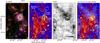 |
Fig. 3 Spatial distribution of multiwavelength emissions within the N11 analysis region highlighted by white squares in Figs. 2 and 1. (a) Optical three-color image with Hα (red), [SII] (green), and [OIII] (blue) (Smith et al. 2005). (b) Soft X-ray emission (0.2–0.5 keV) toward the N11 source region. White lines show the four extraction regions of the spectra. Black crosses and asterisks are O-type stars and WR stars (Bonanos et al. 2009), respectively. (c) Spatial distribution of the total hydrogen column density NH. The contour levels are 1.5 × 10²¹, 3.0 × 10²¹, 4.5 × 10²¹, and 6.0 × 1021 cm−2. The white box indicates the region shown in Fig. 7. (d) The total hydrogen column density map by contours superposed on soft X-ray emission (0.2–0.5 keV). |
4.1.1 Background components
To study the diffuse X-ray emission, we need to estimate and model the background component. We select a circular region with a radius of 30′ where there is only faint emission to measure the local background as shown in Fig. 1. The observation date, time, and exposure time of the eRASS scans vary across different regions, which implies that the intensity of emission produced by solar wind charge exchange (SWCX) possibly varies between regions. Therefore, we can not easily subtract the background (BG) spectrum directly from the spectrum of the source region. The background emission consists of the astrophysical X-ray background and the particle background.
Particle background. We used the model based on filter wheel closed (FWC) data obtained in the calibration and performance verification phase of eROSITA. The particle background consists of a continuum component that can be described with a broken power law combined with an exponential cut-off to model the signal above ~1.0–2.0 keV with additional emission lines caused in the instrument. The model is described in the appendix of Yeung et al. (2023).
This model is not folded through the effective area of the detectors and requires diagonal response matrices. These models were added and linked for each spectrum and each TM individually.
Astrophysical X-ray background. The astrophysical X-ray background was modeled as a combination of emission from the Local Hot Bubble, the cold- and hot Galactic halo, the extragalactic X-ray background, and SWCX. The Local Hot Bubble (LHB) is modeled with an unabsorbed thermal emission with a temperature of kT = 0.1 keV (Liu et al. 2017). Bluem et al. (2022) reported the correct temperature for the current APEC model to be 0.084 keV. This value is consistent with that of Liu et al. (2017) within the error range.The cold and hot Galactic halo is described by two absorbed thermal emission components with temperatures of kT = 0.1 keV and kT = 0.3–0.7 keV, respectively (Nakashima et al. 2018).We fixed the Galactic absorption column density to the value from the HI map of Dickey & Lockman (1990) at the center of the N11 region. The HI contribution of the LMC has been excluded from this HI map. We used an absorbed power law with photon index Γ = 1.46 and with an initial normalization of 8.88 × 10⁻⁷ cm−5 to model the unresolved extragalactic X-ray background (Kuntz & Snowden 2008; Snowden et al. 2008).This normalization, normalized to arcmin2, equals to 10.5 photons keV cm−2 s−1 sr−1. Finally, we accounted for SWCX emission using Gaussians at the position of the lines: 0.31 keV, CVI (0.46 keV), OVII (0.57 keV), OVIII (0.65 keV), OVIII (0.81 keV), NeIX (0.92 keV), and NeIX (1.02 keV) (Snowden et al. 2004). The model is described by Normalization between the TMs× skyarea×(SWCX lines + Local bubble + instrumental lines + Gal.abs ×(hot halo + cold halo + absorbed extragal. background), which is translated to the XSPEC model constant×constant×(multiple gaussians + apec + multiple gaussians + TBabs ×(apec + apec + TBvarabs×powerlaw)). The two constant values account for the normalization of the different TMs and the area normalization in arcmin−2, respectively. The normalization parameters of the model components are thus independent of the area.
The best-fit model agreed well with the data with a reduced χ2 of 600.64/654 = 0.92. The normalization of the local hot bubble thermal component is 4.62 × 10⁻¹¹ to 7.37 × 10⁻⁷ cm−5 arcmin−2. For the cold Galactic halo we obtain (1.81–3.24) × 10−6 cm−5 arcmin−2 and for the hot Galactic halo (3.56–4.57) × 10−7 cm−5 arcmin−2 and a temperature of kT = 0.25 keV. The background spectra with the best-fit model are shown in Fig. A.1. We applied the fitting results from the background region to constrain the background parameters of the N11 spectra. We used the 90% confidence range for the spectral fitting.
Spectral fit parameters of the manually selected four regions.
4.1.2 Model for N11 region
The results of the spectral analyses of the four selected regions are presented in the following subsections. We expect that extended emission from the hot ISM is dominated by two thermal components from previous analyses of the diffuse X-ray (e.g., Sasaki et al. 2022; Knies et al. 2021). Thus, we first tried the thermal plasma with the Galactic absorption and the LMC foreground absorption; TBabs×TBvarabs×(vapec + vapec) model in collisional ionization equilibrium (CIE). We fixed the Galactic absorption column density to the value from the HI map of Dickey & Lockman (1990) of 4.21 × 1020 cm−2 at the center of the N11 region with solar metallicity (Z⊙). The initial abundances of the TB varabs and vapec models were fixed to 0.5 Z⊙ (Rolleston et al. 2002). The temperatures of the two vapec components were approximately fit at around 0.2 keV and 0.8 keV. NH,X–ray is the X-ray column density in the LMC. We also applied a nonequilibrium ionization (NEI) model (vnei in XSPEC, Borkowski et al. 2001) instead of the hotter vapec component if we obtained a good fit. We constrained the ionization timescale (τ) of the hot plasma to investigate the time that had passed since the heating. The extended diffuse emission is faint and N11 has weaker emission compared to the stellar bar regions or the 30 Doradus region studied by Knies et al. (2021) or Sasaki et al. (2022), respectively. Thus, we did not conduct more complex models with variable abundances.
Dark lane region. We fitted the extended emission with the absorbed two-vapec model, which yielded kT = 0.15–0.18 keV and kT = 0.80–1.62 keV with NH,X–ray = (2.13–4.63) × 1021 cm−2 giving χ2/d.o.f. = 0.99 (see Table 1 and Fig. 4, top left). NH,radio is ~2.80 × 1021 cm−2 from HI and CO data.
Bubble region. The Bubble region was also well fitted with an absorbed two-vapec model yielding kT = 0.20–0.22 keV and kT = 0.79–0.96 keV with NH,X–ray = (1.56–2.83) × 1021 cm−2 giving χ2/d.o.f. = 1.06 (see Table 1 and Fig. 4, bottom left). NH,radio is ~3.47 × 1021 cm−2 from HI and CO data.
Small region. We fitted the spectra of the small region with absorbed two vapec model yielding kT = 0.20–0.22 keV and kT = 0.48–1.29 keV with NH,X–ray = (2.94–5.96) × 1021 cm−2 giving χ2/d.o.f. = 1.03 (see Table 1 and Fig. 4, upper right).
Diffuse region. The Diffuse region was well fitted with an absorbed two-vapec model with kT = 0.19–0.21 keV and kT = 0.70 – 0.81 keV with NH,X–ray = (0.17–0.50) × 1021 cm−2 giving χ2/d.o.f. = 1.06 (see Table 1 and Fig. 4, bottom left). NH,–radio is ~3.47 × 1021 cm−2 from HI and CO data. The temperature of vapec and vnei is kT = 0.21–0.23 keV and kT = 0.61–0.87 keV, respectively, which is consistent with the two-vapec model. The ionization time scale τ is (1.27–6.04) × 1011 s cm−3.
Nonequilibrium ionization (NEI) model. We also tried the vnei model instead of the hotter vapec component. The values of kT and τ are constrained toward the Bubble region and the Diffuse region. We could not constrain kT and tau toward the Small region and the Dark lane region. As for the Diffuse region, the temperature of vapec and vnei is kT = 0.21–0.23 keV and kT = 0.61–0.87 keV, respectively, which is consistent with the two-vapec model. The ionization timescale τ is (1.27–6.04) × 1011 s cm−3 and is thus consistent with the maximum timescales for most of the elements from Fig. 1 of Smith & Hughes (2010). Therefore, the Diffuse region could be considered close to collisional ionization equilibrium (CIE).
As for the Bubble region, the temperature of vapec and vnei is kT = 0.20–0.22 keV and kT= 0.77–0.98 keV, respectively, which is again consistent with the two-vapec model. The ion-ization timescale τ is (0.79–2.78) × 1011 s cm−3. This value of τ agrees with the maximum timescales for less heavy elements C, N, O, and Ne, also suggesting that it is near CIE.
We created contour plots for the Diffuse and Bubble regions showing the correlation between kT and τ (Fig. B.1). As can be seen, kT and τ are both well constrained in both regions.
4.2 Physical properties of the X-ray emitting hot plasma
We estimated the physical properties of the plasma, which emits the diffuse X-ray emission from the results of the spectral fitting. We limited the calculations to the hotter component, which most likely corresponds to the emission from plasma heated by the massive stars in the N11 region.
We calculated the unabsorbed flux FX for each region for the hotter vapec component using the cflux model in XSPEC with a 90% confidence error calculated by the error command. We calculated the luminosity from the flux using the equation as follows:
 (2)
(2)
where DLMC is the distance of the LMC (50±1.3 kpc; Pietrzyński et al. 2013). We normalized Fx and Lx by the area of each region to obtain the surface flux  and brightness
  for the comparison between regions normalizing again should yield the total emission (which then depends on the volume).
The gas density can be determined from the vapec spectral model normalization (norm). norm is defined as below:
![Mathematical equation: ${\rm{norm }} = {{{{10}^{ - 14}}} \over {4\pi D_{{\rm{LMC}}}^2}}\int {{n_{\rm{e}}}} {n_{\rm{H}}}f{\rm{d}}V\left[ {{\rm{c}}{{\rm{m}}^{ - 5}}} \right]{\rm{,}}$](/articles/aa/full_html/2024/06/aa48083-23/aa48083-23-eq29.png) (3)
(3)
where ne is the electron density, nH is the hydrogen density, f and V are the filling factor and the volume of the X-ray emissions, respectively. We used the relation of ne ~ 1.21 nH for the metallicity of the LMC (Sasaki et al. 2011). The hydrogen density nH is described as below,
![Mathematical equation: ${n_{\rm{H}}} = \sqrt {{{4\pi D_{{\rm{LMC}}}^2{{10}^{14}}} \over {1.21V}}} {f^{ - 0.5}}\left[ {{\rm{c}}{{\rm{m}}^{ - 3}}} \right].$](/articles/aa/full_html/2024/06/aa48083-23/aa48083-23-eq30.png) (4)
(4)
The pressure in the gas can be estimated from the gas density and temperature by assuming an ideal gas as
![Mathematical equation: $P{\rm{/}}{k_{\rm{B}}} = 2.31{n_{\rm{H}}}{T_{\rm{X}}}\left[ {{\rm{c}}{{\rm{m}}^{ - 3}}{\rm{K}}} \right],$](/articles/aa/full_html/2024/06/aa48083-23/aa48083-23-eq31.png) (5)
(5)
where TX is the X-ray temperature determined in the spectral fitting and kB is the Boltzmann constant. We can estimate the thermal energy E contained in the plasma with
![Mathematical equation: $E = {3 \over 2}PV\,f[{\rm{erg}}].$](/articles/aa/full_html/2024/06/aa48083-23/aa48083-23-eq32.png) (6)
(6)
Finally, the mass of the plasma can be calculated by using
![Mathematical equation: $M = 2.31{n_{\rm{H}}}{m_{\rm{H}}}\mu V\,f[{\rm{g}}]$](/articles/aa/full_html/2024/06/aa48083-23/aa48083-23-eq33.png) (7)
(7)
with the mH and µ are the hydrogen mass and molecular weight of the ionized gas, respectively.
We used the results of spectral fitting of the four regions for the calculations. The derived values are summarized in Table 2. We give the results without assuming any specific filling factor f. The volume V was estimated based on the morphology of each region. The area of the region is given by πr2, where r is the radius, assuming a circle. We assumed the depth of the region with z = 2r and the volume V is described πr2 × z. The assumed depth z of the dark lane, bubble, small, and diffuse regions are ~500, ~300, ~200, and ~530 pc, respectively.
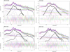 |
Fig. 4 Spectra of four regions: in the dark lane region (upper left), the small region (upper right), the diffuse region (lower left), and inside of the N11 bubble (lower right). Spectra of all TMs are shown in different colors. The source components are highlighted with thick lines (solid: lower-temperature vapec1; dashed: higher-temperature vapec2). The straight lines show the particle background. The thin dotted lines indicate the spectral components of the astrophysical background spectrum. |
4.3 Spatial distributions of the multiple phase ISM
4.3.1 X-rays
The spatial distributions of X-ray emission in the four energy bands of 0.2–0.5 keV, 0.5–0.7 keV, 0.7–1.0 keV, and 1.0–2.0 keV are shown in Fig. 5. The characteristics of each of the four analyzed regions in Fig. 3b are summarized as follows.
In the Dark lane region, the X-ray emission is weak in all energy bands while there is bright X-ray emission in the Bubble region in all energy ranges, as shown in Fig. 5. The harder emissions (0.7−1.0 keV; Fig. 5c) within the bubble exhibits a shell-like appearance. The emissions likely originate from locations where the ISM is heated by stellar winds. It is most likely enhanced where the stellar winds hits the shell of the bubble. In the Small region, there is diffuse X-ray emission in the energy ranges between 0.2 keV and 1.0 keV as shown in Fig. 5a. The diffuse X-ray emission extends over more than 500 pc toward the southwest, where the Diffuse region is located. The X-ray emissions in the lower energy bands of 0.2–0.5 keV and 0.5–0.7 keV are bright in the Diffuse region, while the emission appears weaker in the higher energy range (0.7–1.0 keV and 1.0–2.0 keV).
Physical properties of the diffuse X-ray emission (hot apec component).
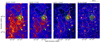 |
Fig. 5 Spatial distributions of X-ray emissions in the energy range of (a) 0.2–0.5 keV, (b) 0.5–0.7 keV, (c) 0.7–1.0 keV, and (d) 1.0–2.0 keV. White lines show the four extraction regions of the spectra. The green-shaded regions show the spatial distributions of Hα emission. |
4.3.2 Hα vs. X-rays
We compared the spatial distributions of Hα, high-mass stars, and X-ray emission. The Hα emissions mostly correspond to the distribution of high-mass stars. Most Hα emissions are distributed in the Bubble region as shown in Fig. 5. The Hα emission is also found in the Dark lane region and the Small region, but it is a minor component. These HII regions in the Dark lane region are likely located in front of the HI components.
In the Diffuse region, there is no Hα emission and no high-mass stars.
4.3.3 HI and CO vs. X-rays
Figure 3c shows the spatial distribution of the total hydrogen column density (NH) calculated from HI and CO. The details of the calculation are discussed in Sect. 3.1. NH is distributed in a v-shape toward the Dark lane region, Small region, and Bubble region. Mean NH values of the Dark lane region, Bubble region, and Small region are 2.80 × 10²¹, 3.47 × 10²¹, and 2.61 × 1021 cm−2, respectively as shown in Table 2. In the Diffuse region, hydrogen gas is faint, and NH is 0.90 × 1021 cm−2, less than one-third of other regions. Figure 3d shows the overlay of NH and soft X-ray. NH and soft X-ray show a nice anti-correlated spatial distribution in the Dark lane region.
Figures 6b, c, and d show the three velocity HI components of the L-, I-, and D-components, respectively. These components are defined by Fukui et al. (2017) and Tsuge et al. (2019). The integration ranges are Voffset: −100.1 to −30.5 km s−1 for the L-component; and Voffset: −30.5 to −10.4 km s−1 for the I-component; Voffset: −10.4 − 9.7 km s−1 for the D-component. We defined Voffset as a relative velocity from the rotational velocity of the D-component (Voffset = VLSR–VD; VD = the projected rotation velocity of the D-component). VD = 278 km s−1 at the position of N11. In the Bubble region, we observe emission of the L-component, but with low intensity. The I- and D-components are distributed in a v-shape toward the Dark lane region, Small region, and the Bubble region similar to NH. In the center of the Bubble region, the D-component is most likely ionized by highmass stars, which leads to a reduced intensity. The I-component is weaker than the D-component, but it extends over the entire Bubble region. The I- and D-components of the Diffuse region are very faint as shown in Figs. 6c and d.
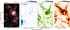 |
Fig. 6 The spatial distributions of optical emission and the three velocity HI components. (a) Optical three-color image with Hα (red), SII (green), and [OIII] (blue). The HI integrated intensity maps of (b) the L-component, (c) the I-component, and (d) the D-component. White lines and black dashed lines show the four extraction regions of the spectra. The integration ranges are VoffSet: −100.1 to −30.5 km s−1 for the L-component (b); and Voffset: −30.5 to −10.4 km s−1 for the I-component (c); Voffset: −10.4 to 9.7 km s−1 for the D-component (d). |
5 Discussion
5.1 Geometry of the ISM
There are two velocity components in the HI gas, the L-, D-, and I-components. In the N11 region, the intensity of the L component is weak. The velocity of the collision is 30–50 km s−1. Tsuge et al. (2024) have found observational signatures of gas collision between these two components as shown in the introduction. Figures 6b–d show the spatial distributions of the L-, I-,and D-components, respectively. In this section, we discuss the geometry of these components, which is important for the understanding of the heating mechanisms. Especially, we compared the X-ray absorption in the LMC from the fits (NH,X–ray) with the hydrogen column density calculated using HI and CO in only the velocity component of the LMC (NH,radio). Table 1 summarizes the NH,X–ray and the NH,radio.
5.1.1 Dark lane region
The HI and X-ray emissions show anti-correlated spatial distribution as shown in Fig. 3d. This trend suggests that the diffuse X-ray emission is absorbed by the cold ISM (HI and CO). NH,radio and NH,X–ray are consistent within the error range, as shown in Sect. 4.3.1 and Table 1.
5.1.2 Small region
NH,X–ray and NH,radio are almost same. Thus, the D- and I-components are located in front of the X-ray emission in the same way as in the Dark lane region. The X-ray emission of the small region is brighter than that of the dark lane region.
5.1.3 Diffuse region
As shown in Figs. 3c and 6, the intensity of NH,radio is weak in the Diffuse region, and there is a distribution of the faint D-component and the I-component. The NH,X–ray is smaller than NH,radio, indicating weak absorption and a lack of gas in the foreground.
5.1.4 Bubble region
NH,X–ray is smaller than NH,radio. This suggests that the cold ISM (HI, CO) exist both in front of and behind the X-ray emission. Furuta et al. (2021) also discussed a 3D geometry of the HI gas toward the Bubble region based on the comparison of Av and NH. The results suggest that the L-component has not yet fully penetrated through the D-component. The values of NH,X–ray, NH,radio(I), and NH,radio(D) are ~2.11 × 10²¹, 0.95 × 10²¹, and 2.30 × 1021 cm−2, respectively. NH,X–ray is roughly the same as NH,radio(D). Thus, it can possibly be interpreted that the X-ray emission is located between the L- and D-components during the collision.
In addition, we also compared the spatial distributions of the ALMA CO data and the X-ray emission toward the Bubble region. Figure 7 shows the spatial distributions of CO clouds, which have the same velocity as the HI D-component. The CO clouds are located at the edge of the superbubble in the optical image in Fig. 7a. We focused on this Bubble region and compared the spatial distributions of ALMA CO data and X-rays. Figures 7b and c show soft band (0.5–0.7 keV) and hard band (1.0–2.0 keV) X-ray distributions overlaid with ALMA CO, respectively. The soft band shows anti-correlated spatial distribution with CO, and the hard band X-ray is compact and its relation to the molecular cloud is unclear. Especially, in the northern part of the optical shell, the spatial distribution of hard X-ray and ALMA CO cloud are similar as shown in the yellow box of Fig. 7c, while that of the molecular cloud shows the same anti-correlated spatial distributions as in the soft band image (Fig. 7b). These trends suggest that some soft X-rays are absorbed by the dense molecular clouds on a small scale (<100 pc).
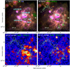 |
Fig. 7 Multiwavelength emissions toward the Bubble region of N11 by ALMA and eROSITA. (a) Optical image with Hα (red), SII (green), and [OIII] (blue). (b) Spatial distributions of ALMA12CO (J = 2−1) in green overlaid with the optical image. The spatial distribution of X-ray emissions with a velocity range of (c) 0.5–0.7 keV and (d) 1.0–2.0 keV. The green circle is SNR N11L (Maggi et al. 2016). No other SNR is observed by the latest ASKAP radio data in the whole region (Bozzetto et al. 2023). The black crosses and asterisks are O-type stars and WR stars (Bonanos et al. 2009), respectively. The boxes in (b), (c), and (d) represent the observation areas of ALMA, with the yellow discussed in Sect. 5.1.4. |
5.2 Energy input into the ISM
To constrain the origin of the diffuse X-ray emission, we compared the energy input of the stellar population into the ISM, the kinetic energy of HI gas, with the results derived from the spectral fitting.
We used a catalog of massive stars compiled from the literature (Bonanos et al. 2009). The authors catalogued 1750 high-mass stars having accurate coordinates and spectral classifications. The catalogue included the latest largest studies (see Table 1 of Bonanos et al. 2009).
Bubble region. The HII region N11 was catalogued by Henize (1956). N11 has a ring morphology with a cavity of ~100 pc in radius, enclosing OB association LH9 in the center of the cavity (Lucke & Hodge 1970). There are several bright nebulae (LH10 (N11B), LH13 (N11C), N11F, and LH14 (N11E)) around LH9 as shown in the Hα image in Fig. 7. The massive compact cluster of LH9 dominates this OB association and has an age of ~3.5 Myr (Walborn et al. 1999). LH 10 is the brightest nebula and lies to the north of LH 9. LH 10 is the youngest OB association with an age of about 1 Myr. We estimated the heating time based on the best-fit values of τ and ne, derived from the analysis presented in Sect. 4.1.2. Specifically, we obtained τ = ne × t = (0.79 to −2.78) × 1011 s and n = 1.21nH = 0.30 × 10⁻³cm−3. Using these values, we calculated t to be ~(8–30) Myr. This timescale is about an order of magnitude larger the age of N11, which is estimated to be 1–3.5 Myr (e.g., Walborn et al. 1999). There are two possible reasons for the large value of τ: (i) a long heating time, and (ii) a high initial electron density. Considering the active star-forming nature of the Bubble region, it is reasonable to assume that condition (ii) is responsible for the high value of τ. Assuming that the initial value of ne was about an order of magnitude higher than the present value, the heating timescale is consistent with the age of the Bubble region.
As for the Bubble region, there is a detailed spectroscopic analysis using the Fibre Large Array Multi-Element Spectro-graph (FLAMES) at the Very Large Telescope (Evans et al. 2006). We used the wind velocity, mass loss rate, and age cataloged by Mokiem et al. (2007). Mokiem et al. (2007) conducted a detailed analysis of optical spectra of 28 O- and early B-type stars using automatic spectral fitting (Mokiem et al. 2005).
We summarize the properties of the high-mass stellar content of theN11 superbubble in Table 3 (see Tables 1 and 2, and Fig. 13 of Mokiem et al. 2007). Using these ages, mass loss rate, and wind velocities, we estimated that the O- and early B-type stars in the bubble region have supplied a total energy of (5.9±1.8) × 1051 erg and a mass of (100±30) M⊙. We also estimated the energy input of previous supernovae (SNe). We assumed that the stellar populations formed from the same parental molecular cloud and number of stars is described by a Salpeter initial mass function (IMF; Kroupa 2001). From the Hertzsprung-Russell diagram from Fig. 12 of Mokiem et al. (2007), we find 15 stars in the 20–40 M⊙ bins and 5 stars with masses >40 M⊙. Using the number of 15, we estimated the number of stars above 40 M⊙ from  . We found that the number of observed stars is short by 1–3. Thus, we estimate that (2±1) SN have already occurred in the N11 bubble. Assuming an SN explosion energy of 1051 erg, these SNe have ejected ~(2±1) × 1051 erg, and assuming an average initial mass of 60 M⊙, they supplied (120±60) M⊙ of material. Thus, total Estellar and energy density ρstellar are (5.8–10.0) × 1051 erg and (9.1–15.7) × 10−12 erg cm−3, respectively.
As for other regions, we applied 3±1 Myr which is the same timescale as LH10 The total stellar mass was estimated by assuming the Salpeter IMF (Kroupa 2001). We used the number of stars in the 20–30 M⊙, and adopt α = 2.37 for Mstar > 0.5 M⊙ and α = 1.37 for Mstar ≤ 0.5 M⊙. We obtained the stellar energy input by using the Starburst99 code (Leitherer et al. 1999; Leitherer & Chen 2009). The simulations take into account both the energy input by supernova remnants (SNRs) and stellar winds into the ISM. As inputs, we use the total stellar mass assuming IMF and assume a metallicity of 0.5 Z⊙. The values of total stellar mass for each region are specified in respective sections.
Dark lane region. We estimated the total stellar mass of the dark lane region as ~2000 M⊙ assuming the IMF. Using the star-burst 99 simulations, we estimated ~1 SN has occurred, and the injected Energy Estellar and energy density ρstellar by stars and SNe are ~(1.3–3.6) × 1051 erg and (0.6–0.7) × 10−12 erg cm−3, respectively.
Small region. The total stellar mass based on the IMF function is ~300 M⊙. We estimated ~1 SN has occurred, and the energy input Estellar and an energy density ρstellar are (0.6–1.8) × 1051 erg and (4.4–5.5) × 10−12 erg cm−3, respectively.
Diffuse region. In the Diffuse region, there are no catalogued high-mass stars, and the current star formation is inactive, and it is difficult to estimate the energy input from the number of high-mass stars. Thus, we used the past star-forming activities by optical/near-infrared studies. The previous optical/near-infrared observations (Harris & Zaritsky 2009, HZ09; Mazzi et al. 2021, M21) revealed star formation histories (SFHs) for the entire LMC. HZ09 and M21 are based on the optical observation (U, B, V, and I band) from the Magellanic Clouds Photometric Survey (MCPS) and near-infrared observation (J, Y, and Ks band) from the VISTA survey (Cioni et al. 2011), respectively. Optical observation (HZ09) possibly provides a better color separation for young stars. While M21 covers about 50% larger area than that obtained from the optical data by HZ09. The time evolution of star formation rate (SFR) is plotted for four regions. The trends of HZ09 and M21 are consistent for t < 108 yr in all regions We estimated the total stellar mass of the most recent star formation peak. The results of HZ09 and M 21 are consistent within 108 yr. We applied the result of HZ09, which allows a better separation of young stars. The calculated total stellar mass is ~915 M⊙ by assuming a constant star formation rate for the given time interval. Using the starburst 99 simulations, we estimated ~1 SN has occurred, and the injected Energy Estellar and energy density ρstellar by stars and SNe are ~(1.3–3.6) × 1051 erg and (0.5–0.6) × 10−12 erg cm−3, respectively. The timescale 108 yr used to estimate the energy input from past star formation activity is consistent with the heating timescale estimated from the ionization timescale τ obtained by the vnei model. As in the Bubble region, the value of the τ~(1.27–6.04)× 1011 s, ne = 0.07 × 10⁻³, as shown in Sect. 4.1.2, gives t ~ (55–260) Myr. From these results, it is considered that this region was under condition i) and may have been heated for a long time.
Total energy of hot plasma and stellar energy input.
5.3 Kinetic energy of HI gases
We also estimated the kinetic energy of HI gas collision (EHI) of each region from  MHI
MHI . As suggested by Tsuge et al. (2020), there the compressed region due to gas collision is possibly traced by the I-component. Thus, the HI mass of the I-component (MHI) and the collision velocity of 30 km s−1 are used for the calculation. The estimated kinetic energy is on the order of several 1051 erg as shown in Table 3. The estimation is based on the assumption that HI collision occurred in all regions. Observational evidence of HI collision is found in the Dark lane, Small, and Bubble regions (Tsuge et al. 2019, Tsuge et al. 2020). However, in the Diffuse region, HI gas is very weak, and it is difficult to verify the observational evidence of the collision. However, the diffuse I-and D-components in the Diffuse region indicate the possibility of the past HI collision.
5.4 Origin of the diffuse X-rays
We discuss the origin of diffuse X-rays by comparing the estimations of Sects. 5.2.1–5.2.3. The estimations of energy input are summarized in Table 3. We should assume the value of the filling factor for the discussion. For a young stellar bubble, the filling parameter is likely f ~ 1 (see Oey & García-Segura 2004; Sasaki et al. 2011, for example). Hence, we adopt f = 1 for the Bubble region. As for the other regions, we also used f = 1.0 assuming that the gas is well mixed and relaxed, and discussed the energy input.
The low-temperature component (~0.2 keV, apec) extends throughout the LMC (Snowden 1998), while locally, a two-temperature component model (around 0.2 keV and 0.6 keV) better reproduces the emission from thermal plasma (Knies et al. 2021; Sasaki et al. 2022, and references therein). We mainly focus on the high-temperature component to examine the potential heating from recent star formation or gas collisions.
Dark lane region. The plasma energies Ep at f = 1.0 is ~(0.95–1.99) × 1051 erg. The energy input by star formation Estellar and the kinetic energy of HI gas EHI are ~(1.3–3.6) × 1051 erg and ~5 × 1051 erg, respectively. Estellar, Ep, and EHI are roughly comparable. The sum of Estellar and EHI are larger than Ep, and it is sufficient to explain the plasma energy Ep of 1.26 × 1051 erg if the efficiency of the stellar winds injection into the ISM is ~20 % (Weaver et al. 1977).
Small region. The plasma energies Ep at f = 1.0 is (0.46–1.05) × 1051 erg. In this region, the energy input of high-mass stars Estellar ~ Ep ~ EHI. In this region, HI collision is confirmed as in the Dark lane region, and the kinetic energy is ~2 × 1051 erg. If the efficiency of the stellar winds injection into the ISM is ~20% (Weaver et al. 1977), neither stellar energy input nor HI gas collision can explain the X-ray energy. The diffuse emission is nicely anticorrelated with the HI D component. Therefore, it is likely there is outflow of plasma from the Bubble region along the cavity seen in HI.
Diffuse region. This region is very faint in both optical observations, HI, and CO. Thus, it is difficult to investigate the origin of the X-ray emissions. The plasma energies Ep at f= 1.0 is ~(1.53–1.74) × 1051 erg. The stellar energy input Estellar and the HI kinetic energy (EHI) are ~(1.3–3.6) × 1051 erg and ~2.0 × 1051 erg, respectively, which are sufficient to explain the energy of X-rays. The sum of Estellar and EHI can explain the energy of the plasma, even if injection efficiency is ~20%.
Bubble region. The plasma energies Ep at f = 1.0 is ~1.42 × 1051 erg. There are 30 high-mass stars in the Bubble region, and a stellar energy input Estellar of ~(5.8–10.0) × 1051 erg is expected. The energy balance is Estellar = Ep +EHI, and the diffuse X-rays are heated by the stellar energy input. Moreover, it is likely that the dynamics of the HI I-component is locally affected by the stellar feedback.
We compared the results of normalization values of the hotter component (norm2) from Table 1. The normalization of the fitting model is scaled by the area of the region, making it directly comparable. The bubble region and diffuse region in the N11 region, similar to the northern part of the Dark lane, lack absorption by hydrogen gas, but the hot components of the Bubble and Diffuse regions are more than an order of magnitude stronger than that of the Small and Dark lane regions. The strength of the emission in terms of norm2 values varies as Dark lane ≪ Small ~ Bubble < Diffuse. Therefore, no apparent differences based on the distance from the bubble are observed. In the future, comparing results from multiple locations across the entire LMC will allow for a comprehensive investigation of critical physical quantities involved in gas heating.
6 Conclusions
We analyzed the diffuse X-ray emission in the LMC’s N11 region using data obtained with eROSITA in the surveys eRASS1–4. We focused on diffuse X-ray emission by excluding all point and point-like sources. We divided the data into four regions (Dark lane, Small, Diffuse, and Bubble regions) based on the morphology of the X-ray emission. We derived physical parameters of plasma from X-ray spectral fitting toward these four regions and compared them with HI and CO data. The X-ray emission in the four regions is well-fitted with an absorbed model consisting of thermal plasma models. The absorption by HI and CO clouds causes the X-ray dark lane region. By estimating the energy budget of the thermal plasma, the energy of the Bubble region can be explained by heating by high-mass stars. The energy of the X-ray emission of the other regions can be explained by stellar feedback with possible contribution from large-scale HI colli-sions. The main conclusions of the present paper are summarized as follows:
The X-ray emissions in the four regions were fitted by absorbed two thermal CIE plasma model with kT = ~0.2 keV and kT = ~0.8–1.0 keV.
The absorption column densities from X-ray fitting (NH,X–ray) of the Dark lane, Small, Diffuse, and Bubble regions are 3.13, 2.10, 4.07, and 0.35 × 1021 cm−2, respectively. The total hydrogen column density from HI and CO (NH,radio) of the Dark lane, Small, Diffuse, and Bubble regions are 2.80, 3.47, 2.61, and 0.90 × 1021 cm−2, respectively.
As for the Bubble region and the Diffuse region, the hotter CIE component was also fitted well with a NEI model. The temperature of the lower-temperature CIE component and the absorption column density are consistent with those of the two-CIE model.
Dark lane and Small regions: NH,X–ray ~ NH,radio. The diffuse X-ray is absorbed by the cold ISM, and the Dark lane region was formed by absorption.
Diffuse region: NH,X–ray and NH,radio are less than 1021 cm−2, and the absorption is weak in this region.
Bubble region: NH,X–ray < NH,radio. The cold ISM (HI and CO) partially absorbed X-rays. One possible scenario is that the X-ray emission is located between the I- and D-components during the collision.
The estimation of  for the absorption has uncertainties due to the uncertainty of the CO-to-H2 conversion factor (Bolatto et al. 2013). Most of the CO is distributed in the Bubble region and the Dark lane region. Even if the values in these regions vary by a factor of 2, the conclusions remain unchanged. Additionally, systematic offsets in the X-ray values are possible, so a more detailed evaluation of absolute values is future work.
4. Based on the estimation of the energy budget of the plasma, the heating mechanism of the X-rays is discussed. We estimated the energy input by stars (Estellar) and the kinetic energy of HI gas (EHI), and compared it with the energy of the plasma gas (Ep).
Dark lane region: Estellar ~ Ep < EHI. Estellar is insufficient for heating of the plasma to explain the X-ray luminosity. The combination of Estellar and EHI is sufficient to explain Ep even if the efficiency is ~10–20 % considering the solid angle of energy input.
Small region: Estellar ~ Ep ~ EHI. Assuming an injection efficiency of 20%, the stellar input is insufficient. The emission is likely due to plasma heated in by the stars in the Bubble region, escaping into a cavity in the HI distribution at the position of the Small region.
Diffuse region: Estellar ~ Ep ~ EHI. It is difficult to distinguish between heating by star formation and heating due to, e.g., gas collision. The estimation of the energy budget suggests that the combination of Estellar and EHI is sufficient to explain Ep.
Bubble region: Ep = Estellar + EHI. The diffuse X-rays are heated by the stellar energy input and the dynamics of HI gas is affected by stellar feedback.
Acknowledgements
This work is based on data from eROSITA, the soft X-ray instrument aboard SRG, a joint Russian-German science mission supported by the Russian Space Agency (Roskosmos), in the interests of the Russian Academy of Sciences represented by its Space Research Institute (IKI), and the Deutsches Zentrum für Luft- und Raumfahrt (DLR). The SRG spacecraft was built by Lav-ochkin Association (NPOL) and its subcontractors and is operated by NPOL with support from the Max Planck Institute for Extraterrestrial Physics (MPE). The development and construction of the eROSITA X-ray instrument was led by MPE, with contributions from the Dr. Karl Remeis Observatory Bamberg & ECAP (FAU Erlangen-Nürnberg), the University of Hamburg Observatory, the Leibniz Institute for Astrophysics Potsdam (AIP), and the Institute for Astronomy and Astrophysics of the University of Tübingen, with the support of DLR and the Max Planck Society. The Argelander Institute for Astronomy of the University of Bonn and the Ludwig Maximilians Universität Munich also participated in the science preparation for eROSITA. The eROSITA data shown here were processed using the eSASS software system developed by the German eROSITA consortium. This research has made use of data and/or software provided by the High Energy Astrophysics Science Archive Research Center (HEASARC), which is a service of the Astrophysics Science Division at NASA/GSFC and the High Energy Astrophysics Division of the Smithsonian Astrophysical Observatory. The ATCA, Parkes, and Mopra radio telescope are part of the ATNF, which is funded by the Australian Government for operation as a National Facility managed by CSIRO. The UNSW Digital Filter Bank used for the observations with the Mopra Telescope was provided with support from the Australian Research Council. The NANTEN project is based on a mutual agreement between Nagoya University and the Carnegie Institution of Washington (CIW). We greatly appreciate the hospitality of all the Las Campanas Observatory staff members of CIW. We are thankful to many Japanese public donors and companies who contributed to the realization of the project. This paper made use of the following ALMA data: ADS/JAO.ALMA#2019.2.00072.S and ADS/JAO.ALMA#2021.1.00490.S. ALMA is a partnership between ESO (representing its member states), NSF (USA) and NINS (Japan), together with NRC (Canada), MOST and ASIAA (Taiwan), and KASI (Republic of Korea), in cooperation with the Republic of Chile. The Joint ALMA Observatory is operated by ESO, AUI/NRAO and NAOJ. This research is based on support from the Deutsche Forschungsgemeinschaft through the grants SA 2131/13-1, SA 2131/14-1, and SA 2131/15-1.
Appendix A Background modeling
We present the fitting result of the background region. The details of the model and results are provided in Section 4.1.1
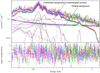 |
Fig. A.1 Spectra of the background region. Spectra of all TMs are shown in different colors. The straight lines represent the particle background. The Gaussians correspond to the SWCX lines and the detector line. The three thermal components consist of the hot halo, cold halo, and local hot bubble. The unresolved background of cosmological sources is fitted with an absorbed power-law model, with a photon index Γ = 1.46. |
Appendix B Correlation between kT and τ
We show the correlation plots between kT and τ of the Diffuse and Bubble regions to investigate the equilibrium problem as shown in Figure B.1. We calculated the confidence ranges of τ and kT using steppar command and plotted the contours. There was no clear anti-correlation in either of the two regions.
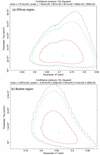 |
Fig. B.1 Contour plots showing the correlation between kT and τ in the Diffuse region (upper panel) and the inside of the N11 bubble (lower panel). The contour levels are Δχ2 = 1, 2.3, and 2.7. |
References
- Anathpindika, S. V. 2010, MNRAS, 405, 1431 [NASA ADS] [Google Scholar]
- Arnaud, K. A. 1996, ASP Conf. Ser., 101, 17 [Google Scholar]
- Blondiau, M. J., Kerp, J., Mebold, U., & Klein, U. 1997, A&A, 323, 585 [NASA ADS] [Google Scholar]
- Bluem, J., Kaaret, P., Kuntz, K. D., et al. 2022, ApJ, 936, 72 [NASA ADS] [CrossRef] [Google Scholar]
- Bolatto, A. D., Wolfire, M., & Leroy, A. K. 2013, ARA&A, 51, 207 [CrossRef] [Google Scholar]
- Bonanos, A. Z., Massa, D. L., Sewilo, M., et al. 2009, AJ, 138, 1003 [Google Scholar]
- Borkowski, K. J., Arnaud, K. A., Dorman, B., et al. 2001, AAS Meet. Abstr., 199, 126.19 [NASA ADS] [Google Scholar]
- Bozzetto, L. M., Filipović, M. D., Sano, H., et al. 2023, MNRAS, 518, 2574 [Google Scholar]
- Brunner, H., Liu, T., Lamer, G., et al. 2022, A&A, 661, A1 [NASA ADS] [CrossRef] [EDP Sciences] [Google Scholar]
- Chu, Y.-H., & Mac Low, M.-M. 1990, ApJ, 365, 510 [NASA ADS] [CrossRef] [Google Scholar]
- Cioni, M. R. L., Clementini, G., Girardi, L., et al. 2011, A&A, 527, A116 [CrossRef] [EDP Sciences] [Google Scholar]
- Dickey, J. M., & Lockman, F. J. 1990, ARA&A, 28, 215 [Google Scholar]
- Evans, C. J., Lennon, D. J., Smartt, S. J., & Trundle, C. 2006, A&A, 456, 623 [CrossRef] [EDP Sciences] [Google Scholar]
- Fabbiano, G., Krauss, M., Zezas, A., Rots, A., & Neff, S. 2003, ApJ, 598, 272 [NASA ADS] [CrossRef] [Google Scholar]
- Fukui, Y., Mizuno, N., Yamaguchi, R., et al. 1999, PASJ, 51, 745 [Google Scholar]
- Fukui, Y., Kawamura, A., Minamidani, T., et al. 2008, ApJS, 178, 56 [Google Scholar]
- Fukui, Y., Tsuge, K., Sano, H., et al. 2017, PASJ, 69, L5 [Google Scholar]
- Fukui, Y., Torii, K., Hattori, Y., et al. 2018, ApJ, 859, 166 [Google Scholar]
- Fukui, Y., Tokuda, K., Saigo, K., et al. 2019, ApJ, 886, 14 [NASA ADS] [CrossRef] [Google Scholar]
- Fukui, Y., Habe, A., Inoue, T., Enokiya, R., & Tachihara, K. 2021a, PASJ, 73, S1 [NASA ADS] [CrossRef] [Google Scholar]
- Fukui, Y., Inoue, T., Hayakawa, T., & Torii, K. 2021b, PASJ, 73, S405 [NASA ADS] [CrossRef] [Google Scholar]
- Furuta, T., Kaneda, H., Kokusho, T., et al. 2019, PASJ, 71, 95 [Google Scholar]
- Furuta, T., Kaneda, H., Kokusho, T., et al. 2021, PASJ, 73, 864 [NASA ADS] [CrossRef] [Google Scholar]
- Habe, A., & Ohta, K. 1992, PASJ, 44, 203 [NASA ADS] [Google Scholar]
- Harris, J., & Zaritsky, D. 2009, AJ, 138, 1243 [NASA ADS] [CrossRef] [Google Scholar]
- Henize, K. G. 1956, ApJS, 2, 315 [CrossRef] [Google Scholar]
- Inoue, T., Hennebelle, P., Fukui, Y., et al. 2018, PASJ, 70, S53 [NASA ADS] [Google Scholar]
- Kavanagh, P. J., Sasaki, M., Breitschwerdt, D., et al. 2020, A&A, 637, A12 [EDP Sciences] [Google Scholar]
- Kim, S., Staveley-Smith, L., Dopita, M. A., et al. 1998, ApJ, 503, 674 [Google Scholar]
- Kim, S., Staveley-Smith, L., Dopita, M. A., et al. 2003, ApJS, 148, 473 [Google Scholar]
- Knies, J. R., Sasaki, M., Fukui, Y., et al. 2021, A&A, 648, A90 [NASA ADS] [CrossRef] [EDP Sciences] [Google Scholar]
- Kobayashi, M. I. N., Kobayashi, H., Inutsuka, S.-I., & Fukui, Y. 2018, PASJ, 70, S59 [NASA ADS] [CrossRef] [Google Scholar]
- Kroupa, P. 2001, MNRAS, 322, 231 [NASA ADS] [CrossRef] [Google Scholar]
- Kuntz, K. D., & Snowden, S. L. 2008, ApJ, 674, 209 [NASA ADS] [CrossRef] [Google Scholar]
- Leitherer, C., & Chen, J. 2009, New A, 14, 356 [NASA ADS] [CrossRef] [Google Scholar]
- Leitherer, C., Schaerer, D., Goldader, J. D., et al. 1999, ApJS, 123, 3 [Google Scholar]
- Liu, W., Chiao, M., Collier, M. R., et al. 2017, ApJ, 834, 33 [Google Scholar]
- Lucke, P. B., & Hodge, P. W. 1970, AJ, 75, 171 [NASA ADS] [CrossRef] [Google Scholar]
- Luks, T., & Rohlfs, K. 1992, A&A, 263, 41 [NASA ADS] [Google Scholar]
- Maddox, L. A., Williams, R. M., Dunne, B. C., & Chu, Y. H. 2009, ApJ, 699, 911 [NASA ADS] [CrossRef] [Google Scholar]
- Maeda, R., Inoue, T., & Fukui, Y. 2021, ApJ, 908, 2 [NASA ADS] [CrossRef] [Google Scholar]
- Maggi, P., Haberl, F., Kavanagh, P. J., et al. 2016, A&A, 585, A162 [NASA ADS] [CrossRef] [EDP Sciences] [Google Scholar]
- Mazzi, A., Girardi, L., Zaggia, S., et al. 2021, MNRAS, 508, 245 [NASA ADS] [CrossRef] [Google Scholar]
- Meaburn, J. 1980, MNRAS, 192, 365 [NASA ADS] [CrossRef] [Google Scholar]
- Merloni, A., Predehl, P., Becker, W., et al. 2012, arXiv e-prints [arXiv:1209.3114] [Google Scholar]
- Merloni, A., Predehl, P., Becker, W., et al. 2024, A&A, 682, A34 [NASA ADS] [CrossRef] [EDP Sciences] [Google Scholar]
- Mizuno, N., Yamaguchi, R., Mizuno, A., et al. 2001, PASJ, 53, 971 [NASA ADS] [Google Scholar]
- Mokiem, M. R., de Koter, A., Puls, J., et al. 2005, A&A, 441, 711 [NASA ADS] [CrossRef] [EDP Sciences] [Google Scholar]
- Mokiem, M. R., de Koter, A., Evans, C. J., et al. 2007, A&A, 465, 1003 [NASA ADS] [CrossRef] [EDP Sciences] [Google Scholar]
- Nakashima, S., Inoue, Y., Yamasaki, N., et al. 2018, ApJ, 862, 34 [CrossRef] [Google Scholar]
- Nazé, Y., Antokhin, I. I., Rauw, G., et al. 2004, A&A, 418, 841 [NASA ADS] [CrossRef] [EDP Sciences] [Google Scholar]
- Oey, M. S., & García-Segura, G. 2004, ApJ, 613, 302 [NASA ADS] [CrossRef] [Google Scholar]
- Oh, S.-H., Kim, S., For, B.-Q., & Staveley-Smith, L. 2022, ApJ, 928, 177 [NASA ADS] [CrossRef] [Google Scholar]
- O’sullivan, E., Giacintucci, S., Vrtilek, J. M., Raychaudhury, S., & David, L. P. 2009, ApJ, 701, 1560 [CrossRef] [Google Scholar]
- Pietrzyński, G., Graczyk, D., Gieren, W., et al. 2013, Nature, 495, 76 [Google Scholar]
- Points, S. D., Chu, Y. H., Snowden, S. L., & Smith, R. C. 2001, ApJS, 136, 99 [NASA ADS] [CrossRef] [Google Scholar]
- Predehl, P., Andritschke, R., Arefiev, V., et al. 2021, A&A, 647, A1 [EDP Sciences] [Google Scholar]
- Rolleston, W. R. J., Trundle, C., & Dufton, P. L. 2002, A&A, 396, 53 [NASA ADS] [CrossRef] [EDP Sciences] [Google Scholar]
- Rosado, M., Laval, A., Le Coarer, E., et al. 1996, A&A, 308, 588 [NASA ADS] [Google Scholar]
- Sakre, N., Habe, A., Pettitt, A. R., & Okamoto, T. 2021, PASJ, 73, S385 [NASA ADS] [CrossRef] [Google Scholar]
- Sasaki, M., Haberl, F., & Pietsch, W. 2002, A&A, 392, 103 [NASA ADS] [CrossRef] [EDP Sciences] [Google Scholar]
- Sasaki, M., Breitschwerdt, D., Baumgartner, V., & Haberl, F. 2011, A&A, 528, A136 [NASA ADS] [CrossRef] [EDP Sciences] [Google Scholar]
- Sasaki, M., Knies, J., Haberl, F., et al. 2022, A&A, 661, A37 [NASA ADS] [CrossRef] [EDP Sciences] [Google Scholar]
- Shima, K., Tasker, E. J., Federrath, C., & Habe, A. 2018, PASJ, 70, S54 [Google Scholar]
- Smith, R. K., & Hughes, J. P. 2010, ApJ, 718, 583 [NASA ADS] [CrossRef] [Google Scholar]
- Smith, R. C., Points, S., Chu, Y. H., et al. 2005, AAS Meet. Abstr., 207, 145.01 [NASA ADS] [Google Scholar]
- Snowden, S. L. 1998, ASP Conf. Ser., 136, 127 [NASA ADS] [Google Scholar]
- Snowden, S. L., & Petre, R. 1994, ApJ, 436, L123 [NASA ADS] [CrossRef] [Google Scholar]
- Snowden, S. L., Collier, M. R., & Kuntz, K. D. 2004, ApJ, 610, 1182 [Google Scholar]
- Snowden, S. L., Mushotzky, R. F., Kuntz, K. D., & Davis, D. S. 2008, A&A, 478, 615 [NASA ADS] [CrossRef] [EDP Sciences] [Google Scholar]
- Staveley-Smith, L., Wilson, W. E., Bird, T. S., et al. 1996, PASA, 13, 243 [NASA ADS] [CrossRef] [Google Scholar]
- Staveley-Smith, L., Kim, S., Calabretta, M. R., Haynes, R. F., & Kesteven, M. J. 2003, MNRAS, 339, 87 [NASA ADS] [CrossRef] [Google Scholar]
- Subramanian, S., & Subramaniam, A. 2010, A&A, 520, A24 [NASA ADS] [CrossRef] [EDP Sciences] [Google Scholar]
- Takahira, K., Tasker, E. J., & Habe, A. 2014, ApJ, 792, 63 [Google Scholar]
- Takahira, K., Shima, K., Habe, A., & Tasker, E. J. 2018, PASJ, 70, S58 [Google Scholar]
- Tokuda, K., Fukui, Y., Harada, R., et al. 2019, ApJ, 886, 15 [NASA ADS] [CrossRef] [Google Scholar]
- Tsuge, K., Sano, H., Tachihara, K., et al. 2019, ApJ, 871, 44 [Google Scholar]
- Tsuge, K., Sano, H., Tachihara, K., et al. 2020, arXiv e-prints [arXiv:2010.08816] [Google Scholar]
- Tsuge, K., Sano, H., Tachihara, K., et al., 2024, PASJ, submitted [arXiv:2405.05046] [Google Scholar]
- Walborn, N. R., Drissen, L., Parker, J. W., et al. 1999, AJ, 118, 1684 [NASA ADS] [CrossRef] [Google Scholar]
- Wang, Q., Hamilton, T., Helfand, D. J., & Wu, X. 1991, ApJ, 374, 475 [NASA ADS] [CrossRef] [Google Scholar]
- Weaver, R., McCray, R., Castor, J., Shapiro, P., & Moore, R. 1977, ApJ, 218, 377 [Google Scholar]
- Wong, T., Hughes, A., Ott, J., et al. 2011, ApJS, 197, 16 [NASA ADS] [CrossRef] [Google Scholar]
- Yamaguchi, H., Sawada, M., & Bamba, A. 2010, ApJ, 715, 412 [NASA ADS] [CrossRef] [Google Scholar]
- Yeung, M. C. H., Freyberg, M. J., Ponti, G., et al. 2023, A&A, 676, A3 [NASA ADS] [CrossRef] [EDP Sciences] [Google Scholar]
All Tables
All Figures
|
Fig. 1 Soft X-ray emission (0.2–0.5 keV) toward the N11 region observed with eROSITA. The white box and circle in (a) show the source and background regions, respectively. Blue contours with blue-shaded regions in (b) and green contours with green-shaded regions in (c) show the spatial distributions of the HI L-component and the I-component, respectively. The dashed circle in (a) is the Bubble region used in the analysis. |
| In the text | |
|
Fig. 2 Soft X-ray emission (0.2–0.6 keV) toward the northwestern part of the LMC, including the N11 region. eRASS1 map of Data Release 1 (DR1) is overlaid with HI (a) L-component (cyan), (b) I-component, and (c) D-component. The white box shows the analysis region of N11. |
| In the text | |
|
Fig. 3 Spatial distribution of multiwavelength emissions within the N11 analysis region highlighted by white squares in Figs. 2 and 1. (a) Optical three-color image with Hα (red), [SII] (green), and [OIII] (blue) (Smith et al. 2005). (b) Soft X-ray emission (0.2–0.5 keV) toward the N11 source region. White lines show the four extraction regions of the spectra. Black crosses and asterisks are O-type stars and WR stars (Bonanos et al. 2009), respectively. (c) Spatial distribution of the total hydrogen column density NH. The contour levels are 1.5 × 10²¹, 3.0 × 10²¹, 4.5 × 10²¹, and 6.0 × 1021 cm−2. The white box indicates the region shown in Fig. 7. (d) The total hydrogen column density map by contours superposed on soft X-ray emission (0.2–0.5 keV). |
| In the text | |
|
Fig. 4 Spectra of four regions: in the dark lane region (upper left), the small region (upper right), the diffuse region (lower left), and inside of the N11 bubble (lower right). Spectra of all TMs are shown in different colors. The source components are highlighted with thick lines (solid: lower-temperature vapec1; dashed: higher-temperature vapec2). The straight lines show the particle background. The thin dotted lines indicate the spectral components of the astrophysical background spectrum. |
| In the text | |
|
Fig. 5 Spatial distributions of X-ray emissions in the energy range of (a) 0.2–0.5 keV, (b) 0.5–0.7 keV, (c) 0.7–1.0 keV, and (d) 1.0–2.0 keV. White lines show the four extraction regions of the spectra. The green-shaded regions show the spatial distributions of Hα emission. |
| In the text | |
|
Fig. 6 The spatial distributions of optical emission and the three velocity HI components. (a) Optical three-color image with Hα (red), SII (green), and [OIII] (blue). The HI integrated intensity maps of (b) the L-component, (c) the I-component, and (d) the D-component. White lines and black dashed lines show the four extraction regions of the spectra. The integration ranges are VoffSet: −100.1 to −30.5 km s−1 for the L-component (b); and Voffset: −30.5 to −10.4 km s−1 for the I-component (c); Voffset: −10.4 to 9.7 km s−1 for the D-component (d). |
| In the text | |
|
Fig. 7 Multiwavelength emissions toward the Bubble region of N11 by ALMA and eROSITA. (a) Optical image with Hα (red), SII (green), and [OIII] (blue). (b) Spatial distributions of ALMA12CO (J = 2−1) in green overlaid with the optical image. The spatial distribution of X-ray emissions with a velocity range of (c) 0.5–0.7 keV and (d) 1.0–2.0 keV. The green circle is SNR N11L (Maggi et al. 2016). No other SNR is observed by the latest ASKAP radio data in the whole region (Bozzetto et al. 2023). The black crosses and asterisks are O-type stars and WR stars (Bonanos et al. 2009), respectively. The boxes in (b), (c), and (d) represent the observation areas of ALMA, with the yellow discussed in Sect. 5.1.4. |
| In the text | |
|
Fig. A.1 Spectra of the background region. Spectra of all TMs are shown in different colors. The straight lines represent the particle background. The Gaussians correspond to the SWCX lines and the detector line. The three thermal components consist of the hot halo, cold halo, and local hot bubble. The unresolved background of cosmological sources is fitted with an absorbed power-law model, with a photon index Γ = 1.46. |
| In the text | |
|
Fig. B.1 Contour plots showing the correlation between kT and τ in the Diffuse region (upper panel) and the inside of the N11 bubble (lower panel). The contour levels are Δχ2 = 1, 2.3, and 2.7. |
| In the text | |
Current usage metrics show cumulative count of Article Views (full-text article views including HTML views, PDF and ePub downloads, according to the available data) and Abstracts Views on Vision4Press platform.
Data correspond to usage on the plateform after 2015. The current usage metrics is available 48-96 hours after online publication and is updated daily on week days.
Initial download of the metrics may take a while.