| Issue |
A&A
Volume 686, June 2024
|
|
|---|---|---|
| Article Number | A113 | |
| Number of page(s) | 6 | |
| Section | The Sun and the Heliosphere | |
| DOI | https://doi.org/10.1051/0004-6361/202347491 | |
| Published online | 03 June 2024 | |
Models of quasi-discontinuous solar-wind streams
Steady-state and time-dependent numerical solutions
1
Institute for Theoretical Physics IV, Ruhr-Universität Bochum, Universitätsstrasse 150, 44780 Bochum, Germany
e-mail: This email address is being protected from spambots. You need JavaScript enabled to view it.
; This email address is being protected from spambots. You need JavaScript enabled to view it.
2
Centre for Computational Helio Studies, Faculty of Natural Sciences and Medicine, Ilia State University, Cholokashvili Ave. 3/5, 0162 Tbilisi, Georgia
e-mail: This email address is being protected from spambots. You need JavaScript enabled to view it.
3
Evgeni Kharadze Georgian National Astrophysical Observatory, M. Kostava street 47/57, 0179 Tbilisi, Georgia
Received:
18
July
2023
Accepted:
29
February
2024
Abstract
Context. The modeling of the solar-wind outflow patterns is addressed in terms of local transient distortions of the flow, temperature, and density profiles due to the presence of local energy sources. A recently introduced related new class of analytically derived quasi-discontinuous solar-wind solutions is numerically approached.
Aims. The analytical discontinuous solutions can asymptotically obtained from steady-state and time-dependent models in the limit of very localized external heating. The aim of the current study is to develop a numerical confirmation for the presence of quasi-discontinuous distortions of the wind profiles by mimicking the local energy sources with additional source terms in the governing equations of the numerical models.
Methods. Corresponding systems of ordinary and partial differential equations, respectively, are formulated employing prescribed heating functions. After a comparison of sequences of numerically obtained steady-state solutions with the analytical one, the stability of the former is tested with a time-dependent simulation.
Results. The analytical discontinuous solutions are asymptotically reproduced with the quasi-discontinuous steady-state and time-dependent numerical solutions in the limit of vanishingly small width (compared to the other characteristic length scales of the system) of the heating function.
Conclusions. The interpretation that such solutions result from strongly localized heating has been confirmed both qualitatively and quantitatively. The applied numerical approach enables the building of more complex, multidimensional counterpart models and local profiles of typical local energy sources that are presumably responsible for the dynamical properties of the solar-wind patterns found.
Key words: methods: numerical / Sun: corona / Sun: heliosphere / solar wind
© The Authors 2024
 Open Access article, published by EDP Sciences, under the terms of the Creative Commons Attribution License (https://creativecommons.org/licenses/by/4.0), which permits unrestricted use, distribution, and reproduction in any medium, provided the original work is properly cited.
This article is published in open access under the Subscribe to Open model. This email address is being protected from spambots. You need JavaScript enabled to view it. to support open access publication.
1. Introduction
A new class of solar-wind models was recently introduced by Shergelashvili et al. (2020). In this study, the quasi-adiabatic radial expansion of the solar wind with a strongly localized heating due to an external source of energy in the vicinity of the critical point was considered. The derived analytical solutions are characterized by a continuous Mach number across the entire radial domain while exhibiting discontinuous jumps in the velocity, (number) density, and temperature.
This model class is substantially distinct from the standard Parker solar-wind model and other earlier work, where such discontinuous solutions are not permissible. This distinction results from the consideration of additional, strongly localized heating of the solar wind, which is different from the previously considered extended heating via the assumption of a constant temperature independent of the heliocentric distance (Parker 1958), a monotonously decreasing temperature profile (e.g., Parker 1965), a polytropic index slightly above unity (e.g., Steinolfson et al. 1982), or via more explicitly modeled heating processes due to Alfvén waves (e.g., Tu & Marsch 1995; Shergelashvili & Fichtner 2012) or turbulence (e.g., Usmanov et al. 2018).
In order to allow for an entirely analytical treatment, in Shergelashvili et al. (2020) the heating was not considered explicitly but implicitly by matching two solution branches upstream and downstream of the critical point such that the Mach number profile remains continuous. As discussed in that paper, this is consistent with strong heating exactly at the critical point, that is the derived analytical solutions result from delta-function-like heating producing a jump in temperature and, in turn, in velocity and (number) density. Despite these jumps in the plasma variables, the discontinuities cannot be interpreted as shocks (which were considered with an equivalent modeling approach by McCrea 1956, but for accretion flows) as the upstream and downstream values of the latter two quantities behave oppositely to what one expects from the Rankine–Hugoniot relations.
The new solution class was already applied by Shergelashvili et al. (2020) to explain unusual type III bursts exhibiting sharp (i.e., abrupt) breaks in the frequency drift (Melnik et al. 2014). It was first demonstrated that the ranges of the local electron plasma frequency produced by the new solar-wind profiles are in good agreement with observed spectra. Second, it was shown that the jump regions can indeed be interpreted as the sources of a rather unusual behavior of the frequency drift rates in type III radio bursts, namely sharp drift breaks. The existence of such probably – disturbance-triggered-transient – solar-wind profiles may be demonstrated more directly with data from the Parker Solar Probe (PSP, Fox et al. 2016) and from the Solar Orbiter (SolO, Müller & Marsden 2013), both probing the solar-wind source region.
Before such analyses and applications, however, the modeling should be significantly improved. Most importantly, the local heating should be included explicitly and more realistically, i.e., not via a delta-function-like, but rather a continuous, sharply peaked profile. Secondly, the new solutions should not only be derived from a steady-state model, but also as stationary solutions of a corresponding time-dependent model. These improvements in the modeling are the focus of the study presented here; they thereby corroborate the principal existence of the new solution class by identifying the discontinuous solutions analytically derived in Shergelashvili et al. (2020) as asymptotic, idealized steady states obtainable as a limit of quasi-discontinuous solutions for a vanishing width of strongly localized heating.
The paper is organized as follows. In Sect. 2, the model equations are described; in Sect. 3, their numerical solutions are presented. After a thorough discussion of these computed quasi-discontinuous solutions and of their sensitivity to effects caused by a strong temperature gradient in Sect. 4, the study is summarized in Sect. 5, where the conclusions are also drawn.
2. The modeling approach
As in Shergelashvili et al. (2020), we limited the modeling to a simple setup, thereby following a similar strategy to the original Parker model. Despite the various simplifying assumptions of the latter, it was sufficient not only to demonstrate the possibility of a solar wind, but also to describe its main characteristics. The numerous refinements later added by many authors made it possible to treat various physical processes more explicitly, but they did not change the fundamental characteristics discussed by Parker. Similarly, an explicit incorporation of more than one spatial dimension, of the heliospheric magnetic field, or of explicitly described heating (and related acceleration) processes on the basis of wave damping or turbulence are considered as future refinements that, however, are not expected to change the basic characteristics of the new quasi-discontinuous solutions.
As outlined above, three different solutions must be distinguished. First, there is the analytical solution (A) derived by Shergelashvili et al. (2020) with an implicitly assumed delta-function-like heating. Second, there is the solution (S) of a steady-state approach that allows for an explicit consideration of heating via a prescribed heating function. Third, there is a solution (T) of a time-dependent formulation also treating the heating explicitly. After a description of the latter two models in the following two subsections we demonstrate that with both approaches solution (A) can be reproduced asymptotically, namely in the limit of a heating function of vanishing width from (S) and, within the same limits, (T) if the time-asymptotic limit is also considered.
2.1. Steady-state model
Incorporating explicit heating in the modeling is straightforward. Introducing a heating function QH, T(r) into a stationary, radially symmetric standard Parker model (e.g., Parker 1958; Shergelashvili et al. 2020) based on the equations of hydrodynamics results, after elimination of the (number) density profile by exploiting the continuity of mass flow, in the following two equations for the speed v and the temperature T, respectively, both depending on heliocentric distance:
 (1)
(1)
 (2)
(2)
Here, γ is the polytropic index; C = kB/(μmp) with the Boltzmann constant kB and the mean molecular mass μ in units of the proton mass mp; G is the gravitational constant, and M⊙ is the solar mass. We assumed a mean molecular mass of μ = 0.6 in units of the proton mass, which corresponds to a mixture of electrons, protons, and helium ions, as present in the solar wind (e.g., Priest 1982; Koehn et al. 2022).
These equations first contain the original Parker (1958) model with constant temperature for the choices γ = 1 and QH, T(r) = 0. Second, for 1 < γ < 3/2 and QH, T(r) = 0, one obtains a monotonously decreasing temperature as in, e.g., Parker (1958) and Lamers & Cassinelli (1999). Third, even for values greater than γ = 3/2 (i.e., the so-called Parker polytrope Tsinganos 1996, but QH, T(r)≠0), one can obtain non-monotonous temperature profiles. In order to generate solutions for the adiabatic case, γ = 5/3, similarly to those presented in Shergelashvili et al. (2020), the heating function can be chosen as
 (3)
(3)
with TH being the temperature heating strength, ϵ the width, and r0 the location of the maximum. Such a form was originally introduced by Hartle & Barnes (1970) and is still used in modern solar-wind models (see e.g., Manchester et al. 2004). In the formulation employed here, within the limit of a vanishing width (i.e., ϵ → 0), this heating function becomes a delta function.
The numerical solution of Eqs. (1) and (2) was obtained as follows. We chose a critical distance rc and calculated the temperature at the critical point from
 (4)
(4)
and the corresponding speed from
 (5)
(5)
Subsequently, we integrated Eqs. (1) and (2) from this critical point using an explicit Runge-Kutta method of order 5 (4) (we chose scipy.integrate.solve_ivp based on Dormand & Prince 1980 and Lawrence 1986); this was done in both directions, i.e., upstream up to one solar radius and downstream up to the Earth orbit (1 AU). This way we obtained a steady-state, continuous solar-wind solution (S), which, in the limit of very low ϵ, has a “quasi-discontinuous” character. In order to obtain a certain coronal temperature, the chosen location of the critical point and the parameters of the heating function have to be adjusted iteratively. We note that this procedure is equivalent to other iteration schemes, such as those used, e.g., in Hartle & Sturrock (1968), Laitinen et al. (2003), and Fichtner et al. (2000).
2.2. Time-dependent model
A more general approach consists of considering time-asymptotic solutions of a time-dependent formulation of the following problem:
 (6)
(6)
 (7)
(7)
![Mathematical equation: $$ \begin{aligned}&\frac{\partial e}{\partial t} + \frac{1}{r^2}\frac{\partial [(e+p) v r^2]}{\partial r} = \rho Q_{\rm H,E}(r,t) - \frac{G M_{\odot } \rho v}{r^2} ,\end{aligned} $$](/articles/aa/full_html/2024/06/aa47491-23/aa47491-23-eq8.gif) (8)
(8)
with e = p/(γ − 1)+ρv2/2 and, in general, a time-dependent source function QH, E(r, t) quantifying the energy input due to heating. The analysis in the present paper is limited to a time-independent source function that is related to the heating function defined in Eq. (3) via
 (9)
(9)
where v0(r) is the flow-speed profile determined with the steady-state model. This way, the steady-state solution (S) should be obtained from the time-dependent solution (T) as a time-asymptotic limit.
We chose a Parker-like solar-wind solution as an initial solar-wind configuration; as inner boundary conditions, we opted for the mass density and the total energy density obtained with the steady-state solution (S). The inner boundary condition for the flow speed was linearly extrapolated (as in, e.g., Keppens & Goedbloed 2000; Kleimann 2005). However, to damp oscillation, if the flow speed left the range from 0.5 to 2 of the steady state solution at very low flow speed, the latter would be set to this solution. The outer boundary conditions were also obtained from extrapolation and are consistent with a free outflow. The time-dependent solution (T) is then numerically computed using the magnetohydrodynamic code CRONOS (Kissmann et al. 2018).
3. The quasi-discontinuous solutions
First, we solved the steady-state equations for the discontinuous cases discussed in Shergelashvili et al. (2020), i.e. for a slow and a fast solar wind. For this purpose, we had to determine the critical distance, rc, and three parameters for the heating function in Eq. (3): the “heating strength” temperature TH, the width ϵ, the position of the maximum r0. For the position of the maximum r0, we choose the position of the critical distance r* of the discontinuous cases; so, we obtain r0 = 6.97 R⊙ for the slow wind and r0 = 5.95 R⊙ for the fast wind, where R⊙ denotes the solar radius. Furthermore, we can approximate the heating strength temperature TH from the discontinuous cases as follows. Shergelashvili et al. (2020) derived an equation for the total energy densities E1/2 at the critical distance r* on the upstream and downstream sides:
 (10)
(10)
where the index 1/2 denotes the values of the physical quantities at the critical distance upstream and downstream, respectively, and  is the square of the sound speed. With that equation, we can define effective temperatures Teff, 1/2 = (γ − 1)E1/2/(N1/2kB) and approximate the heating strength temperature with TH = Teff, 2 − Teff, 1. Therefore, the temperature heating strength can be expressed as TH = γ(γ + 1)(T2 − T1)/2, resulting in TH = 7.2 × 10⁶ K for the slow and TH = 1.7 × 10⁷ K for the fast wind. This way, the first two parameters r0 and TH are fixed. After choosing a value ϵ for the width of the heating function, the critical distance rc is chosen so that the resulting solution is best fit against the analytically obtained discontinuous cases.
The numerical solution of Eqs. (1) and (2) for the parameters describing the slow and fast winds are shown in the left and right columns of Fig. 1. There, the slow-wind solutions for five different widths, ϵ = 2, 1, 1/2, 1/4, 1/8 R⊙, as well as critical distances, rc, and the fast-wind solution for ϵ = 1/64 R⊙ and rc = 5.9980115 R⊙ ≈ 6 R⊙, are shown. The given precision level for the value of the critical distance is necessary because the corresponding heating function is spatially extremely narrow. Thus, a small shift of the critical point can lead to different effective heating and, subsequently, to different physical quantities in the upstream region. As you can see in the slow wind solutions of Fig. 1, the smaller the width, the more precise the critical distance has to be.
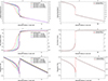 |
Fig. 1. Radial profiles of number density (top), radial speed (middle), and temperature (bottom) for a slow (left column) and a fast solar wind (right column) in the range from 1 R⊙ to 1 AU. These solutions were obtained using a heating function as given in Eq. (3). The color-coding distinguishes the discontinuous analytical solutions from the numerical ones. The slow wind solutions are computed for different widths of the heating function with corresponding different critical distances, where ϵ and ΔR = rc − r0 are given in units of solar radii. For the fast wind, a solution with an extremely narrow heating function is shown (ϵ = 1/64 R⊙, rc ≈ 6 R⊙). |
Evidently, solving the standard solar-wind equations with additional localized heating produces, however, quasi-discontinuous solutions that are close to the analytical solutions for a small width. As one can see at the example of the slow wind (left column), with decreasing width of the heating function the critical distances of the quasi-discontinuous (S) and the discontinuous solar-wind solution (A) become nearer to each other and the agreement improves. Within the limit of vanishing width, QH(r) becomes a delta function, with which the analytical solutions are formally obtained. This is illustrated with the plots for the fast wind solution (right column), where instead of the converging sequence of solutions, only one is shown for a very small width of the heating function: obviously, both solutions are in very good agreement.
Next, we confirmed that the quasi-discontinuous, fast solar-wind solution for ϵ = 0.5 R⊙ and rc = 6.8034 R⊙ in the steady-state model is truly stable by computing it with the time-asymptotic model. We chose this width as a representation of an acceptable spatial resolution of the heating function. The results can be seen in Fig. 2, where the analytical discontinuous solution (A) is indicated by the dotted black line, the steady-state model (S) by the solid red line, and the time-asymptotic model (T) by the 700 blue crosses between 1.3 R⊙ and 25.0 R⊙, which is the simulation range.
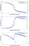 |
Fig. 2. Radial profiles of number density (top), radial speed (middle), and temperature (bottom) for a discontinuous and quasi-discontinuous fast solar wind solution in double logarithmic scaling to detect every deviation on all scales in the range from 1 R⊙ to 30 R⊙. The discontinuous solution (black dotted line) was analytically obtained by the procedure of Shergelashvili et al. (2020), the steady state solution (solid red line) was obtained numerically using a heating function as given in Eq. (3), and the time-asymptotic solution (blue crosses) was obtained numerically using the CRONOS code with the corresponding heating function as described with Eq. (9). The time-asymptotic solution gives the structure ten days after the switch to the quasi-discontinuous solar wind solution was set up. |
As is evident from Fig. 2, the time-asymptotic model (T) fits perfectly with the steady-state solution (S). The only deviation is in the upstream region, where the physical properties of the solar wind, which is derived time asymptotically, are weakly oscillating around the steady-state model. However, these deviations, which are due to the non-fixed (extrapolated) inner boundary condition for the flow velocity (see above), are very small. Obviously, the overall (time-averaged) structure is identical to the steady-state solution.
4. Sensitivity of the solutions to effects caused by a strong temperature gradient
In the previous section, we show that we can reconstruct the discontinuous analytic solutions as an idealized limit with a continuous solar-wind model explicitly containing a heating function. This way, we prove the validity and relevance of the new solutions introduced in an idealized setup analytically in Shergelashvili et al. (2020), which is the central result of the present study. While particular consequences of various possible and necessary refinements (see Sect. 5) will be subjects of forthcoming work, we briefly address potential impacts of the most obvious neglected processes that one could expect to change the solution due to a strong temperature gradient: namely heat conduction and the thermoelectric field.
4.1. Heat conduction
Depending on the heating function width ϵ, the resulting solutions have steep gradients in the physical quantities. This raises the question of how big the effect of heat conduction would be on these solutions and whether it would destroy their characteristic shapes. Therefore, we calculate the resulting heat conduction term Qcon(r) from the steady-state solutions, which would be included as an additional source term in Eq. (2). We limit the calculation of the heat conduction to electron-electron interaction, because other interactions are much smaller and, thus, negligible. To calculate the heat conduction term, we used the formulation for heat conductivity from Richardson (2019), which is based on Braginskii (1965) (see also Spitzer & Härm 1953). This formulation is in the cgs system of units, except the temperature, which is in eV; so, the Boltzmann constant formally becomes kB = 1.60 × 10⁻¹² erg eV−1. Then, the Coulomb logarithm can be written as
![Mathematical equation: $$ \begin{aligned} \lambda _{\rm e}=23.5-\ln \left(n_{\rm e}^\frac{1}{2}T^{-\frac{5}{4}}\right)-\left[10^{-5}+\frac{(\ln T-2)^2}{16}\right]^\frac{1}{2} ,\end{aligned} $$](/articles/aa/full_html/2024/06/aa47491-23/aa47491-23-eq12.gif) (11)
(11)
with the number density of electrons ne = 0.5n (i.e., approximated by half of the total number density). The collision time is then
 (12)
(12)
with me and e denoting electron mass and charge. The thermal conductivity κe = 3.2nekBTτe/me is needed to compute the electron heat flux:
 (13)
(13)
The heat conduction “source” term Qcon can then be formulated as
 (14)
(14)
and, subsequently, transformed into the SI system of units again.
The result for the slow wind with the heat function width ϵ = 1 R⊙ can be seen in the upper panel of Fig. 3. In principle, one can see two different regions where heat conductivity is noticeably present. These are the innermost region (below two solar radii), where heat is conducted outwards, and the region around the maximum temperature. There, the energy is dispersed in both directions, which could influence the shape of the resulting steady-state solution. Therefore, we need an indication as to when the heat conduction is not negligible. We chose to calculate a term we named ‘ratio of absolute powers’, ϕ, which is defined by
 (15)
(15)
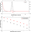 |
Fig. 3. Influence of heat conduction on quasi-discontinuous solar wind solutions. Upper panel shows heating function QH, T (black, Eq. (3)); heat conduction source term Qcon (red, Eq. (14)) for an exemplary slow solar wind solution (ϵ = 1 R⊙) is shown in the range from 1 R⊙ to 1 AU. Bottom panel shows ratio of absolute powers ϕ as a function of the heating function width ϵ for the slow (black) and fast (red) solar wind solutions. |
with Qρ = ρvr2 = const. being the mass flow constant. Here, rmin = r0 − 1.5ϵ and rmax = r0 + 8.0ϵ are defined in such a way that the whole dispersion region around the local temperature maximum is integrated, but not the region closer to the Sun. The resulting ratio for the example case given in the upper panel of Fig. 3 is ϕ = 0.11, which fits well with the visual impression of a rather weak influence of heat conduction on the source terms. For the following, we assume that as long as ϕ < 0.5, it is acceptable to neglect heat conduction in our solar-wind models.
In the bottom panel of Fig. 3, the ratio of absolute powers ϕ is shown in terms of the dependence of the heating function width ϵ both for the slow and fast solar-wind solutions. For the slow wind, widths greater than one third of a solar radius are acceptable. However, for the fast wind, only for widths above ϵ ≈ 2 R⊙ is the heat conduction small enough. The reason for this difference is that, overall, the temperature is higher in the fast solar wind; additionally, the temperature heating strength TH and the temperature gradient in this region are larger. So, particularly for the slow wind, the effect of the heat conduction becomes negligible despite rather steep temperature gradients (see Fig. 1).
We note that for a lower threshold value for ϕ, the minimum widths will of course increase, which may rule out the formation of such solutions in the fast solar wind. However, even when heat conduction is non-negligible but yet not dominant, it would lead to a further smoothing of the quasi-discontinuous solutions. While a heating function with a small width in combination with heat conduction would result in solar-wind solutions that do not have very steep (but still significant) gradients in the physical quantities, the overall structure of these solutions would be preserved even in such cases. Obviously, testing this quantitatively for a wider parameter range requires including the heat conduction self-consistently, which is, however, beyond the scope of the present paper; this work is mainly aimed at demonstrating that the idealized analytical solutions can be obtained as asymptotic cases of solutions derived for explicitly implemented heating functions.
4.2. Thermoelectric field
It has been argued in the literature (see, e.g., Landi & Pantellini 2001; Pantellini & Landi 2001) that conditions occur in the solar wind for which the thermoelectric field must be taken into account. This field, known from basic plasma physics (e.g., Golant et al. 1980; Hinton 1983), is the plasma physical analogon to the Seebeck effect in metals and obeys E = −α(kB/e)(dT/dr) with α ≈ 0.7. Simply including the effect of this field on the protons in the above-one-fluid-momentum equation allows us to give an upper limit of its influence. A comparison of the solution without and with this field at the example of the temperature profile of the slow wind with ϵ = 1/4 R⊙ (see lower left panel of Fig. 1) is displayed in Fig. 4 and demonstrates that, despite different temperatures, the principle character of the solution is unchanged.
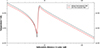 |
Fig. 4. Effect of thermoelectric field on temperature profile. Temperature profile of a steady-state slow solar wind solution based on a heating function is shown with a width of ϵ = 1/4 R⊙, with (solid red line) and without (black dotted line) thermoelectric field. |
5. Summary and conclusions
We present spherically symmetric, partially adiabatic solar-wind models explicitly containing a strongly localized heating source in order to asymptotically reproduce the analytically derived discontinuous solar-wind solutions introduced by Shergelashvili et al. (2020). We first demonstrated that the latter solutions can indeed be obtained in the limit of a vanishing width of the heating function from the solutions of a steady-state model. The fact that the steady-state solutions themselves can be obtained as time-asymptotic limits from those of a time-dependent model manifests the stability of the computed quasi-discontinuous solar wind profiles. Furthermore, it could be shown that heat conduction and the thermoelectric field are negligible up to a minimal heating function width. Therefore, the overall structure of the solutions persists, especially with the slow-wind solutions. Based on these findings, we expect to find the quasi-discontinuous solutions more likely in slow-wind regimes.
This first simplified model, which has the main objective of shedding more light on the previously derived analytical solutions, provides a good starting point to investigate various topics. An extension of the model to more spatial dimensions; to two fluids (protons and electrons), which allows a better treatment of the heat conduction; or including magnetic fields and time-dependent heating sources will be subjects of forthcoming analyses, as will be the formulation of non ad hoc heating functions that are derived from explicit dissipation processes for example local wave energy sources (see, e.g., Ismayilli et al. 2018; Shergelashvili et al. 2007, 2005 and references therein). The occurrence of such local spontaneous energy sources is naturally justified for the thermodynamically and statistically non-equilibrium solar atmosphere (Maes et al. 2009a,b). Subsequently, an application of the new solutions to recent solar-wind measurements taken with the Parker Solar Probe and Solar Orbiter may be helpful for their interpretation.
Acknowledgments
The work of L.W and B.S. was supported by Shota Rustaveli Georgian National Science Foundation grant for Fundamental Research – FR-23-10719. We thank the referees for constructive remarks that contributed to improve the presentation of the model significantly. We are also grateful for the help by Jens Kleimann with setting up the CRONOS code for application to the problem described. We acknowledge partial financial support for B.S. from the Ruhr-Universität Bochum (RUB) with in the VIP programme and from the Deutscher Akademischer Austauschdienst (DAAD) within EU fellowships for Georgian researchers, 2023 (57655523) – project Ref. ID. 91862684. We also thankfully acknowledge financial support for L.W. from the Cusanuswerk.
References
- Braginskii, S. I. 1965, Rev. Plasma Phys., 1, 205 [Google Scholar]
- Dormand, J., & Prince, P. 1980, J. Comp. Appl. Math., 6, 19 [CrossRef] [Google Scholar]
- Fichtner, H., Vormbrock, N., & Sreenivasan, S. 2000, AdSpR, 25, 1935 [NASA ADS] [Google Scholar]
- Fox, N. J., Velli, M. C., Bale, S. D., et al. 2016, Space. Sci. Rev., 204, 7 [NASA ADS] [CrossRef] [Google Scholar]
- Golant, V., Zhilinsky, A., & Sakharov, I. 1980, Fundamentals of Plasma Physics (New York: John Wiley& Sons) [Google Scholar]
- Hartle, R. E., & Barnes, A. 1970, J. Geophys. Res., 75, 6915 [NASA ADS] [CrossRef] [Google Scholar]
- Hartle, R. E., & Sturrock, P. A. 1968, ApJ, 151, 1155 [NASA ADS] [CrossRef] [Google Scholar]
- Hinton, F. L. 1983, in Handbook of Plasma Physics, 1, 147 [Google Scholar]
- Ismayilli, R. F., Dzhalilov, N. S., Shergelashvili, B. M., Poedts, S., & Pirguliyev, M. S. 2018, Phys. Plasmas, 25, 062903 [NASA ADS] [CrossRef] [Google Scholar]
- Keppens, R., & Goedbloed, J. P. 2000, ApJ, 530, 1036 [NASA ADS] [CrossRef] [Google Scholar]
- Kissmann, R., Kleimann, J., Krebl, B., & Wiengarten, T. 2018, ApJS, 236, 53 [Google Scholar]
- Kleimann, J. 2005, PhD Thesis, Ruhr University, Bochum, Germany [Google Scholar]
- Koehn, G. J., Desai, R. T., Davies, E. E., et al. 2022, ApJ, 941, 139 [NASA ADS] [CrossRef] [Google Scholar]
- Laitinen, T., Fichtner, H., & Vainio, R. 2003, J. Geophys. Res., 108, 1081 [NASA ADS] [Google Scholar]
- Lamers, H. J. G. L. M., & Cassinelli, J. P. 1999, Introduction to Stellar Winds (Cambridge: Cambridge University Press) [Google Scholar]
- Landi, S., & Pantellini, F. G. E. 2001, A&A, 372, 686 [NASA ADS] [CrossRef] [EDP Sciences] [Google Scholar]
- Lawrence, F. S. 1986, Math. Comput., 46, 135 [CrossRef] [Google Scholar]
- Maes, C., Netocny, K., & Shergelashvili, B. 2009a, Lecture Notes in Mathematics (Berlin: Springer Verlag), 1970, 247 [Google Scholar]
- Maes, C., Netočný, K., & Shergelashvili, B. M. 2009b, Phys. Rev. E, 80, 011121 [NASA ADS] [CrossRef] [Google Scholar]
- Manchester, W. B., Gombosi, T. I., Roussev, I., et al. 2004, J. Geophys. Res. (Space Phys.), 109, A01102 [NASA ADS] [Google Scholar]
- McCrea, W. H. 1956, ApJ, 124, 461 [CrossRef] [Google Scholar]
- Melnik, V. N., Brazhenko, A. I., Konovalenko, A. A., et al. 2014, Sol. Phys., 289, 263 [CrossRef] [Google Scholar]
- Müller, D., Marsden, R. G., St Cyr, O. C., & Gilbert, H. R., 2013, Sol. Phys., 285, 25 [CrossRef] [Google Scholar]
- Pantellini, F., & Landi, S. 2001, Ap&SS, 277, 149 [NASA ADS] [CrossRef] [Google Scholar]
- Parker, E. N. 1958, ApJ, 128, 664 [Google Scholar]
- Parker, E. N. 1965, Space. Sci. Rev., 4, 666 [NASA ADS] [CrossRef] [Google Scholar]
- Priest, E. R. 1982, Solar Magneto-hydrodynamics., 21 [CrossRef] [Google Scholar]
- Richardson, A. 2019, 2019 NRL Plasma Formulary (Naval Research Laboratory) [Google Scholar]
- Shergelashvili, B. M., & Fichtner, H. 2012, ApJ, 752, 142 [NASA ADS] [CrossRef] [Google Scholar]
- Shergelashvili, B. M., Zaqarashvili, T. V., Poedts, S., & Roberts, B. 2005, A&A, 429, 767 [NASA ADS] [CrossRef] [EDP Sciences] [Google Scholar]
- Shergelashvili, B. M., Maes, C., Poedts, S., & Zaqarashvili, T. V. 2007, Phys. Rev. E, 76, 046404 [NASA ADS] [CrossRef] [Google Scholar]
- Shergelashvili, B. M., Melnik, V. N., Dididze, G., et al. 2020, MNRAS, 496, 1023 [NASA ADS] [CrossRef] [Google Scholar]
- Spitzer, L., & Härm, R. 1953, Phys. Rev., 89, 977 [Google Scholar]
- Steinolfson, R. S., Suess, S. T., & Wu, S. T. 1982, ApJ, 255, 730 [NASA ADS] [CrossRef] [Google Scholar]
- Tsinganos, K. 1996, AdSpR, 17, 65 [NASA ADS] [Google Scholar]
- Tu, C.-Y., & Marsch, E. 1995, Space. Sci. Rev., 73, 1 [NASA ADS] [CrossRef] [Google Scholar]
- Usmanov, A. V., Matthaeus, W. H., Goldstein, M. L., & Chhiber, R. 2018, ApJ, 865, 25 [Google Scholar]
All Figures
|
Fig. 1. Radial profiles of number density (top), radial speed (middle), and temperature (bottom) for a slow (left column) and a fast solar wind (right column) in the range from 1 R⊙ to 1 AU. These solutions were obtained using a heating function as given in Eq. (3). The color-coding distinguishes the discontinuous analytical solutions from the numerical ones. The slow wind solutions are computed for different widths of the heating function with corresponding different critical distances, where ϵ and ΔR = rc − r0 are given in units of solar radii. For the fast wind, a solution with an extremely narrow heating function is shown (ϵ = 1/64 R⊙, rc ≈ 6 R⊙). |
| In the text | |
|
Fig. 2. Radial profiles of number density (top), radial speed (middle), and temperature (bottom) for a discontinuous and quasi-discontinuous fast solar wind solution in double logarithmic scaling to detect every deviation on all scales in the range from 1 R⊙ to 30 R⊙. The discontinuous solution (black dotted line) was analytically obtained by the procedure of Shergelashvili et al. (2020), the steady state solution (solid red line) was obtained numerically using a heating function as given in Eq. (3), and the time-asymptotic solution (blue crosses) was obtained numerically using the CRONOS code with the corresponding heating function as described with Eq. (9). The time-asymptotic solution gives the structure ten days after the switch to the quasi-discontinuous solar wind solution was set up. |
| In the text | |
|
Fig. 3. Influence of heat conduction on quasi-discontinuous solar wind solutions. Upper panel shows heating function QH, T (black, Eq. (3)); heat conduction source term Qcon (red, Eq. (14)) for an exemplary slow solar wind solution (ϵ = 1 R⊙) is shown in the range from 1 R⊙ to 1 AU. Bottom panel shows ratio of absolute powers ϕ as a function of the heating function width ϵ for the slow (black) and fast (red) solar wind solutions. |
| In the text | |
|
Fig. 4. Effect of thermoelectric field on temperature profile. Temperature profile of a steady-state slow solar wind solution based on a heating function is shown with a width of ϵ = 1/4 R⊙, with (solid red line) and without (black dotted line) thermoelectric field. |
| In the text | |
Current usage metrics show cumulative count of Article Views (full-text article views including HTML views, PDF and ePub downloads, according to the available data) and Abstracts Views on Vision4Press platform.
Data correspond to usage on the plateform after 2015. The current usage metrics is available 48-96 hours after online publication and is updated daily on week days.
Initial download of the metrics may take a while.