| Issue |
A&A
Volume 685, May 2024
|
|
|---|---|---|
| Article Number | A59 | |
| Number of page(s) | 15 | |
| Section | Catalogs and data | |
| DOI | https://doi.org/10.1051/0004-6361/202245762 | |
| Published online | 06 May 2024 | |
Improving metallicity estimates for very metal-poor stars in the Gaia DR3 GSP-Spec catalog★
1
Kapteyn Astronomical Institute, University of Groningen,
Landleven 12,
9747 AD
Groningen, The Netherlands
e-mail: This email address is being protected from spambots. You need JavaScript enabled to view it.
2
Astronomisches Rechen-Institut, Zentrum für Astronomie der Universität Heidelberg,
Mönchhofstraße 12–14,
69120
Heidelberg, Germany
Received:
22
December
2022
Accepted:
31
January
2024
Abstract
Context. In the latest Gaia Data Release (DR3), the GSP-Spec module has provided stellar parameters and chemical abundances measured from the RVS spectra alone. However, the GSP-Spec parameters – including metallicity – for very metal-poor (VMP; [Fe/H] < −2) stars suffer from parameter degeneracy due to a lack of information in their spectra, and are therefore affected by a large measurement uncertainty and systematic offset. Furthermore, the recommended quality cuts filter out the majority (~80%) of the VMP stars because some of them are confused with hot stars or with cool K- and M-type giants, for which the current pipeline is known to have problems.
Aims. We aim to provide more precise metallicity estimates for VMP stars analyzed by the GSP-Spec module by taking photometric information into account in the analysis and breaking the degeneracy.
Methods. We reanalyzed FGK-type stars in the GSP-Spec catalog by computing the Ca triplet equivalent widths from the published set of GSP-Spec stellar parameters. We compared these recovered equivalent widths with the values directly measured from public Gaia RVS spectra and investigated the precision of the recovered values and the parameter range within which the recovered values are reliable. We then converted the recovered equivalent widths to metallicities by adopting photometric temperatures and surface gravities that we derive based on Gaia and 2MASS catalogs.
Results. The recovered equivalent widths agree with the directly measured values with a scatter of 0.05 dex for the stars that pass the GSP-Spec quality cuts. Among the stars recommended for filtering out, we observe a similar scatter for FGK-type stars initially misidentified as hot stars. Contrarily, we find a poorer agreement, in general, for stars that the GSP-Spec identifies as cool K- and M-type giants, although we can still define subsets that show reasonable agreement. At the low-metallicity end ([Fe/H] < −1.5), our metallicity estimates have a typical uncertainty of 0.18 dex, which is about half of the quoted GSP-Spec metallicity uncertainty at the same metallicity. Our metallicities also show better agreement with the high-resolution literature values than the original GSP-Spec metallicities at low metallicity; the scatter in the comparison decreases from 0.36–0.46 dex to 0.17−0.29 dex for stars that satisfy the GSP-Spec quality cuts. While the GSP-Spec metallicities show increasing scatter when misidentified “hot” stars and the subsets of the “cool K- and M-type giants” are included (up to 1.06 dex), we can now identify them as FGK-type stars and provide metallicities that show a small scatter in the comparisons (up to 0.34 dex), which helps us to increase the number of VMP stars with reliable and precise metallicity.
Conclusions. The inclusion of photometric information greatly contributes to breaking parameter degeneracy, enabling precise metallicity estimates for VMP stars from Gaia RVS spectra. We produce a publicly available catalog of bright metal-poor stars suitable for high-resolution follow-up. The sample contains about 2345 VMP stars with an estimated contamination rate of 5%.
Key words: methods: data analysis / catalogs / stars: abundances / stars: Population II
The catalog is available at the CDS via anonymous ftp to cdsarc.cds.unistra.fr (130.79.128.5) or via https://cdsarc.cds.unistra.fr/viz-bin/cat/J/A+A/685/A59
© The Authors 2024
 Open Access article, published by EDP Sciences, under the terms of the Creative Commons Attribution License (https://creativecommons.org/licenses/by/4.0), which permits unrestricted use, distribution, and reproduction in any medium, provided the original work is properly cited.
This article is published in open access under the Subscribe to Open model. This email address is being protected from spambots. You need JavaScript enabled to view it. to support open access publication.
1 Introduction
Low-metallicity stars provide us with unique opportunities to study astrophysical processes (Beers & Christlieb 2005; Frebel & Norris 2015), such as the formation and supernova explosion of the first stars (e.g., Ishigaki et al. 2018), nucleosynthesis of heavy elements by neutron-capture processes (e.g., Sneden et al. 2008), and the early assembly of the Milky Way (e.g., Chiba & Beers 2000; Yuan et al. 2020; Sestito et al. 2021). Therefore, extensive efforts have been devoted to searching for such stars from photometric observations (Schlaufman & Casey 2014; Starkenburg et al. 2017; Da Costa et al. 2019) and spectroscopy (Beers et al. 1985, 1992; Christlieb et al. 2008; Caffau et al. 2013; Aoki et al. 2013; Roederer et al. 2014; Aguado et al. 2016; Li et al. 2018; Matijevič et al. 2017). As very metal-poor stars (VMP; [Fe/H] < −2) are relatively rare among field stars, it is necessary both to observe a large number of stars and to develop an efficient method to select VMP stars among them.
The Gaia mission has provided fresh opportunities in this regard (Gaia Collaboration 2016). The recent Gaia Data Release 3 (Gaia Collaboration 2023b) is the first to provide stellar parameters and chemical abundances estimated from the spectra taken with the Radial Velocity Spectrometer (RVS; Cropper et al. 2018) instrument. The spectra cover the Ca triplet region (846–870 nm) with a resolution of R ~ 11 500, and are analyzed through the General Stellar Parametriser-spectroscopy, GSP-Spec module (Recio-Blanco et al. 2023). The current GSP-Spec catalog contains 5.6 million stars analyzed and is already one of the largest catalogs of stellar parameters derived from spectra; moreover, the number is expected to increase in future releases. By filtering out stars with suspicious solutions, Gaia Collaboration (2023a) demonstrate that the estimated astrophysical quantities are of excellent quality.
Although the wavelength coverage of the RVS spectra is known to be suitable for searching for VMP stars (e.g., Starkenburg et al. 2010; Matijevič et al. 2017), there is a limitation in the current GSP-Spec parameters for this purpose. The main difficulty is the small number of lines detected in the spectra of VMP stars (Kordopatis et al. 2011; Recio-Blanco et al. 2016). In the fully spectroscopic approach, which is adopted in the current version of the GSP-Spec module, at least three parameters must be determined simultaneously, namely effective temperature (Teff), surface gravity (log g), and metallicity ([M/H])1. Although this is possible for stars of solar metallicity, it gets more challenging for VMP stars, whose spectra lack spectral signatures needed for parameter determination (Recio-Blanco et al. 2023). Therefore, a number of filtering methods need to be applied when studying metal-poor stars in the GSP-Spec catalog, and the precision in [M/H] is not as good as for solar-metallicity stars even after the filtering.
The difficulty is illustrated in Fig. 1, where we compare GSP-Spec metallicity with Li et al. (2022) for 109 stars. As the metallicity estimates by Li et al. (2022) are based on highresolution spectroscopy and homogeneous analysis, we can consider them reliable and precise. Figure 1 shows that the GSP-spec module struggles to provide accurate metallicities at very low metallicity. Not only do the GSP-Spec metallicities have large uncertainties, which likely reflects strong parameter degeneracy, but there is also a large population of stars for which GSP-Spec systematically overestimates metallicity and underestimates its uncertainty (see the third quadrant of the bottom panel). The agreement is improved by filtering out stars with a set of quality cuts used by Recio-Blanco et al. (2023) for studying the metallicity distribution function, which we refer to as MP-filtering throughout this paper. However, only 23 out of 109 stars (21%) survive this filtering. We present a more detailed discussion on this comparison and the limitation of GSP-Spec in Sect. 2.
However, the bottom panel of Fig. 1 shows that it is possible to improve the metallicity agreement for stars removed by the MP filter. There is a clear sequence between metallicity and temperature discrepancies among many of the VMP stars, indicating that most of the poor solutions are due to the degeneracy between [Fe/H] and Teff. If we were able to shift Teff closer to the high-resolution Teff, we would expect the metallicity to also be shifted closer to the high-resolution value. In this work, we incorporate photometric and astrometric information of stars into the analysis in order to provide more precise and accurate metallicity for VMP stars. As spectra are publicly available for only 18% of the stars analyzed by the GSP-Spec module, we are not able to reanalyze spectra directly. Instead, we assume that we can infer the observed spectra using the published GSP-Spec stellar parameters and remeasure metallicities from them. We describe this method in detail in Sect. 3. Using public RVS spectra and highresolution surveys, we then validate the assumption, investigate the range where the assumption holds, and provide uncertainties to our new metallicities in Sect. 4. In Sect. 5, we present properties of VMP and extremely metal-poor (EMP; [Fe/H] < −3) stars selected based on our new metallicity, and discuss possible caveats and future prospects. We present a summary in Sect. 6.
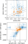 |
Fig. 1 Comparisons of stellar parameters between GSP-Spec and a high-resolution spectroscopic study of VMP stars by Li et al. (2022). (Top) Comparison of the metallicities from optical high-resolution spectroscopy with the GSP-Spec metallicity for VMP stars from Li et al. (2022). (Bottom) Relation between Teff and [Fe/H] discrepancies. The orange points show stars that satisfy the filters introduced by Recio-Blanco et al. (2023) for constructing the metallicity distribution function. |
2 VMP stars in the GSP-Spec catalog
Here, we discuss the properties of VMP stars in the GSP-Spec catalog using the sample of Li et al. (2022). These VMP stars are originally selected from the low-resolution survey (R ~ 1800) of Large Sky Area Multi-Object Fibre Spectroscopic Telescope (LAMOST; Cui et al. 2012; Zhao et al. 2012) using the method described by Li et al. (2018) for the high-resolution follow-up observations with the Subaru telescope as described by Aoki et al. (2022). As the sample includes rather faint stars, GSP-Spec parameters are available for only 109 out of the total of 385 stars. While the median uncertainty in the metallicity estimates by Li et al. (2022) is 0.11 dex, that in the GSP-Spec metallicities is 0.79 dex. Due to this large uncertainty in the GSP-Spec, the two metallicities are consistent within 1 sigma for more than half of the stars. However, a significant fraction (18%) of the stars show a discrepancy more significant than the 2 sigma level. Therefore, while the GSP-Spec uncertainty describes the majority of the discrepancy, there is a significant fraction of stars for which the measurement uncertainty is underestimated. The GSP-Spec metallicity tends to be higher than the high-resolution value, indicating that the stars hit the GSP-Spec grid edge.
One might consider that the metallicity agreement in Fig. 1 depends on the signal-to-noise ratio of the RVS spectra.
Figure 2 shows the metallicity difference as a function of S/N, with each point color-coded according to the Teff from Li et al. (2022). The figure demonstrates that good agreement is achieved only when the star satisfies the MP filters, is relatively cool (Teff(Li + 22) ≲ 5500 K), and has a high S/N of ≳50. This is likely a reflection of the weak spectral feature of very metal-poor stars; in the parameter range of VMP stars, it is common to see an increased number of spectral features in the higher-S/N spectra of cooler stars.
One might also argue that VMP stars could tend to have low S/N given that they are rare and in the halo, which would affect the quality of parameter estimates. The sample of 109 VMP stars has a median RVS S/N of 36.6, and 25 and 75 percentiles are 26.9 and 47.4. These numbers can be compared to the 25–50–75 percentiles for all the stars in the entire GSP-Spec, which are 26.8, 37.3, and 60.3. Therefore, while the median S/N of VMP stars is not different from the entire sample, there is a significant lack of high-S/N spectra. The overall significant mismatch seen in Fig. 1 is likely due to the combined effect of the low fraction of high-S/N spectra among the 109 VMP stars as well as the high S/N required for precise parameter determination of VMP stars.
It is clear in Fig. 2 that having high S/N and cool temperature alone is not sufficient for VMP stars to have a precise metallicity from the GSP-Spec catalog. The set of MP filters needs to be applied in order to select stars with precise metallicity estimates from the GSP-Spec. The filtering process removes stars with potential parameter bias due to large broadening velocity and large uncertainty on the radial velocity, stars whose parameter solution is outside of the training grid, hot stars with Teff > 6000 K, those classified as O- or B-type stars by the Extended Stellar Parameteriser of Hot Stars (ESP-HS), cool giants (K and M-type giants), and stars with high gravity (log g > 4.9); more details can be found in Recio-Blanco et al. (2023).
As discussed in Sect. 1, the filtering process removes about 80% of VMP stars. In this study, we also aim to keep more VMP stars – even after quality cuts – by dropping or relaxing some of the criteria used in the MP filter, in particular Tgspspec ≤ 6000 (and log ≤ 4.9) and KMgiantPar, which are responsible for removing many VMP stars (see Table 1). These two criteria were introduced to remove very hot OBA-type stars, which can be affected by the grid border at Teff = 8000 K, and cool giants with initial Teff estimates of < 4000 K, which can suffer parameterization issues due to the pseudo-continuum caused by molecular absorptions. VMP stars in Li et al. (2022) removed by these two criteria would have been significantly affected by the parameter degeneracy; true VMP stars should not be classified as cool giants when there is no degeneracy, because they typically have 4200 K ≲ Teff. As they can be up to Teff ~ 6700 K, those removed by Tgspspec ≤ 6000 K might not be misclassified due to the parameter degeneracy. However, hot stars are more likely to suffer from parameter degeneracy because of the lack of features in their spectra. While GSP-Spec and Li et al. (2022) do not agree on the metallicity of stars removed by the two criteria, we expect that photometric and astrometric information helps us to break the degeneracy, separate metal-poor stars from cool giants and hot OBA-type stars, and obtain precise metallicity, allowing us to increase the sample size of metal-poor stars with reliable and precise metallicity.
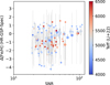 |
Fig. 2 Metallicity difference between Li et al. (2022) and GSP-Spec as a function of S/N. Bigger points are for stars that pass MP-filters, and all the points are color-coded according to the Teff adopted by Li et al. (2022). |
The number of VMP stars removed by each condition.
3 Method
3.1 Photometric Teff and log g
Here, we provide independent Teff and log g for stars in the current GSP-Spec catalog using photometry and astrometry. As these stellar parameters do not rely on RVS spectra, we expect them to help us break the degeneracy among parameters.
We use Gaia and the Two Micron All Sky Survey (2MASS Skrutskie et al. 2006) as sources of photometric information. We first cross match stars analyzed by the GSP-Spec module with the Gaia main source catalog and the 2MASS point source catalog (Cutri et al. 2003) using the 2MASS best neighbor catalog in Gaia DR3 (gaiadr3.tmass_psc_xsc_best_neighbour). We primarily use three-dimensional extinction maps by Green et al. (2019) and Marshall et al. (2006) to deredden the photometries. For stars that are not covered by either of the three-dimensional maps, we scale the two-dimensional map by Schlegel et al. (1998), assuming a sech2 profile for dust distribution, where the scale height was assumed to be 125 pc (Marshall et al. 2006). The extinction laws are taken from the values presented in Casagrande et al. (2021) for Cardelli et al. (1989) and O’Donnell (1994) extinction laws.
We estimate the photometric Teff using G – Ks color when 2MASS Ks-band magnitude has a quality “A” or “B”; otherwise, we use Gaia BP – RP color. We adopt color-temperature relations by Mucciarelli et al. (2021), around which there are dispersions of about 50–60 K. We adopt the nearest edge value of the range for stars with metallicity values outside the calibration range. We discard stars falling outside the color range in which the relations are calibrated.
We then compute the log g of stars from their luminosities (L). Combined with the photogeometric distance by Bailer-Jones et al. (2021), we obtain L from Ks-band if it was measured with the aforementioned quality, or from G-band otherwise, using the bolometric correction of Casagrande & VandenBerg (2014, 2018)2. We then derive the log g of stars from  , where the stellar mass M is assumed to be 0.7 M⊙ for stars with log g > 3.5 and 0.8 M⊙ for log g < 3.5. Although the assumption of mass can be inaccurate for some stars, it does not affect our conclusions, because we are interested in metal-poor stars, which are known to be old. In addition, the effect of M is minimized when converting the gravity to the log scale for constructing model atmospheres.
We estimate the typical uncertainty of log g as follows. If a star has 20% distance fractional uncertainty, it contributes 0.17 dex to the log g uncertainty. However, as the measured distances of GSP-Spec stars tend to be precise, with a median fractional distance uncertainty of 1.9%, the typical contribution from the distance is only 0.016 dex. The Teff does not contribute to the log g uncertainty either; 60 K uncertainty in Teff translates to 0.017 uncertainty in log g. The dominant source of log g uncertainty is the assumed mass. Low-metallicity stars usually have a mass of within 0.1 M⊙ from the assumed mass, which would translate to 0.05–0.07 dex log g uncertainty. The effect of mass can be larger for high-metallicity stars, which can be young. For example, if a star has 1.6 M⊙ instead of 0.8 M⊙ assumed in the analysis, we would underestimate log g by 0.3 dex.
3.2 Remeasuring metallicity
The RVS spectra are usually dominated by the Ca triplet feature. We therefore assume that the GSP-Spec solution provides a reasonable fit to the Ca triplet even when the solution suffers from degeneracy. This assumption is justified by the distribution of  , which quantifies the residual between the best-fit spectrum and the observed spectrum. The median log
  are −3.06 and −2.93 for the stars in common between the MP sample and Li et al. (2022) and for the remaining stars from Li et al. (2022), respectively, indicating that the goodness of the fits does not significantly depend on whether the star satisfies the MP filters3. We can also visually confirm the assumption in Fig. 3, which compares published RVS spectra with synthetic spectra for two stars selected from Li et al. (2022). One of the stars passes the MP filters and has a precise metallicity from the GSP-Spec (0.30 dex), while the other does not pass the filters and has a large uncertainty (0.95, dex). We calculated the two synthetic spectra for the published GSP-Spec parameters and the high-resolution parameters and abundances in a way that is consistent with the GSP-Spec module; we use Turbospectrum v19.1 (Plez 2012) with MARCS model atmospheres (Gustafsson et al. 2008) and the same line data for the Ca triplet as that presented in Contursi et al. (2021). For the microturbulence, we assume the relation in Buder et al. (2021) for the GALAH survey, as that used by the GSP-Spec module is not publicly available. The good match among the three spectra – regardless of how well the GSP-Spec parameters agree with high-resolution values or whether or not a star passes the MP filters – is encouraging. We further validate the assumption in Sect. 4.1.
Based on this assumption, we first compute Ca triplet equivalent widths from the published values of stellar parameters and then rederive the Ca abundances of stars using the Teff and log g from the previous section using the software, model atmospheres, line data, and microturbulence described above. For computational reasons, we adopt interpolation in a pre-constructed grid for the analysis. The grid provides equivalent widths for the three Ca lines as a function of Teff, log g, and [Ca/H]. We only use models with standard chemical compositions, which have the following relation between [α/M] and [M/H]:
![Mathematical equation: $[\alpha /{\rm{Fe}}] = \left\{ {\matrix{ {0.4} \hfill & {\left( {\left[ {{{{\rm{Fe}}} \mathord{\left/ {\vphantom {{{\rm{Fe}}} {\rm{H}}}} \right. \kern-\nulldelimiterspace} {\rm{H}}}} \right]\, \le \, - 1.0} \right)} \hfill \cr { - 0.4\left[ {{{{\rm{Fe}}} \mathord{\left/ {\vphantom {{{\rm{Fe}}} {\rm{H}}}} \right. \kern-\nulldelimiterspace} {\rm{H}}}} \right]} \hfill & {\left( { - 1.0\, > \,\left[ {{{{\rm{Fe}}} \mathord{\left/ {\vphantom {{{\rm{Fe}}} {\rm{H}}}} \right. \kern-\nulldelimiterspace} {\rm{H}}}} \right]\, > \,0.0} \right).} \hfill \cr {0.0} \hfill & {\left( {0 \le \left[ {{{{\rm{Fe}}} \mathord{\left/ {\vphantom {{{\rm{Fe}}} {\rm{H}}}} \right. \kern-\nulldelimiterspace} {\rm{H}}}} \right]} \right)} \hfill \cr } } \right.$](/articles/aa/full_html/2024/05/aa45762-22/aa45762-22-eq4.png) (1)
(1)
The [Ca/H] in our grid is equal to [α/Η].
As the first step, we estimate the equivalent widths of the Ca triplet using the GSP-Spec stellar parameters: Teff, log g, [M/H], and [α/M]. We convert the reported [M/H] and [α/M] to [α/H] and take this value as the input [Ca/H]. As we aim to mitigate the difficulty in the global fitting of spectra, we use the global stellar parameters rather than using abundances of individual elements such as [Ca/Fe]. In this process, GSP-Spec only varies the four parameters, not individual abundances. When a star does not have a reported [α/M], we use Eq. (1) to convert [M/H] to [Ca/H]. For stars with Teff > 4000 and log g > 5.0, we adopt log g = 5.0, as these are not represented in our model grid.
Using the adopted Teff and log g from the previous section, we measure Ca abundance from each of the three lines from the estimated equivalent widths. We take the median of the three estimates for the adopted value of [Ca/H]. We finally convert the Ca abundance to metallicity assuming Eq. (1). As both the photometric temperature and bolometric correction require a predetermined metallicity, we start with the GSP-Spec metallicity and iterate the whole process three times to ensure convergence.
4 Validation
In this section, we validate our assumption that we can recover the Ca triplet equivalent widths from the GSP-Spec parameters and compare our new metallicities with previous studies. Through these validations, we introduce new quality cuts and estimate the typical uncertainty in our new metallicity.
4.1 The recovery of equivalent widths
We investigate how well we can recover the equivalent widths of the Ca triplet based on the assumption in Sect. 3.2 by comparing the recovered values with the values directly measured from spectra. We use public RVS spectra, which are available for ~18% of the stars in the GSP-Spec catalog. As we are mostly interested in low-metallicity stars, we downloaded all the public RVS spectra for 1934 stars, which have [Fe/H] < −2 in our new metallicity. We then fitted a Voigt profile to each of the three Ca triplet lines to measure equivalent widths.
Figure 4 compares the recovered and directly measured equivalent widths. Here, we define 〈Δ logEW〉 as log(EWrecovered/EWdirect) averaged over the three lines. The good agreement between the two equivalent widths is clear among the MP sample; the 16, 50, and 84 percentiles in 〈ΔlogEW〉 are −0.01, 0.02, and 0.08 (Table 2).
However, the dispersion is significantly larger than the fitting uncertainty in EWdirect, which is typically σ(log EW) < 0.01 dex. Therefore, the dominant source of the dispersion should be due to what is not accounted for in the uncertainty estimates in EWdirect- A possible source of dispersion is the error due to our assumption that we can recover the equivalent widths from the published GSP-Spec parameters. In particular, we do not account for the uncertainties in the GSP-Spec parameters. However, we find that taking into account the uncertainties on the GSP-Spec parameters is not straightforward because we do not have access to the full Monte Carlo sampling of GSP-Spec parameters or the covariance among the parameters, which is crucial when estimated parameters suffer from significant degeneracy. From error propagation, we have the following relation between the uncertainty on the recovered equivalent widths and those on stellar parameters:
 (2)
(2)
where ξi is a stellar parameter, and  is the covariance between two stellar parameters. As we do not have access to
  , we have to assume them to be zero. Under this assumption, the median σ(EWrecovered) is ~0.15–0.16 dex for the MP sample, which is significantly larger than the dispersion in Fig. 4 (0.03–0.06 dex). This overestimation would likely be due to the significant correlation between parameters; for example, while
  and
and ![Mathematical equation: ${\rm{ }}{{\partial {\rm{EW}}} \over {\partial {{[{\rm{Fe}}/{\rm{H}}]}_{{\rm{gspspec }}}}}}$](/articles/aa/full_html/2024/05/aa45762-22/aa45762-22-eq9.png) are negative and positive, respectively,
are negative and positive, respectively, ![Mathematical equation: ${\rho _{{T_{{\rm{eff,gspspec }}}},{{[{\rm{Fe}}/{\rm{H}}]}_{{\rm{gspspec }}}}}} = {\sigma _{{T_{{\rm{eff,gspspec }}}},{{[{\rm{Fe}}/{\rm{H}}]}_{{\rm{gspspec}}}}}}/{\sigma _{{T_{{\rm{eff,gspspec }}}}}}{\sigma _{{{[{\rm{Fe}}/{\rm{H}}]}_{{\rm{gspspec}}}}}}$](/articles/aa/full_html/2024/05/aa45762-22/aa45762-22-eq10.png) seems positive and significantly larger than zero (see Fig. 1). Therefore, the term including
seems positive and significantly larger than zero (see Fig. 1). Therefore, the term including ![Mathematical equation: $\sigma {T_{{\rm{eff,gspspec }}}},{[{\rm{Fe}}/{\rm{H}}]_{{\rm{gspspec}}}}$](/articles/aa/full_html/2024/05/aa45762-22/aa45762-22-eq11.png) reduces the estimated uncertainty. As we are not able to take this term into account, we should naturally expect that we are likely to overestimate σ (EWrecovered).
reduces the estimated uncertainty. As we are not able to take this term into account, we should naturally expect that we are likely to overestimate σ (EWrecovered).
We therefore conclude that it is not possible to estimate σ (EWrecovered) from the currently available information. We therefore adopt an empirical approach to estimate the error caused by our assumption in Sect. 3.2. For the MP sample, we estimate σ (log EW) to be 0.05 from the dispersion in the comparison presented in Fig. 4.
Figure 4 also shows that the Ca triplet equivalent widths are recovered for some of the stars that do not satisfy the MP filters. Motivated by this, here we try to relax some of the quality cuts adopted by Recio-Blanco et al. (2023), especially those effective in filtering out true VMP stars (Table 1).
Figure 5 presents 〈Δ log EW〉 across the GSP-Spec Kiel diagram for stars that do not survive the MP filters. We divide the stars into five boxes, labeled A–E, depending on their positions in the diagram. The figure clearly shows that our method successfully recovers the equivalent widths for stars in regions A and B, even though they do not satisfy the MP filters. Stars in region A of Fig. 5 survive all the cuts on stellar parameters in the MP filter but are removed by the other cuts; more specifically, vbroad[TGM]>1 and vrad[TGM]>1. The good recovery for the stars in region B shows that it is possible to retain more warm metal-poor stars, which are originally removed by requiring Teff,gspspec < 6000 K in the MP filters (see Table 1). For stars in regions A and B, the (16, 50, and 84) percentiles of 〈Δ log EW〉 are (−0.02, 0.05, 0.10) and (−0.02, 0.05, 0.10), respectively (Table 2). These values are similar to what we found for the MP sample. On the other hand, our method fails to recover the Ca triplet equivalent widths for the majority of the stars in regions C and D.
Here, we discuss region E separately. The region E corresponds to Teff,gspspec = 4250 K and log ggspspec = 1.5, and all the stars in this region have KMgiantPar > 0. Any improvement for this subsample is critical in retaining a larger number of metal-poor stars (see Table 1). While the recovery of equivalent widths for these stars seems challenging in general, an additional space, defined by [Fe/H]gspspec − log ![Mathematical equation: ${[{\rm{Fe}}/{\rm{H}}]_{{\rm{gspspec}}}} - \log \chi _{{\rm{gspspec}}}^2$](/articles/aa/full_html/2024/05/aa45762-22/aa45762-22-eq13.png) , provides the possibility to rescue some stars in this category by making a further cut. Figure 6 shows that the fraction of stars showing good agreement between direct measurements and recovered values changes as a function of log
, provides the possibility to rescue some stars in this category by making a further cut. Figure 6 shows that the fraction of stars showing good agreement between direct measurements and recovered values changes as a function of log  and [Fe/H]gspspec. In particular, the agreement seems reasonably good for two regions, namely that (E1) definedas [Fe/H]gspspec > −3 and log
  < −2.0 and another (E2) defined as [Fe/H]gspspec = 3.51. For stars in regions E1 and E2, the (16, 50, and 84) percentiles of 〈Δ logEW〉 are (−0.01, 0.10, 0.26) and (0.12, 0.20, 0.30), respectively (Table 2).
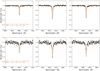 |
Fig. 3 Comparison of observed RVS spectra (shown as black dots) with synthetic spectra (orange solid and gray dashed lines). The orange and gray spectra are reproduced with GSP-Spec and Li et al. (2022) parameters, respectively. The latter study is based on high-resolution spectroscopy (HR). The top and bottom panels are for a star that satisfies the MP filters with 0.30 dex metallicity uncertainty (Gaia DR3 927340858625174656) and for one that does not, with a large uncertainty of 0.95 dex (Gaia DR3 2682719929806900096). The parameters assumed in the syntheses are shown in the panels in the following order: Teff, log g, [Fe/H], and [α/Fe] ([Ca/Fe] in case of HR. Our approach is to infer a new metallicity based on the orange spectrum, as not every star in the GSP-Spec catalog has a publicly available observed spectrum. |
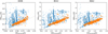 |
Fig. 4 Comparisons of the equivalent widths recovered based on the assumption in Sect. 3.2 with those directly measured from spectra. Symbols follow Fig. 1. |
Equivalent width comparisons.
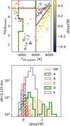 |
Fig. 5 The 〈Δ log EW〉 values across the Kiel diagram for stars that are filtered out by the MP filters. We define five regions labeled A–E in the Kiel digram and investigate stars in each region. The boundary of region A is defined by the cuts made in MP filters (Recio-Blanco et al. 2023, see Table 1). |
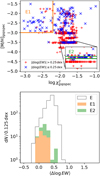 |
Fig. 6 The 〈Δ log EW〉 for stars with KMgiantPar > 0. The top panel shows the distribution of stars that show good agreement between recovered and directly measured equivalent widths (red) and those that show poor agreement (blue). Here, we define two regions E1 and E2 in [Fe/H]gspspec – log |

4.2 Relaxing filters, uncertainties, and outliers
Based on the validation presented in the previous subsection, here we define four types of quality cuts and present a typical uncertainty in our newly derived metallicity for each sample. Before relaxing the quality cuts, here we introduce additional quality cuts to remove stars for which our method is expected to perform poorly. As we rely on photometry and astrometry, the precision of stellar parameters degrades for stars with high extinction or poor distance estimation. Our method also performs less well with hot stars and cool dwarfs because our assumption that the Ca triplet dominates the RVS spectra does not hold for these objects. While hydrogen lines start contaminating the Ca triplet in hot stars, the Ca triplet strengths are no longer sensitive to the metallicity in cool dwarfs (see Fig. 7). To mitigate all these effects, we introduce additional filters on extinction (E(B – V) < 0.72), distance precision (2dphotogeo,med/(dphotogeo,hi – dphotgeo,lo) > 3), and on our photometric stellar parameters (Teff < 7000 K, and Teff > 5000 K or log g < 3.0).
The first sample combines these additional quality cuts and the MP filters, and we call it the MP+ sample. Some of the conditions are then dropped or relaxed to form the RMP sample following the investigation of the previous section. Specifically, we drop the conditions on vbroad[TGM] and vrad[TGM], and relax the condition on stellar parameters to include stars in region B of Fig. 4. We further extend the sample by including stars in sample E1 of the previous section, which has KMgiantPar = 1, [M/H]gspspec > −3, and log  < −2.2 (eRMP1 sample), and then those in E2, which have KMgiantPar = 1 and [Fe/H]gspspec = −3.51 (eRMP2 sample). These sets of quality cuts and samples are summarized in Appendix A.
For the stars in the MP+ and RMP samples, we adopt σ(log EW) = 0.05 dex as the uncertainty in the recovered equivalent widths (Table 2). We note that we ignored the small offset between EWrecovered and EWdirect because the offset may simply be due to the mismatch between observed and synthetic spectra at the cores of the Ca triplet. As we use the same approach when recovering equivalent widths and remeasuring metallicities, we consider that the effect of the offset will be canceled out. We apply corrections to the recovered equivalent widths for stars newly added in the eRMP1 and eRMP2 samples, as the offsets found for these samples are different from what we found for the MP sample. We shift the recovered equivalent widths by −0.05 and −0.15 dex in log(EW) for these stars, respectively, based on the difference in the median 〈Δ log EW〉 values between the MP and eRMP samples (Table 2). Similarly, we adopt 0.13 and 0.14 dex uncertainties for them.
Taking into account the typical uncertainties in our stellar parameters, Teff (60 K) and log g (0.08 dex), and those in the recovered equivalent widths, we estimate the uncertainty in remeasured metallicity for individual objects. The typical metallicity uncertainties (the number of objects) are 0.32 (3134736), 0.30 (4 109 821), 0.30 (4 142 936), and 0.30 (4 143 310) dex for MP+, RMP, eRMP1, and eRMP2 samples. In all cases, the contribution of σ (log EW) is by far the largest; even for the MP+ sample, σ (log EW) makes contributions that are approximately five and ten times those of σ(Teff) and σ(log g), respectively. However, we note that these uncertainties are estimated using stars with [Fe/H] < −2 in our new metallicity estimates. As we show in the following section, higher metallicity stars seem to have smaller uncertainties.
Here, we discuss the fraction of significant failures for each sample, that is, where our metallicities are significantly incorrect. We define the significant failures as those showing > 0.2 dex difference between the recovered and directly measured equivalent widths. This 0.2 dex equivalent width difference can move a star with [Fe/H]= −2 to ~ – 1.4. The fractions of the catastrophic failures are small for the MP+ and RMP samples (2% and 1.5 %, respectively). Stars in eRMP1 or eRMP2, but not in RMP, have higher fractions of 14–20%, making the total fractions of the failures 4% and 5% for the entire eRMP1 and eRMP2 samples.
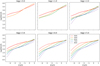 |
Fig. 7 Curve of growth for the Ca line at 8498 Å. Colors show different Teff. Dashed lines are used for Teff,phot > 7000 K, and Teff,phot < 5000 K and log gphot > 3.0 as they are not included in the final sample given that the Ca lines can be contaminated by hydrogen lines in relatively hot stars and their strengths are not sensitive to the Ca abundance in cool dwarfs (see the two right panels in the bottom row). Similar figures for the other two lines are available in Appendix B. |
4.3 Metallicity comparison with the literature
In this section, we validate the results via metallicity comparisons with the spectroscopic surveys APOGEE DR17 and GALAH DR3, and the high-resolution study by Li et al. (2022). We remove stars with STAR_BAD or FE_H_FLAG flagged from the APOGEE sample and those with flag_sp ≠ 0 or flag_fe_h ≠ 0 from the GALAH sample. We use the Li et al. (2022) sample to study our precision at the very metal-poor regime. We note that we applied the calibration given in Table 3 of Recio-Blanco et al. (2023) for the GSP-Spec metallicities in the comparisons.
The comparisons of the upper panels (GSP-Spec results) and lower panels (our result) of Fig. 8 show that our method significantly reduces the dispersion at low metallicity and removes outliers. The lower panels show a bimodal sequence at high metallicity ([Fe/H] ≳ −0.5), which can be explained by the α-rich and α-poor disk populations, and our assumption of the single relation between [α/Fe] and [Fe/H]. The GSP-Spec module provides [α/Fe] measurements with a typical precision of 0.04 dex. The measured [α/Fe] values show a dispersion of 0.11 dex around our assumed [α/Fe] ratio from Eq. (1), which might be considered as an additional source of error. Nonetheless, our method still provides reasonable metallicities even for such high-metallicity stars.
One significant improvement is the reduction in the number of cases where the metallicity estimates are significantly far from the high-resolution value at low metallicity. Here, we investigate the fraction of stars with a metallicity offset of larger than 0.5 dex compared to high-resolution studies without making any quality cuts. In the published GSP-Spec catalog, the fractions are 76% in the sample of Li et al. (2022), and 49% and 43% among the stars with [Fe/H]HR < −1.5 in APOGEE and GALAH. With our newly derived metallicities, these fractions drop to 24, 29, and 19% , respectively.
While the improvement at low metallicity is clear, there are stars for which our metallicities still show significant disagreement when compared to high-resolution values, indicating that we need to filter out some stars. We adopt the quality cuts described in the previous section to ensure that our updated stellar parameters do not suffer from reddening, poor photometry, or poor astrometry, that the Ca triplet features of stars are sensitive to metallicity and are the dominant feature in RVS spectra, and that we can recover the Ca triplet equivalent widths from the published GSP-Spec parameters.
We first discuss MP+ filters, which are a combination of the quality cuts introduced by Recio-Blanco et al. (2023) and those on photometric stellar parameters. It is clear in Fig. 8 that the MP+ filters mostly remove stars that show a poor agreement in metallicity. While both the original GSP-Spec metallicity and our new metallicity show good agreement with high-resolution studies within this MP+ sample, there is still a noticeable improvement in our metallicity compared to the GSP-Spec value: we have fewer false VMP stars than the GSP-Spec analysis. Even with the MP+ filtering, there is a clump of stars at [M/H]gspspec ~ −2 and [Fe/H]HR ~ −0.5 in the top panels of APOGEE and GALAH comparisons, which are false VMP stars. This clump disappears in the corresponding lower panels as they move closer to the one-to-one relation.
Provided with the result of the previous section, here we replace the MP filters with more relaxed sets of conditions. We remove or relax some of the filters step by step and validate each step in Fig. 9. The first two rows of Fig. 9 correspond to the RMP filters, and the third and last rows correspond to the eRMP1 and eRMP2 filters, respectively. The figure demonstrates that the agreements remain great for the RMP sample, and reasonably good for eRMP samples.
We quantify these agreements with APOGEE, GALAH, and VMP stars from Li et al. (2022) for the samples in Table 3. It is clear that while our new metallicity agrees with APOGEE and GALAH to as good a degree as the GSP-Spec original metallicity for the entire MP+ sample, the agreement is significantly improved at low metallicity. At [Fe/H] < −1.5, our metallicity has much smaller offsets (−0.01–0.02 dex compared to 0.15−0.14 dex) and smaller dispersions (0.17–0.19 dex compared to 0.36–0.38 dex). In the comparison with Li et al. (2022)4, our metallicity has a larger offset (0.21 dex compared to 0.19 dex) and a smaller dispersion (0.29 dex compared to 0.43 dex). This might indicate that there is a metallicity-dependent offset because of systematic uncertainties in the analysis (see Sect. 5.2), since the sample of Li et al. (2022) is more biased toward low metallicity than the two surveys. Alternatively, it is also possible that the metallicity scale of Li et al. (2022) has an offset from APOGEE and GALAH surveys.
Our estimate of uncertainties seems reasonable for low-metallicity stars. At [Fe/H] < −1.5, our new metallicity has a typical uncertainty of 0.18 dex, which is about 55% of the typical GSP-Spec metallicity uncertainty and close to the dispersions found in the comparisons with APOGEE and GALAH. Although this is smaller than the dispersion in the comparison with Li et al. (2022), this sample of VMP stars has the largest uncertainty among the literature measurements we use (0.11 dex). Therefore, we consider that our estimates of uncertainties are reasonable and that our method provides more precise metallicities for low-metallicity stars than the GSP-Spec module.
On the other hand, the typical metallicity uncertainty is much larger when using our method (0.32 dex) than that achieved with GSP-Spec (0.06 dex) for the entire sample. This indicates that the GSP-Spec module performs excellently for high-metallicity stars because there is enough information in their RVS spectra and it already utilizes spectral features to constrain stellar parameters. Despite the larger uncertainty in our method, the dispersions in comparisons remain small, indicating that our uncertainty is likely overestimated at high metallicity. This over-estimation is not unexpected given that we used stars with [Fe/ H] < −2 to estimate uncertainties in the recovered equivalent widths and the recovered equivalent widths might have higher accuracy at higher metallicity. As the GSP-Spec already provides stellar parameters with high quality for high-metallicity stars, one can adopt GSP-Spec metallicities for such stars, and therefore we do not try to provide more realistic uncertainties for high-metallicity stars. The similar dispersions in the two comparisons are expected also because our method does not return a significantly different metallicity if GSP-Spec stellar parameters already agree with photometric estimates; this would likely be the case for high-metallicity stars that do not have degeneracy issues.
Table 3 also contains comparisons with RMP and eRMP samples. It is clear that the GSP-Spec original metallicities show a large scatter at [Fe/H] < −1.5 when we use the RMP and eRMP samples, while our new metallicity estimates in the three samples are as good as in the MP+ sample. We also note that the numbers of VMP stars from Li et al. (2022) in RMP and eRMP samples increase significantly compared to the MP sample (from 22 to 64 and 76 stars used for the comparisons, respectively). This demonstrates the power of photometric information for the analysis of the spectra of low-metallicity stars.
We finally comment on stars that have high metallicity in our estimates ([Fe/H] > −0.5) but low metallicity in GALAH ([Fe/H] < −1.5). Most of these stars are either around (α, δ) = (155.63°, −44.31°) with the GALAH field_id 4205 or around (225.93°, −77.02°) with the field_id 2620. As they have the value ‘2’ in the 11th digit of sobject_id, they might have been affected by the stacking issue in the GALAH DR3 (Buder et al. 2021).
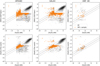 |
Fig. 8 Comparisons of [Fe/H] from surveys with that from our new metallicity estimates. For each plane, all stars with [Fe/H] < −1.5 in either axis of the panel are shown as individual data points. In all panels, gray points show all the stars available for the comparison, while the orange stars are for the MP+ sample, which combines the filters from Recio-Blanco et al. (2023) and our additional quality cuts in photometry, astrometry, and our photometric stellar parameters (see text for details). The solid and dashed lines show the one-to-one relation and the ±0.5 dex offset, respectively. Median uncertainties are presented in the top-left corner of each panel. |
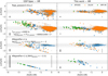 |
Fig. 9 Metallicity comparisons for stars that are added by our new relaxed filters. The text in the figure describes stars newly added in each step. For example, stars in the top panels satisfy all the conditions in the MP-filters except for flags_gspspec[0-6] ≤ 1. We refer the readers to Sect. 4.2 for more details. We use larger symbol sizes for stars that have [Fe/H] < −1.5 in one of the two metallicities being compared. The gray lines show Δ[Fe/H] = 0 and ±0.5 dex. We show median metallicity uncertainties for GSP-Spec and our measurements as vertical lines for stars with [Fe/H] < −1.5 on the left and for all the stars on the right. |
5 Discussion
5.1 Properties of our VMP stars
In this section, we summarize the properties of our VMP stars in RMP and eRMP2 samples and compare them with those of VMP stars in the MP sample. We focus on the metallicity and magnitude distributions and how the catalog of VMP stars changes by moving from the GSP-Spec analysis to our analysis.
Figure 10 shows the metallicity distribution functions for our RMP and eRMP2 samples created with our new metallicity estimates, which are also compared with the original [M/H]gspspec distribution from the MP sample. The number of VMP stars and extremely metal-poor (EMP) stars (with [Fe/H] < −3) remain approximately the same, and the overall shape of the metallicity distribution is unchanged. We find 1790 VMP and 85 EMP stars with calibrated [M/H]gspspec and the MP-filters, 1989 VMP and 40 EMP stars in our new metallicities with RMP filters, and 2417 VMP and 44 EMP stars with eRMP filters. Although the number of VMP stars remains similar, only 826 in the first sample of VMP stars remain in the RMP VMP sample. As noted in Sect. 4.3, this is partly thanks to the removal of false VMP stars when moving from the GSP-Spec metallicity to our measurements. The remaining approximately 1000 stars are now not regarded as VMP stars in our new metallicity estimates. The reduction in the number of VMP stars is then compensated by our relaxed filters described in Sect. 4.2.
The relaxed filters are particularly efficient in keeping known low-metallicity stars. In addition to the significant increase in the overlap with the Li et al. (2022) sample mentioned above, we can also confirm the effect of the relaxed filters by looking at how many VMP and EMP stars in RMP and eRMP2 samples are in the MP sample. Of the 1989 VMP and 40 EMP stars in the RMP sample, only 71% and 23% are in the MP sample. The corresponding values for the eRMP sample are 60% and 21%. About 30–40% of VMP stars and ~80% of EMP stars could not have been identified if we had not tried to relax the MP filters.
Our RMP sample offers one of the best and brightest metal-poor star catalogs to date. As they have been analyzed by the GSP-Spec module, most stars are brighter than G = 13 (Fig. 10). Such bright stars are easily followed up with high-resolution spectroscopy for detailed abundance measurements. One can also use the eRMP samples, but they have larger uncertainties.
Metallicity comparisons with high-resolution studies.
5.2 Caveat and future prospects
Although we have significantly improved the accuracy of the metallicity for very metal-poor stars, there are limitations in this approach. First, the spectra are unavailable for ~80% of the stars, making it impossible to start directly from spectra or visually check the fitting results. While statistically there is good agreement between high-resolution metallicities and our new ones, there could be very rare cases where the spectrum and/or the stellar parameters have issues; for example because of flux contamination from nearby bright stars, the presence of unresolved companions, and/or stellar activity and rotation. Visually checking the fitting result is useful, especially when one wants to remove such rare cases for follow-up observations of high-confidence EMP stars. The fraction of these stars is to be estimated from such follow-up observations.
Second, while the use of photometric information greatly contributes to breaking the degeneracy, it introduces a dependency on photometric measurements and extinction estimates. One of the advantages of fully spectroscopic analysis is that all the spectra can be analyzed consistently without the analysis being affected by the coverage of photometric surveys and dust maps. While our approach negates this advantage of the GSP-Spec module, we consider that the gain more than compensates for this issue for very metal-poor stars.
While we use additional photometric information to that provided by Gaia, it should, in principle, be possible to obtain photometric stellar parameters from the Gaia BP/RP spectra. We refrain from using the GSP-Phot analysis results of the Gaia BP/RP spectra as they currently suffer from systematic offsets (Andrae et al. 2023). Thus, future improvements to the GSP-Phot module would also benefit the analysis of the RVS spectra of VMP stars.
Here, we provide new metallicities based on the local thermodynamic equilibrium (LTE) assumption. As non-LTE effects are known to be significant for the Ca triplet (Mashonkina et al. 2007; Sitnova et al. 2019; Osorio et al. 2022), our metallicities are subject to deviation from the LTE assumption. Here, we focus on the LTE analysis because grids of the correction do not span the whole parameter space we explore, and we aim to maintain the consistency with the GSP-Spec analysis as much as possible, which adopts the LTE assumption. As the abundance obtained from LTE analyses of the Ca triplet is generally higher than that obtained from non-LTE analyses, our metallicities are likely overestimated. The metallicity dependence of this effect may be related to the median offset we find only in comparison with Li et al. (2022) in Table 3.
One challenge we have is how to include more stars with KMgiantPar flagged. Many VMP stars are mistaken with higher metallicity cool giants with significant molecule features. The spectra of these latter stars mimic the spectra of VMP stars with weak and shallow absorption lines due to a pseudo continuum. A better understanding of how we can separate these types of stars would significantly benefit the search for VMP and EMP stars from the RVS spectra.
As we no longer need to break the degeneracy between stellar parameters, the use of photometric information may allow us to derive metallicities from RVS spectra with a lower signal-to-noise ratio than the current threshold. As seen in the sample size of stars with radial velocity measurements in Gaia DR2 (down to G ~ 13, 7.2 million stars Gaia Collaboration 2018) and Gaia DR3 (down to G ~ 14, 33 million stars Gaia Collaboration 2023b), we expect a significant increase in the sample size by going deeper.
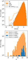 |
Fig. 10 Metallicity and magnitude distributions of stars. (Top) Orange histograms show the metallicity distribution functions in our new metallicities with different sets of filters. The gray line indicates the MDF from the GSP-Spec [M/H]. (Bottom) Magnitude distribution of our VMP and EMP stars in RMP and eRMP filters. |
6 Summary
While the GSP-Spec module provides precise spectroscopic stellar parameters and chemical abundances for most of the sample, the analysis suffers from parameter degeneracy at the very low metallicity regime. As a result, many of the known very metal-poor stars have large metallicity uncertainties and fail to pass quality cuts. We mitigate this difficulty by incorporating photometric information into the analysis; we provide improved metallicities with smaller uncertainty for low-metallicity stars, and aim to keep more very metal-poor stars even after some quality cuts. We first computed the Ca triplet equivalent widths from the published set of GSP-Spec parameters using Turbospectrum. We then converted the equivalent widths back to metallicity assuming photo-astrometric Teff and log g. Our new Ca triplet metallicity shows a better agreement with the high-resolution value for the sample of very metal-poor stars by Li et al. (2022).
Our main findings can be summarized as follows:
We conducted an independent validation of the GSP-Spec metallicities using the high-resolution spectroscopic study of very metal-poor stars by Li et al. (2022). For a sample satisfying the recommended set of filters by Recio-Blanco et al. (2023), the GSP-Spec metallicity shows reasonable agreement with Li et al. (2022). However, this set of filters (MP filters) leaves only 23 stars out of 109 with high-resolution and GSP-Spec metallicities. Moreover, even the 23 stars have large uncertainty (median uncertainty of 0.44 dex). Despite even larger uncertainties (0.82 dex), stars that do not satisfy this quality cut show disagreements in metallicity and temperature beyond the measurement uncertainties, which would likely be due to parameter degeneracy (Fig. 1).
Even if a star suffers from parameter degeneracy, we can reproduce the strengths of the Ca triplet reasonably well with the published GSP-Spec parameters (Fig. 3 and Sect. 4.1). We confirmed this by directly measuring the Ca triplet equivalent widths from public Gaia RVS spectra and comparing them with our reproduced values. We further investigated how the precision of the recovered equivalent widths changes in GSP-Spec stellar parameter space and defined subsamples for which we can reasonably recover the equivalent widths (Sect. 4.2). These subsamples include stars that Recio-Blanco et al. (2023) recommend should be filtered out, such as stars with Teff,GSP-Spec > 6000 K and cool K and M-type giant stars.
This motivates us to re-derive metallicities from the recovered Ca triplet equivalent widths by adopting a new set of Teff and log g derived from photometry and astrometry.
The new Ca triplet metallicity shows good agreement with high-resolution values at low metallicity and reasonable agreement even at high metallicity (Fig. 8). The new metal-licity has a typical uncertainty of 0.18 dex at [Fe/H] < −1.5, which is 45% smaller than the median GSP-Spec uncertainty at the same metallicity. This method also reduces the fraction of catastrophic failure at low metallicity, where the metallicity estimates are different from high-resolution values by more than 0.5 dex. This fraction is now 24% with our new metallicity, while it is 76% in the original GSP-Spec metallicity.
We are now able to consider our metallicity as reliable for 64 stars out of the aforementioned 109 very metal-poor stars. This number goes up to 76 if we adopt our most extended sample. For the sample of 64 and 76 stars, the mean differences (± standard deviation) compared to the Li et al. (2022) values are 0.22 (±0.25) and 0.24 (±0.34) dex, respectively.
Our sample offers one of the best catalogs of very bright low-metallicity stars. The numbers of VMP and EMP stars are 1989 and 40 stars. In the most extended sample, these numbers increase to 2417 and 44, but this comes with a low level of metal-rich contaminants. We estimate the fraction of significant failures to be low (≲ 5%) even for the most extended sample from the equivalent widths comparison; however, this fraction needs to be further constrained with future follow-up observations. We make the catalog available online.
As discussed in Sect. 5.2, while the use of photometric information confers certain advantages, especially for stars with little information in their spectra due to low metallicity or low signal-to-noise ratio, it introduces a dependency on external data sets. For example, the present work relies on 2MASS and extinction maps from multiple studies. Future data releases from Gaia with improved GSP-Photo stellar parameters might enable us to conduct a similar analysis to the present study: a spectroscopic analysis with photometric information using only Gaia data.
Acknowledgements
We thank the referee for her constructive comments based on her extensive knowledge and experience in the field, which significantly improved the quality of the paper. We thank Georges Kordopatis at Université Côte d’Azur for his helpful comments. This research has been supported by a Spinoza Grant from the Dutch Research Council (NWO). ES acknowledges funding through VIDI grant “Pushing Galactic Archaeology to its limits” (with project number VI.Vidi.193.093) which is funded by the Dutch Research Council (NWO). We benefited from support from the International Space Science Institute (ISSI) in Bern, CH, thanks to the funding of the Team “the early Milky Way”. This work has made use of data from the European Space Agency (ESA) mission Gaia (https://www.cosmos.esa.int/gaia), processed by the Gaia Data Processing and Analysis Consortium (DPAC, https://www.cosmos.esa.int/web/gaia/dpac/consortium). Funding for the DPAC has been provided by national institutions, in particular the institutions participating in the Gaia Multilateral Agreement.
Appendix A Summary of our quality cuts
In the main text, we define the following samples.
MP+ sample, which is combination of the filters by Recio-Blanco et al. (2023) and filtering on photometric parameters:
3500 ≤ Teff,gspspec ≤ 6000
log ggspspec ≤ 4.9
Teff,gspspec ≥ 4150 or log ggspspec ≤ 2.4 or log ggspspec ≥ 3.8
vbroad[TGM]=0 and vrad[TGM]=0
extrapol ≤ 2
K MgiantPar = 0
spectraltype_esphs is not O or B
2dphotogeo,med/(dphotogeo,hi – dphotgeo,lo) > 3
E(B – V) < 0.72
Teff,photo < 7000
Teff,photo > 5000 or log gphoto < 3.0.
RMP sample, which relaxes or removes some of the conditions in the MP+ filtering:
3500 ≤ Teff,gspspec
Teff,gspspec ≤ 6000 or log ggspspec ≥ (Teff,gspspec − 6000)/1000 + 3
Teff,gspspec ≥ 6000 or log ggspspec ≤ 4.9
Teff,gspspec ≥ 4150 or log ggspspec ≤ 2.4 or log ggspspec ≥ 3.8
extrapol ≤ 2
KMgiantPar = 0
spectraltype_esphs is not O or B
2dphotogeo,med/(dphotogeo,hi – dphotgeo,lo) > 3
E(B – V) < 0.72
Teff,photo < 7000
Teff,photo > 5000 or log gphoto < 3.0.
eRMP1 sample, which extends the RMP sample by including some stars with KMgiantPar flagged:
3500 ≤ Teff,gspspec
Teff,gspspec ≤ 6000 or log ggspspec ≥ (Teff,gspspec – 6000)/1000 + 3
Teff,gspspec ≥ 6000 or log ggspspec ≤ 4.9
Teff,gspspec ≥ 4150 or log ggspspec ≤ 2.4 or log ggspspec ≥ 3.8
extrapol ≤ 2
KMgiantPar = 0 or (KMgiantPar = 1 and log
 and [M/H]gspspec > −3)
spectraltype_esphsis not O or B
2dphotogeo,med/(dphotogeo,hi – dphotgeo,lo) > 3
E(B – V) < 0.72
Teff,photo < 7000
Teff,photo > 5000 or log gphoto < 3.0.
eRMP2 sample, which further extends the eRMP1 sample by including more stars with KMgiantPar flagged:
3500 ≤ Teff,gspspec
Teff,gspspec ≤ 6000 or log ggspspec ≥ (Teff,gspspec – 6000)/1000 + 3
Teff,gspspec ≥ 6000 or log ggspspec ≤ 4.9
Teff,gspspec ≥ 4150 or log ggspspec ≤ 2.4 or log ggspspec ≥ 3.8
extrapol ≤ 2
KMgiantPar = 0 or (KMgiantPar = 1 and log
 and [M/H]gspspec > −3) or (KMgiantPar = 1 and [M/H]gspspec = −3.51)
spectraltype_esphs is not O or B
2dphotogeo,med/(dphotogeo,hi – dphotgeo,lo) > 3
E(B – V) < 0.72
Teff,photo < 7000
Teff,photo > 5000 or log gphoto < 3.0.
Appendix B Curve of growth for Ca 8552 and 8662 lines
References
- Aguado, D. S., Allende Prieto, C., González Hernández, J. I., et al. 2016, A&A, 593, A10 [NASA ADS] [CrossRef] [EDP Sciences] [Google Scholar]
- Andrae, R., Fouesneau, M., Sordo, R., et al. 2023, A&A, 674, A27 [CrossRef] [EDP Sciences] [Google Scholar]
- Aoki, W., Li, H., Matsuno, T., et al. 2022, ApJ, 931, 146 [NASA ADS] [CrossRef] [Google Scholar]
- Aoki, W., Beers, T. C., Lee, Y. S., et al. 2013, AJ, 145, 13 [CrossRef] [Google Scholar]
- Bailer-Jones, C. A. L., Rybizki, J., Fouesneau, M., Demleitner, M., & Andrae, R. 2021, AJ, 161, 147 [Google Scholar]
- Beers, T. C., & Christlieb, N. 2005, ARA&A, 43, 531 [NASA ADS] [CrossRef] [Google Scholar]
- Beers, T. C., Preston, G. W., & Shectman, S. A. 1985, AJ, 90, 2089 [NASA ADS] [CrossRef] [Google Scholar]
- Beers, T. C., Preston, G. W., & Shectman, S. A. 1992, AJ, 103, 1987 [NASA ADS] [CrossRef] [Google Scholar]
- Buder, S., Sharma, S., Kos, J., et al. 2021, MNRAS, 506, 150 [NASA ADS] [CrossRef] [Google Scholar]
- Caffau, E., Bonifacio, P., Sbordone, L., et al. 2013, A&A, 560, A71 [NASA ADS] [CrossRef] [EDP Sciences] [Google Scholar]
- Cardelli, J. A., Clayton, G. C., & Mathis, J. S. 1989, ApJ, 345, 245 [Google Scholar]
- Casagrande, L., & VandenBerg, D. A. 2014, MNRAS, 444, 392 [Google Scholar]
- Casagrande, L., & VandenBerg, D. A. 2018, MNRAS, 479, L102 [NASA ADS] [CrossRef] [Google Scholar]
- Casagrande, L., Lin, J., Rains, A. D., et al. 2021, MNRAS, 507, 2684 [NASA ADS] [CrossRef] [Google Scholar]
- Chiba, M., & Beers, T. C. 2000, AJ, 119, 2843 [NASA ADS] [CrossRef] [Google Scholar]
- Christlieb, N., Schörck, T., Frebel, A., et al. 2008, A&A, 484, 721 [NASA ADS] [CrossRef] [EDP Sciences] [Google Scholar]
- Contursi, G., de Laverny, P., Recio-Blanco, A., & Palicio, P. A. 2021, A&A, 654, A130 [NASA ADS] [CrossRef] [EDP Sciences] [Google Scholar]
- Cropper, M., Katz, D., Sartoretti, P., et al. 2018, A&A, 616, A5 [NASA ADS] [CrossRef] [EDP Sciences] [Google Scholar]
- Cui, X.-Q., Zhao, Y.-H., Chu, Y.-Q., et al. 2012, Res. Astron. Astrophys., 12, 1197 [Google Scholar]
- Cutri, R. M., Skrutskie, M. F., van Dyk, S., et al. 2003, 2MASS All Sky Catalog of point sources [Google Scholar]
- Da Costa, G. S., Bessell, M. S., Mackey, A. D., et al. 2019, MNRAS, 489, 5900 [NASA ADS] [CrossRef] [Google Scholar]
- Frebel, A., & Norris, J. E. 2015, ARA&A, 53, 631 [NASA ADS] [CrossRef] [Google Scholar]
- Gaia Collaboration (Prusti, T., et al.) 2016, A&A, 595, A1 [NASA ADS] [CrossRef] [EDP Sciences] [Google Scholar]
- Gaia Collaboration (Brown, A. G. A., et al.) 2018, A&A, 616, A1 [NASA ADS] [CrossRef] [EDP Sciences] [Google Scholar]
- Gaia Collaboration (Recio-Blanco, A., et al.) 2023a, A&A, 674, A38 [CrossRef] [EDP Sciences] [Google Scholar]
- Gaia Collaboration (Vallenari, A., et al.) 2023b, A&A, 674, A1 [NASA ADS] [CrossRef] [EDP Sciences] [Google Scholar]
- Green, G. M., Schlafly, E., Zucker, C., Speagle, J. S., & Finkbeiner, D. 2019, ApJ, 887, 93 [NASA ADS] [CrossRef] [Google Scholar]
- Gustafsson, B., Edvardsson, B., Eriksson, K., et al. 2008, A&A, 486, 951 [NASA ADS] [CrossRef] [EDP Sciences] [Google Scholar]
- Ishigaki, M. N., Tominaga, N., Kobayashi, C., & Nomoto, K. 2018, ApJ, 857, 46 [Google Scholar]
- Kordopatis, G., Recio-Blanco, A., de Laverny, P., et al. 2011, A&A, 535, A106 [NASA ADS] [CrossRef] [EDP Sciences] [Google Scholar]
- Li, H., Tan, K., & Zhao, G. 2018, ApJS, 238, 16 [CrossRef] [Google Scholar]
- Li, H., Aoki, W., Matsuno, T., et al. 2022, ApJ, 931, 147 [NASA ADS] [CrossRef] [Google Scholar]
- Marshall, D. J., Robin, A. C., Reylé, C., Schultheis, M., & Picaud, S. 2006, A&A, 453, 635 [NASA ADS] [CrossRef] [EDP Sciences] [Google Scholar]
- Mashonkina, L., Korn, A. J., & Przybilla, N. 2007, A&A, 461, 261 [NASA ADS] [CrossRef] [EDP Sciences] [Google Scholar]
- Matijevic, G., Chiappini, C., Grebel, E. K., et al. 2017, A&A, 603, A19 [NASA ADS] [CrossRef] [EDP Sciences] [Google Scholar]
- Mucciarelli, A., Bellazzini, M., & Massari, D. 2021, A&A, 653, A90 [NASA ADS] [CrossRef] [EDP Sciences] [Google Scholar]
- O’Donnell, J. E. 1994, ApJ, 422, 158 [Google Scholar]
- Osorio, Y., Aguado, D. S., Prieto, C. A., Hubeny, I., & González Hernández, J. I. 2022, ApJ, 928, 173 [NASA ADS] [CrossRef] [Google Scholar]
- Plez, B. 2012, Astrophysics Source Code Library [record ascl:1205.004] [Google Scholar]
- Recio-Blanco, A., de Laverny, P., Allende Prieto, C., et al. 2016, A&A, 585, A93 [NASA ADS] [CrossRef] [EDP Sciences] [Google Scholar]
- Recio-Blanco, A., de Laverny, P., Palicio, P. A., et al. 2023, A&A, 674, A29 [NASA ADS] [CrossRef] [EDP Sciences] [Google Scholar]
- Roederer, I. U., Preston, G. W., Thompson, I. B., et al. 2014, AJ, 147, 136 [Google Scholar]
- Schlaufman, K. C., & Casey, A. R. 2014, ApJ, 797, 13 [CrossRef] [Google Scholar]
- Schlegel, D. J., Finkbeiner, D. P., & Davis, M. 1998, ApJ, 500, 525 [Google Scholar]
- Sestito, F., Buck, T., Starkenburg, E., et al. 2021, MNRAS, 500, 3750 [Google Scholar]
- Sitnova, T. M., Mashonkina, L. I., Ezzeddine, R., & Frebel, A. 2019, MNRAS, 485, 3527 [NASA ADS] [CrossRef] [Google Scholar]
- Skrutskie, M. F., Cutri, R. M., Stiening, R., et al. 2006, AJ, 131, 1163 [NASA ADS] [CrossRef] [Google Scholar]
- Sneden, C., Cowan, J. J., & Gallino, R. 2008, ARA&A, 46, 241 [Google Scholar]
- Starkenburg, E., Hill, V., Tolstoy, E., et al. 2010, A&A, 513, A34 [CrossRef] [EDP Sciences] [Google Scholar]
- Starkenburg, E., Martin, N., Youakim, K., et al. 2017, MNRAS, 471, 2587 [NASA ADS] [CrossRef] [Google Scholar]
- Yuan, Z., Myeong, G. C., Beers, T. C., et al. 2020, ApJ, 891, 39 [NASA ADS] [CrossRef] [Google Scholar]
- Zhao, G., Zhao, Y.-H., Chu, Y.-Q., Jing, Y.-P., & Deng, L.-C. 2012, Res. Astron. Astrophys., 12, 723 [NASA ADS] [CrossRef] [Google Scholar]
The GSP-Spec module additionally varies [α/Fe] in this step.
We use an updated version available at https://github.com/casaluca/bolometric-corrections. We also use our reimplementation of their Python script for more efficient computation.
We remove stars with Teff,spspec = 4250 K and log ggspspec = 1.5 in this comparison as the MP filters have a cut in KMgiantPar, which depends on log  for stars that have these stellar parameters in the published catalog (Recio-Blanco et al. 2023). Such a cut can introduce a bias in the
We note that we remove Gaia DR3 4580919415339537280 from the comparison. This star is a hot Teff ~ 5800 K horizontal branch star and is the outlier in the bottom right panel of Fig. 8.
All Tables
All Figures
|
Fig. 1 Comparisons of stellar parameters between GSP-Spec and a high-resolution spectroscopic study of VMP stars by Li et al. (2022). (Top) Comparison of the metallicities from optical high-resolution spectroscopy with the GSP-Spec metallicity for VMP stars from Li et al. (2022). (Bottom) Relation between Teff and [Fe/H] discrepancies. The orange points show stars that satisfy the filters introduced by Recio-Blanco et al. (2023) for constructing the metallicity distribution function. |
| In the text | |
|
Fig. 2 Metallicity difference between Li et al. (2022) and GSP-Spec as a function of S/N. Bigger points are for stars that pass MP-filters, and all the points are color-coded according to the Teff adopted by Li et al. (2022). |
| In the text | |
|
Fig. 3 Comparison of observed RVS spectra (shown as black dots) with synthetic spectra (orange solid and gray dashed lines). The orange and gray spectra are reproduced with GSP-Spec and Li et al. (2022) parameters, respectively. The latter study is based on high-resolution spectroscopy (HR). The top and bottom panels are for a star that satisfies the MP filters with 0.30 dex metallicity uncertainty (Gaia DR3 927340858625174656) and for one that does not, with a large uncertainty of 0.95 dex (Gaia DR3 2682719929806900096). The parameters assumed in the syntheses are shown in the panels in the following order: Teff, log g, [Fe/H], and [α/Fe] ([Ca/Fe] in case of HR. Our approach is to infer a new metallicity based on the orange spectrum, as not every star in the GSP-Spec catalog has a publicly available observed spectrum. |
| In the text | |
|
Fig. 4 Comparisons of the equivalent widths recovered based on the assumption in Sect. 3.2 with those directly measured from spectra. Symbols follow Fig. 1. |
| In the text | |
|
Fig. 5 The 〈Δ log EW〉 values across the Kiel diagram for stars that are filtered out by the MP filters. We define five regions labeled A–E in the Kiel digram and investigate stars in each region. The boundary of region A is defined by the cuts made in MP filters (Recio-Blanco et al. 2023, see Table 1). |
| In the text | |
|
Fig. 6 The 〈Δ log EW〉 for stars with KMgiantPar > 0. The top panel shows the distribution of stars that show good agreement between recovered and directly measured equivalent widths (red) and those that show poor agreement (blue). Here, we define two regions E1 and E2 in [Fe/H]gspspec – log |
| In the text | |
|
Fig. 7 Curve of growth for the Ca line at 8498 Å. Colors show different Teff. Dashed lines are used for Teff,phot > 7000 K, and Teff,phot < 5000 K and log gphot > 3.0 as they are not included in the final sample given that the Ca lines can be contaminated by hydrogen lines in relatively hot stars and their strengths are not sensitive to the Ca abundance in cool dwarfs (see the two right panels in the bottom row). Similar figures for the other two lines are available in Appendix B. |
| In the text | |
|
Fig. 8 Comparisons of [Fe/H] from surveys with that from our new metallicity estimates. For each plane, all stars with [Fe/H] < −1.5 in either axis of the panel are shown as individual data points. In all panels, gray points show all the stars available for the comparison, while the orange stars are for the MP+ sample, which combines the filters from Recio-Blanco et al. (2023) and our additional quality cuts in photometry, astrometry, and our photometric stellar parameters (see text for details). The solid and dashed lines show the one-to-one relation and the ±0.5 dex offset, respectively. Median uncertainties are presented in the top-left corner of each panel. |
| In the text | |
|
Fig. 9 Metallicity comparisons for stars that are added by our new relaxed filters. The text in the figure describes stars newly added in each step. For example, stars in the top panels satisfy all the conditions in the MP-filters except for flags_gspspec[0-6] ≤ 1. We refer the readers to Sect. 4.2 for more details. We use larger symbol sizes for stars that have [Fe/H] < −1.5 in one of the two metallicities being compared. The gray lines show Δ[Fe/H] = 0 and ±0.5 dex. We show median metallicity uncertainties for GSP-Spec and our measurements as vertical lines for stars with [Fe/H] < −1.5 on the left and for all the stars on the right. |
| In the text | |
|
Fig. 10 Metallicity and magnitude distributions of stars. (Top) Orange histograms show the metallicity distribution functions in our new metallicities with different sets of filters. The gray line indicates the MDF from the GSP-Spec [M/H]. (Bottom) Magnitude distribution of our VMP and EMP stars in RMP and eRMP filters. |
| In the text | |
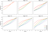 |
Fig. B.1 Curve of growth for the Ca line at 8542 Å. Same as Figure 7 but for Ca 8542 Å. |
| In the text | |
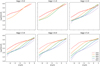 |
Fig. B.2 Curve of growth for the Ca line at 8662 Å. Same as Figure 7 but for Ca 8662 Å. |
| In the text | |
Current usage metrics show cumulative count of Article Views (full-text article views including HTML views, PDF and ePub downloads, according to the available data) and Abstracts Views on Vision4Press platform.
Data correspond to usage on the plateform after 2015. The current usage metrics is available 48-96 hours after online publication and is updated daily on week days.
Initial download of the metrics may take a while.