| Issue |
A&A
Volume 684, April 2024
|
|
|---|---|---|
| Article Number | A81 | |
| Number of page(s) | 11 | |
| Section | Planets and planetary systems | |
| DOI | https://doi.org/10.1051/0004-6361/202348916 | |
| Published online | 05 April 2024 | |
Quantitative grain size estimation on airless bodies from the negative polarization branch
II. Dawn mission targets (4) Vesta and (1) Ceres
1
Korea Astronomy and Space Science Institute (KASI),
776 Daedeok-daero, Yuseong-gu,
Daejeon
34055, Republic of Korea
e-mail: This email address is being protected from spambots. You need JavaScript enabled to view it.
2
Department of Physics and Astronomy, Seoul National University,
Gwanak-ro 1, Gwanak-gu,
Seoul
08826, Republic of Korea
e-mail: This email address is being protected from spambots. You need JavaScript enabled to view it.
3
SNU Astronomy Research Center, Department of Physics and Astronomy, Seoul National University,
Gwanak-ro 1, Gwanak-gu,
Seoul
08826, Republic of Korea
4
Center for Astronomy, University of Hyogo,
407-2 Nishigaichi, Sayo,
Hyogo
679-5313, Japan
5
Japan Spaceguard Association, Bisei Spaceguard Center,
1716-3 Okura, Bisei, Ibara,
Okayama
714-1411, Japan
6
Nayoro Observatory,
157-1 Nisshin, Nayoro,
Hokkaido
096-0066, Japan
7
Department of Astronomy, Graduate School of Science, The University of Tokyo,
7-3-1 Hongo, Bunkyo-ku,
Tokyo
113-0033, Japan
Received:
12
December
2023
Accepted:
10
January
2024
Abstract
Context. Sunlight scattered from the surface of an airless body is generally partially polarized, and the corresponding polarization state includes information about the scattering surface, such as albedo, surface grain sizes, composition, and taxonomic types. Most polarimetric studies on airless bodies thus far have focused on optical wavelengths (λ ≲ 1 µm).
Aims. We conducted polarimetry of two large airless bodies, the Dawn mission targets (1) Ceres and (4) Vesta, in the near-infrared region. We further investigated the change in the polarimetric phase curves over the wavelengths expected from previous works.
Methods. We used the Nishiharima Infrared Camera (NIC) installed at the Nishi-Harima Astronomical Observatory (NHAO) to observe these objects at multiple geometric configurations in the J, H, and Ks bands (λ ~ 1.2–2.3 µm).
Results. Polarimetric parameters were determined and compared with previously reported experimental results. In particular, Vesta exhibits a characteristic change in the negative polarization branch as the wavelength increases to the Ks band, which we interpret as an indication of the dominant existence of D ~ 10–20 µm particles. Our approach is supported by empirical reasoning and coincides well with an independent, theory-driven approach based on thermal modeling.
Conclusions. This work demonstrates how near-infrared polarimetry can be utilized to quantitatively determine the particle size of airless objects. This finding will have important implications for asteroid taxonomy and regolith evolution.
Key words: minor planets, asteroids: general / minor planets, asteroids: individual: (1) Ceres / minor planets, asteroids: individual: (4) Vesta
© The Authors 2024
 Open Access article, published by EDP Sciences, under the terms of the Creative Commons Attribution License (https://creativecommons.org/licenses/by/4.0), which permits unrestricted use, distribution, and reproduction in any medium, provided the original work is properly cited.
This article is published in open access under the Subscribe to Open model. This email address is being protected from spambots. You need JavaScript enabled to view it. to support open access publication.
1 Introduction
The presence of a regolith on an airless body is the result of its initial physical and chemical conditions and specific history of evolution. Among the parameters used to characterize the regolith are grain size, which is related to thermal parameters (Gundlach & Blum 2013), and scattering processes (Hapke 2012), which can change the observable parameters. Thus, quantification of these parameters is one of the important steps in modeling observed quantities. However, the fine nature of grains, as seen with the submicron-scale fine particles retrieved from the Moon (Park et al. 2008), makes it difficult to quantify their sizes, even in this space exploration era.
In our previous work (Bach et al. 2024; Paper I hereafter), our extensive investigation established a methodology for quantifying grain sizes on airless bodies through multiwave-length polarimetry. We focused on exploring the widening-and-deepening (WD) trend within the negative polarization branch (NPB) as triggered by changes in albedo, A(λ), and the size parameter, X ∝ D/λ, where D represents grain size and λ denotes the observation wavelength. We identified two significant effects influencing the NPB across wavelengths. First, as A increases, we observe a WD-like trend for A ≲ 10% and a shallowing trend for A ≳ 10%. Second, regarding D/λ, we found that the NPB stays relatively unchanged for D/λ ≫ 10. However, as λ increases or D/λ decreases, the WD trend starts to appear at D/λ ≲ 5–10. By focusing on the effect of D/λ, we can estimate the particle size that contributes to the scattering process.
Although it is a useful approach, interpreting the WD trend remains challenging due to the potential for a convoluted influence of both albedo and D/λ. Thus, observations of (i) airless objects (ii) covered with fine grains and (iii) exhibiting relatively constant reflectance across visible to near-infrared (NIR) wavelengths are necessary for more reliable interpretations when focusing on the D/λ effect for cases free of the effect of albedo.
The particle size on asteroids is roughly related to the size of the parent asteroid; the larger the asteroid is, the smaller the particle size (Delbo’ et al. 2007; however, see MacLennan & Emery 2022b,a). This is generally understood to be due to the stronger gravity of larger objects (Capria et al. 2014) and/or the shorter lifetime of smaller objects (Delbo et al. 2015). For (1) Ceres (size d ~ 950 km), the presence of ultra-porous fine particles (D ≪ 1 µm) may be required to explain the observations (Li et al. 2019; Schröder et al. 2021; Sect. 4.2.2). Similarly, spectroscopic analyses suggest that (4) Vesta (d ~ 530 km) is predominantly covered with particles of sizes ≲ 20–25 µm (Hiroi et al. 1994; Li et al. 2011; Martikainen et al. 2019), and optical polarimetry has indicated the possibility of a mixture of eucrite grains with sizes >74 µm and <10 µm (Le Bertre & Zellner 1980; also see Sect. 4.2.1).
Therefore, in our study we chose to investigate Ceres and Vesta because (i) they are among the brightest airless objects, (ii) they are likely to possess fine particles that can display the D/λ effect (Paper I), (iii) both have reflectances that suggest they are not subject to a strong albedo effect (Paper I), and (iv) they are targets of the Dawn mission, so a large amount of information is available.
Our NIR polarimetry investigation of airless bodies appears to have commenced nearly simultaneously with that described in Masiero et al. (2022), where the first observations in the J and H bands from UT 2019-03-17 are reported. To the best of our knowledge, Masiero et al. (2022) is the first peer-reviewed publication of NIR polarimetry of airless bodies; it includes our own observations that have been conducted since UT 2019-10-22, at which time we were unaware of their pioneering work. In their work, the albedo and refractive indices, but not the grain size of asteroids, are discussed. In a later study (Masiero et al. 2023), they proposed a qualitative description of the existence of fine-grained inclusions on Barbarian asteroids. Both publications studied wavelengths up to the H band (λ ~ 1.6 µm). We stress that our study is the first NIR polarimetry study of a V-type asteroid (Vesta) and the first polarimetry study of airless bodies at λ > 2 µm (the Ks band), a range that contains critical information (Sect. 4.2.1).
In this study, we conducted a comprehensive investigation utilizing our new data and previous experimental results. The observational circumstances, data reduction methods, and polarimetric parameter finding methods used are summarized in Sect. 2. The results of our observations are presented in Sect. 3. In Sect. 4, we discuss how our results can be interpreted and how the grain sizes of these targets can be obtained. Finally, the appendix provides details on our data reduction and statistical analyses as well as information regarding the data and code availability.
Observing circumstances.
2 Observations and methods
2.1 Instruments and observations
Our observations were conducted using the Nishiharima Infrared Camera (NIC) attached to the 2.0-m Nayuta telescope at the Nishi-Harima Astronomical Observatory (NHAO; 134.3356°E, 35.0253° N, 449 m elevation). The telescope has an altazimuth mount with a f/12.0 focal ratio. The system consists of three detector arrays, each 1024 × 1024 pixel, with two dichroic mirrors such that the three wavelengths are imaged simultaneously. The observed wavelengths are J (central wavelength λ = 1.253 µm with a full width at half maximum Δλ = 0.157 µm), H (λ = 1.632 µm, Δλ = 0.298 µm), and Ks(λ = 2.146 µm, Δλ = 0.313 µm).
In the optical path, a polarimetric mask, a rotating half-wave plate (HWP), and a beam displacer are configured (Takahashi et al. 2018; Takahashi 2019). As a result, two images, ordinary and extraordinary rays (hereafter, o- and e-rays), appear on the same detector at a pixel scale of 0.16″ pix−1. Each image has a size of ~150 × 430 pixels (24″ × 69″) and is displaced horizontally by approximately 200 pixels. Due to the beam displacer, the point spread functions are expected to be different for o- and e-rays
Each set of polarimetric observations consists of four exposures for which with the HWP angle was set to 0°, 45°, 22.5°, and 67.5°, respectively. The four exposures together are denoted as a “set,” with the first two and last two exposures denoted as the q and u subsets, respectively. These parameters are used to determine the normalized Stokes q = Q/I and u = U/I parameters, respectively. We conducted five- and six-night polarimetric observations for Ceres and Vesta, respectively. The observational conditions are summarized in Table 1. On UT2019-11-08, when Vesta was at α = 4.1°, the weather conditions were very unfavorable. This circumstance led to widely varying signal-to-noise ratios (S/N) even between consecutive exposures. Consequently, the uncertainty, particularly in the H-band measurements, was substantially elevated during this period (Table 2).
Polarimetrie data reduction results.
2.2 Data reduction process
The data reduction process follows a similar approach to that of our previous publication (Appendix B of Takahashi et al. 2021), with some modifications implemented using the NICPolpy software1 (Bach et al. 2022). The instrumental gain and readout noise parameters were also updated from Ishiguro et al. (2011). Two polarimetric dome flats were used, one taken on UT 2018-05-07 and the other taken on UT 2020-06-03. For data taken after June 2020, the second master flat was utilized.
The preprocessing steps are as follows: First, artifacts such as vertical and Fourier-like patterns in the frames are removed. Then, standard dark subtraction and flat-fielding are applied. The values at bad pixels, identified using a pre-made bad pixel mask, are replaced with interpolated values from nearby pixels. Each frame is split into two FITS files, which represent the o-ray and e-ray images. Finally, cosmic-ray rejection is performed. Detailed explanations and the implemented algorithms are presented in Bach et al. (2022).
After preprocessing, signal extraction was performed for each exposure. The Stokes parameters were estimated using the ratio method (see, e.g., Bagnulo et al. 2009), considering each subset of exposures. To ensure the robustness of our polarization degree estimation, we extensively tested our results against multiple signal extraction techniques and outlier rejection schemes (see Appendix A). We also conducted thorough verifications to confirm the stability of our final results against different parameter values used in preprocessing, such as those related to artifact removal, the use of different flats, bad-pixel interpolation, and cosmic-ray rejection parameters. These methods only marginally changed the intermediate results, such that the final results (i.e., those describing the polarimetric parameters) do not vary beyond the measurement uncertainty range.
2.3 Polarization parameter calculation
The polarization degree of solar system objects is often described by the properly rotated polarization degree (Lyot 1929):
 (1)
(1)
where P is the total linear polarization degree, θr is the position angle of the strongest electric vector relative to the normal vector of the scattering plane (e.g., 0 or 180° indicates it is normal to the scattering plane), and I⊥ and I|| denote the measured intensities of scattered light along the directions perpendicular and parallel to the scattering plane, respectively.
The curve describing this phenomenon as a function of the phase angle (light source-target-observer angle; α := 180° − scattering angle), Pr(α), is denoted the polarization phase curve (PPC). A PPC at small α can be expressed with a three-parameter linear-exponential function (Muinonen et al. 2002; Kaasalainen et al. 2003):
 (2)
(2)
for free parameters θ1,2,3. The inversion angle α0 can be solved numerically from Pr(α0) = 0, as in Gil-Hutton (2017).
We emphasize that the three parameters used above are eventually converted to polarimetric parameters of interest, for example the polarimetric slope  , inversion angle α0, αmin and Pmin = Pr(αmin). By rearranging the equation, we can generate the fitting parameters with more intuitive meanings and facilitate subsequent statistical analyses of the parameters:
 (3)
(3)
where k [°] is a scale parameter. Having rearranged the equations such that two out of the three fitting parameters (h, α0) are the ones of interest, the error analyses become much more straightforward. Importantly, the function in Eq. (3) describes the identical curve as in Eq. (2). Furthermore, we can obtain αmin through the condition P′r(α = αmin) = 0 as follows:
 (4)
(4)
Therefore, four important parameters, h, α0, αmin, and Pmin = Pr (αmin), are obtained.
3 Results
3.1 PPC of targets
The polarization degrees derived from our data are summarized in Table 2. These polarization degrees (P) are obtained using the formula  , where q and u are the instrumental polarization efficiency and the position-angle corrected values, respectively (Takahashi 2019). To calculate the uncertainties in q and u, we first computed the weighted average and its uncertainty,
  , where σi is the uncertainty of the i-th data point. The final uncertainties, dq and du, were determined as the larger value recorded between the weighted average uncertainty and the standard error (i.e., the sample standard deviation divided by the square root of the number of samples). Because the position angle of the scattering plane at the time of observation has negligible uncertainty, dθP = dθr. For dPr, we applied error propagation to Eq. (1), while neglecting the covariance between dP and dθr. The maximum value between this propagated uncertainty and dP is obtained as dPr.
Notably, these uncertainties are comparable to the standard error from the central limit theorem, which is inherently much less than the random scatter (standard deviation of data points or the error bar of a single data point) by a factor of  . In their work, Masiero et al. (2023) accounted for this discrepancy by quadratically adding 0.1 %p scatter to their reported dPr values. Additionally, these uncertainties do not include systematic errors (see Appendix B).
As shown in Table 2, we have confirmed that our θr values are generally close to integer multiples of 90°, as expected from symmetry considerations (Lyot 1929; Cellino et al. 2018). Consequently, cos(2θr) ≈ 1. The extreme exception is Vesta at α = 22.5°, where its polarization degree is near zero; thus, θr is not well defined in this particular case. This finding strongly supports the credibility of our data reduction process. Conversely, we can further utilize our θr values of asteroids to measure the instrumental offset (assuming it must be an integer multiple of 90°) when |Pr| is large. For example, using Ceres data at α = 8.6°, we find that the instrumental position angle offset is <2° for all the filters, which is consistent with Takahashi (2019).
The PPCs for Ceres and Vesta are derived and plotted in Fig. 1. For Ceres, two datasets from a previous publication were included (Masiero et al. 2022). We have overplotted these data in the figures, and the results of our observations closely match the corresponding fitting curves. The shaded regions in the figures represent the approximate 1σ range of the fitting models obtained from Monte Carlo (MC) simulations (Appendix C).
In Fig. 2, we present the same data and curves as shown above, but with the inclusion of optical observations from Lupishko (2022)2 and Bendjoya et al. (2022). For Vesta, we also used the data provided in Cellino et al. (2016), which were not included in previous datasets (at eight different αs), after taking the nightly median (3-σ-clipped). When fitting the optical data, we used data only when the reported error bar for the polarization degree was <0.15 %p; we neglected any uncertainties in the data because of the inhomogeneity in the data across multiple sources. Notably, we expect optical data to have higher uncertainties. For example, a few noisy Ceres data points near α0 affect the h values (i.e., they have high leverage values). Finally, we excluded data points with >0.25 %p deviation from the fitting line. We explored various processing methods, such as using only the data with available uncertainties, changing the error bar threshold, and/or adding a range of uncertainties (0.02–0.5 %p) in quadratures based on different criteria. The fitted polarimetric parameters change for these optical data; thus, the uncertainties of these parameters were difficult to quantify; however, our main results, discussed in Sect. 4, were not affected by these variations.
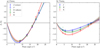 |
Fig. 1 PPCs of two objects in the NIR data from this study (star) and a previous publication (circle; Masiero et al. 2022). The solid lines are the least-square solutions, and the shaded areas show the MC 1σ bounds. |
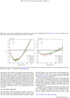 |
Fig. 2 Same as Fig. 1 but with optical data (Lupishko 2022). The solid lines are the least squares solutions for each wavelength range of the data, and the cross markers (“×”) indicate the masked data points. |
3.2 Polarimetric parameters
The final fitting results are presented in Table 3. The best fit parameter values are the least-square solution, while the error bars are from the 16th and 84th percentiles of the MC samples.
The MC median is very close to that of the least-square solutions, differing by only ≪ 1σ. For Ceres, we also included data from Masiero et al. (2022). More detailed information on the MC simulation is provided in Appendix C.
Several observations can be made from the abovementioned results: (i) the Ceres NPB does not appear to vary significantly with wavelength, and (ii) Vesta shows a clear trend of changing the NPB with wavelength, including a deepening trend in the Ks band. The interpretations and discussions of these results are presented in Sect. 4.
In addition to the polarimetric parameters, the albedo value of the objects plays a crucial role in understanding their properties. To calculate the albedos of Ceres and Vesta, we utilized the catalog of visible to NIR reflectance spectra3, which covers λ ~ 0.45–2.5 µm, along with the filter profile information of the NIC. We performed trapezoidal numerical integration of the spectra using the filter profiles (but ignoring the reflectance and transmission of the dichroic mirrors) and then converted the integrated value back to the physical albedo. This process implicitly assumes that the spectrum used is the same at α = 0°, implying that the backscattering amplitude is assumed to be identical over the wavelength range. The geometric albedo at a wavelength of λ = 0.55 µm (FC2 filter of the Dawn spacecraft) was adopted as p0.55 μm = 0.094 ± 0.007 for Ceres (Ciarniello et al. 2017) and 0.38 ± 0.04 for Vesta (Li et al. 2013). The resulting albedo values and their uncertainties are summarized in Table 4. For the optical observations, we used a uniform filter profile spanning the wavelength range with 0.01 µm bezels (e.g., for 0.45–0.60, wavelengths from 0.45 + 0.01 = 0.46 µm to 0.60–0.01 = 0.59 µm). We used albedos only for λ > 0.4 µm.
For comparison, the figures in Paper I present Ceres and Vesta overlaid on various parameter spaces along with laboratory samples and other asteroids in the albedo–Pmin−h−α0 space. Among these parameters, the Umov laws (h−albedo and Pmin− albedo relations) are shown in Figs. 3–5 of Paper I. For optical wavelengths, rotational variations in amplitude <0.1 %p and the Umov law were studied for Vesta (Cellino et al. 2016). However, we did not consider the rotational variation.
In the Pmin−α0 space (Fig. 7 in Paper I), the change in the location of Vesta, likely starting in the Ks band, is noteworthy. Vesta is near S-complex asteroids (Belskaya et al. 2017) but moves toward the lunar fine region in the Ks band. For the Moon, most regions exhibit a WD trend (because of the albedo effect and/or D/λ effect). A similar WD trend is also observed for Vesta. In contrast, the NPB shows almost no change in Ceres in the Pmin−α0 space.
Fitting results.
Geometric albedos and uncertainties.
4 Discussion
4.1 The Umov laws (h, Pmin, and albedo)
The h-albedo and Pmin–albedo relations are shown in Figs. 3–5 of Paper I. First, the two objects in the NIR region roughly follow Umov laws. To the best of our knowledge, this is the first report on the location of small airless bodies in these parameter spaces at NIR wavelengths, even though further investigation is needed to verify its generality. Second, Vesta changes its location toward the fine particles (small D/λ) in both parameter spaces, which supports the existence of fine particles on Vesta. As mentioned, the Ceres h optical data are susceptible to a few noisy data points near the inversion. Ceres also shows a noticeable trend of increasing h (but not Pmin) only in the Ks band, while the albedo and Pmin remain nearly constant.
4.2 Pmin − α0 space
The NPB of Vesta clearly shows a trend of WD increasing λ, as shown in, for example, Fig. 6 of Paper I. However, Ceres stays at a fixed location over the investigated wavelengths (<0.5 µm to >2 µm). We therefore discuss the particle sizes on these objects based on these observations.
4.2.1 Determining Vesta's particle size
Vesta has albedo ≫10% all over the wavelengths of interest (Table 4), which allows us to conclude that WD of the NPB by the albedo effect (Paper I) is unlikely. Therefore, the likely cause is the effect of D/λ. We argue that D/λ ~ 5–10 is reached in the H or Ks band (λ ~ 2 µm), so Vesta is likely covered with particles of size D ≳ 10–20 µm. Finer particles (~ 1 µm) should not dominate the surface; if they do, that indicates that we must have detected a WD trend (or a narrowing-and-deepening trend) in the UV-to-J band observations.
This particle size is consistent with previous speculations. Most importantly, Le Bertre & Zellner (1980) was one of the first studies to investigate optical NPB to determine the grain size of Vesta. After testing multiple Howardite, eucrite, and diogenite (HED) meteoritic samples, ≲20 µm particles were found to be necessary to reproduce the observed α0 of Vesta. However, finer particles resulted in too high an albedo4 compared to Vesta’s albedo known at the time (0.22; Morrison 1977; Zellner et al. 1977). Because of this mismatch, coarse particles are required to reduce the albedo. Finally, taking all these factors into account, they concluded that the eucrite Bereba sample of coarse particles (>76 µm) covered with fine (<10 µm) particles (denoted Bereba B) can match both the α0 and albedo at the same time.
However, based on the Dawn mission, Vesta’s geometric albedo is updated to pV = 0.42 (Li et al. 2013), and the phase function in the F2 filter (Fig. 19a in Li et al. 2013) shows that the albedo at α = 5° is ≳0.3, compared to earlier values 0.22. Thus, the logic that led Le Bertre & Zellner (1980) to a large fraction of coarse particles should be reconsidered. Instead, the updated data may support a larger fraction of finer particles, which is consistent with our results.
Later, Hiroi et al. (1994) used an independent method (reflectance spectrum analysis) and found that the finest particle size (<25 µm) of HED powders best reproduced the Vesta 0.3–2.6 µm spectra. Hence, they also concluded that very fine (<25 µm) particles are necessary to explain Vesta’s reflectance spectrum. Recently, Li et al. (2011) reached a similar conclusion that a single, fine-grained Howardite with a size of <25 µm suitably fits the Hubble Space Telescope, Swift, and International Ultraviolet Explorer (IUE) observations. In addition, Martikainen et al. (2019) showed that, using ray-optic simulation calculations, Vesta’s surface is dominated (>75%) by fine Howardite particles of size <25 µm.
Finally, utilizing the thermal conduction modeling algorithm (MacLennan & Emery 2022b), we found two solutions for Vesta, D ≲ 10 µm and D ≳ 50 µm, both of which require a porosity ≳80%. Remarkably, this theoretical modeling, independent of polarimetry, yielded results that align quite closely with our findings. The slight disparity between our findings and those of the theoretical thermal model can be attributed to multiple factors, including that polarimetry detects only the topmost layer of the scattering process, whereas thermal modeling probes are significantly deeper (on the order of the thermal skin depth, which varies from the millimeter scale to as high as the meter scale).
Combining the lower bound from our study and the upper bounds from previous works, we propose that Vesta is covered with D ~ 10–20 µm particles.
4.2.2 The case of Ceres
Because Ceres shows no change in the Pmin−α0 space, one could argue that D/λ ≫ 10 until the Ks band (D ≫ 20 µm). On the other hand, as noted in Paper I, the narrowing-and-deepening (ND) trend is not clearly detected across the literature, because of the inherent practical difficulty. Moreover, further experiments are needed to investigate when the ND trend stops and how this trend can differ at low albedos (A ≲ 10%). Therefore, another possible hypothesis is that the fact that D/λ ≪ 1–2, even at the shortest wavelength (i.e., D ≪ 0.5–1 µm), is the cause of Ceres’s behavior.
From the Dawn observations, the wavelength dependence of the single-particle phase function is found (Li et al. 2019). They found that a considerable fraction of ≲ 1 µm particles can explain this dependence. Some regions near young impact craters on Ceres show blue spectra (Schröder et al. 2017). Later, Schröder et al. (2021) showed that these locations are likely to contain hyperporous, foam-like phyllosilicate structures, which effectively act as Rayleigh scatterers with a characteristic filament size ≪1 µm and filament separation ≫1 µm. These can support the small particle scenario.
Utilizing a thermal modeling algorithm similar to Vesta (MacLennan & Emery 2022b), we found two solutions, D ≲ 2 µm and D ≳ 30 µm, both with porosities >80% (cross-checked with MacLennan, E. 2023, priv. comm.). We can reject neither the small nor large particle scenarios. However, we again stress that both possible scenarios from this work and thermal modeling, which are completely independent approaches, expect for surprisingly consistent particle sizes.
Because the NPB behavior of Ceres seems to be typical of C-complex objects (Masiero et al. 2022), further exploration of the change in the NPB for low-albedo materials is key for understanding C-complex objects. Moreover, these findings will naturally deepen our understanding of the thermal behavior of these materials by cross-validating both approaches.
Finally, we note that Ceres’s location in the h-albedo space is changed in the Ks band. This may indicate the existence of a fine structure. However, as shown in Paper I, the deviation for low-albedo (A ≲ 10%) materials has been investigated less than that for higher-albedo materials; thus, further investigations are needed.
4.3 Revisiting several previous works
Belskaya et al. (1987) demonstrated similar trends in Pmin for both Vesta and (16) Psyche across UBVRI bands, despite differences in their reflectances. A later study showed that S- and M-types generally exhibit the opposite trend to that of the Umov law, which posits an inverse correlation between the polarization degree (|Pmin|) and albedo (Belskaya et al. 2009). This finding suggested that the Umov law is not the sole mechanism influencing the shape of the NPB. This trend aligns with the WD trend, while the trend for low-albedo objects (WD-like as albedo increases; Paper I) is also possible5. This finding highlights the importance of Vesta because it has a sufficiently high albedo (Table 4) and allows us to rule out the presence of the albedo effect with a higher confidence.
Bagnulo et al. (2015) mentioned that “the Umov law may be violated” based on the spectropolarimetry of the Barbarian asteroids. They found that (7) Iris and (599) Luisa showed that |Pr(λ; α)| decreased with increasing reflectance, which matches the Umov law, while (236) Honoria showed the opposite trend over λ. They further discussed that the difference in polarimetric colors between Honoria and Luisa is puzzling because both are Barbarians; over these wavelengths, the NPB becomes deeper for Honoria and shallower for Luisa.
We emphasize that if the ND trend is present on these Barbarian asteroids, this is an expected behavior. Honoria and Luisa were observed at α = 7.1° (where Pr gets deeper with increasing λ) and α = 26.9° (slightly below α0, where Pr gets shallower with increasing λ), respectively. Indeed, Masiero et al. (2023) found that L-types show an ND trend over the wavelength in the NIR region.
We agree with their interpretation that the NPB of L-type asteroids is affected by fine grains (D/λ < 1–2). This example hints that the Umov law should be applied with care; for example, one may use h or Pmax (Pmin may be less accurate). It is natural that the inverse Umov law or even the independence of the polarization degree from the wavelength may be observed at certain phase angles. Similarly, the change in NPB for S-types may indicate the presence of smaller particles on them, which may be related to the explanation in Hasegawa et al. (2019). A possible test observation would include NIR polarimetry of Q-types because they would not show a clear WD trend as S-types if the WD trend was indeed driven by fine particles.
In Kwon et al. (2023), an anticorrelation was found between a0 and the asteroid diameter of the C-complex. These authors mentioned that this contradicts the fact that larger asteroids may contain finer particles. We hypothesize that this can also be interpreted as the ND trend being observed: the C-complex objects with diameters d > 100 km already possess fine particles that can induce the ND trend, so α0 decreases as D decreases (i.e., a decreasing a0 increases d). We admit that this should be considered a primitive hypothesis because there was no clear ND trend observed for a single object.
5 Conclusions and future work
In this work, we have shown that NIR polarimetry can be used as a tool for quantifying grain size. We observed two of the largest airless bodies, (1) Ceres and (4) Vesta, which are Dawn mission targets. These airless objects were chosen because they are very likely to possess very fine particles on their surfaces; hence, D/λ is expected to be small enough to indicate the change in the NPB over NIR wavelengths. The data were processed with extreme care to achieve the best possible accuracy. Conclusions from this work are summarized as follows:
The Umov laws (slope–albedo and Pmin–albedo correlations) for airless bodies apparently hold at NIR wavelengths. At the longest wavelengths, however, they begin to deviate, which is attributed to the decreased D/λ;
Vesta showed a characteristic change in the NPB when λ was increased to the H and Ks bands (λ ≳ 2 µm). Combining our data with those of previous studies, we find that the optically significant grain size on Vesta is ~ 10–20 µm. This finding agrees with that of multiple previous independent reports. To the best of our knowledge, this report is the first quantification of grain size on airless bodies based on NIR polarimetry;
For Ceres, there was no significant change in the NPB (Pmin, α0). This indicates the potential existence of either very fine particles (D ≪ 1 µm) or large particles (D ≫ 20 µm).
Our empirical estimation of particle sizes using multiwave-length polarimetry strongly aligns with an independent theoretical modeling approach (thermal modeling). This successful congruence between the two methodologies represents a significant cross-validation of the two scientific approaches.
Because Vesta is known to have high heterogeneity in terms of albedo and composition (Reddy et al. 2012), disk-resolved polarimetry of Vesta near αmin can reveal valuable hints about the parameters that change the NPB. A change in the polarimetric slope (h) of Ceres in the Ks band may provide important information about its surface structure. A further experimental exploration of darker materials, for example using the samples from (101955) Bennu obtained by OSIRIS-REx (Lauretta et al. 2017) or (162173) Ryugu by Hayabusa 2 (Nakamura et al. 2023), may further advance our understanding of the case of dark C-complex and related objects.
Acknowledgements
This work was supported by a National Research Foundation of Korea (NRF) grant funded by the Korean government (MEST; No. 2023R1A2C1006180). Y.P.B. would like to thank Eric MacLennan for helpful cross-checking of the grain size calculations and engaging discussions about Ceres. The authors want to thank Joseph Masiero for providing constructive comments as a referee.
Appendix A Details of the polarimetry
A set of observations contains four exposures at HWP angles of θ = 0°, 45°, 22.5°, and 67.5°. In this work, we call the first two and the last two the q-subset and u-subset, as they are used to obtain Stokes q : = Q/I and u : = U/I, respectively. For each subset, four intensities were measured (the o- and e-ray for each exposure). The measured intensities of the target are a for the o-ray of the first frame, b for the e-ray of the first frame, c for the o-ray of the second frame, and d for the e-ray of the second frame. The Stokes parameter s (either q or u) is estimated as
 (A.1)
(A.1)
where
 (A.2)
(A.2)
To obtain a to d, we used simple circular aperture photometry since the point-spread function of the NIC is nearly circular. We always fixed the sky-estimating region as a circular annulus with inner and outer radii of 70 and 90 pixels, respectively. This is determined so that it is large enough to avoid any flux from our object even when the target is the brightest throughout our whole observational period. For some selected cases, by changing this annulus we obtain a result that changes less than the final 1σ error bar for the Pr value. The sky value was estimated based on the SExtrator-like algorithm (Bertin & Arnouts 1996). First, 3-sigma clipping was performed for a maximum of 5 iterations to reject extreme pixel values. Then, for the sigma-clipped mean, median, and standard deviation (ssky), the modal value is msky = (2.5 × median) − (1.5 × mean) if (mean − median)/ssky ≤ 0.3; otherwise, msky = median. This is a slightly modified version of the widely used mode estimation from a unimodal distribution (Doodson 1917). Since the size of the final image for each of the o- and e-rays is 130 × 410 pixels (Bach et al. 2022), the regions outside these regions are regarded as blank pixels in sky estimation.
In addition to a to d, we also calculate their uncertainties by
![Mathematical equation: ${\rm{\Delta }}a = \sqrt {{{\left( {1 + {\delta _F}} \right)\left( {a + {m_{{\rm{sky}}}}} \right)} \over g} + \pi r_{{\rm{ap}}}^2\,\left[ {{{\left( {{{{R_e}} \over g}} \right)}^2} + s_{{\rm{sky}}}^2} \right]} ,$](/articles/aa/full_html/2024/04/aa48916-23/aa48916-23-eq41.png) (A.3)
(A.3)
and similar for b to d. Here, δF is a factor for coping with the uncertainty in flat fielding, which we fixed to 0.02 (Stetson 1987, and DAOPHOT4 uses the default 0.0075, Stetson, P. B. 2023, priv. comm.), g is the gain factor of the detector in electron/ADU (Bach et al. 2022), rap is the aperture radius (Appendix A.2), and Re is the readout noise in the electron unit. The S/N is calculated as S/Na = a/Δa, and so on. The uncertainty in Stokes s is
 (A.4)
(A.4)
Appendix A.1 Effect of outliers
For each subset, we calculate four S/N values: {S/Na, S/Nb, S/Nc, S/Nd}. Then, the minimum of these is saved as the representative S/N, and the peak-to-peak difference (maximum minus minimum) is called dS/N. Next, we selected sets only if all the following criteria were met:
S/Ns > SNR_min for both s = q and u
S/Ns/dS/Ns > SNR_factor for both s = q and u
Δs < ds_max for both s = q and u.
We selected SNR_min = 20, SNR_factor = 5, and ds_max = 0.5%. When we change these, some data points are affected, but the effects on Pmin and α0 are marginal. We introduce this screening method to remove the observations that were made when thin clouds passed through the field of view (i.e., when the S/N was too small or changed rapidly within two consecutive exposures). The choice of these parameters generally does not change the Pr value at all (much smaller than the 1σ error bar). For the case of the H band of Vesta on UT 2019-11-08, we found that different combinations of SNR_min and SNR_factor (e.g., 30 and 4) can change it by the order of the 0.1–0.2 %p level, but this change is still within the order of the error bar. Even if this data point at α = 4.1° is very uncertain, it is far from αmin and α0, so the estimated locations of Vesta in the Pmin−α0 space are not affected.
After this first screening, we applied the generalized extreme Studentized deviate test (Rosner 1983, implemented in scikit-posthocs by Terpilowski 20196) to remove an unknown number of outliers in the q-u plane. This rejection was based on the distance of the data points with respect to the average point in the q-u plane, with a significance level of 0.95. We did not find a strong deviation from the final results due to this process.
Appendix A.2 Effect of aperture modes
Changing the centroiding algorithm can change the total flux by a small amount, but this change is much smaller than the change in the sky modal values. Thus, the remaining important factor that can affect the final result is how we select the aperture radius. We tested multiple algorithms to determine the best aperture size for estimating the incident flux.
Considering that the typical full width at half maximum of NIC is approximately 15 pixels, we first calculated the aperture sum using a fixed aperture radius of rap = 25, 30, 35 and 40 pixels (denoted as codes 25, 30, 35, and 40). Since the full widths at half maximum clearly vary each night, this results in either a loss of flux (small radius) or a larger scatter (large radius). What makes this more challenging is that we sometimes defocused the image intentionally to avoid saturation. Thus, a single-aperture size is sometimes not appropriate, even over a single night.
Another possible method is to change the aperture size for each subset. Since each exposure results in two images of the target (the o-ray and the e-ray), there are four images. For each of these images, we obtained the modal pixel values as a function of the radial distance from the centroid of our target (for distances of 5 to 60 pixels). The modal values were calculated using an algorithm identical to that used for sky modal value estimation by using a circular annulus of 1 pixel thickness. Then, we selected the minimum radius that has a modal value > msky + 1 × ssky (denote it rap0). If the object is too faint and no such radius exists, we use rap0 = 5. For the four rap0 values obtained in this way, we can choose a fixed rap for all four images using either the minimum or maximum of the rap0’s (denoted as code min and max, respectively). Finally, the point spread function of the o- and e-rays is expected to be different for NIC since it uses a beam displacer. Thus, we can also try using separate rap for the o-ray and the e-ray, rapo and rape, respectively. rap,o|e can be the smallest among the two rap0,o|e values (denoted as code minoe) or the largest (maxoe).
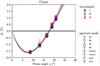 |
Fig. A.1 Effect of the choice of aperture size in the Ceres case. Different colors correspond to different bands (J, H, and Ks), while different markers correspond to different aperture modes. The solid lines are linear-exponential fits to each band and aperture mode. |
For example, if we assume the rap0 values are 15 and 16 for the first frame and 17 and 18 for the second frame (o- and e-ray, respectively), under our notation rap would be 25 for the 25 code, regardless of rap0 values; rap = 15 for min; rap = 18 for max; rap,o|e = 15| 16 for minoe; and rap,o|e = 17| 18 for maxoe.
We find our final results to be extremely robust to all of these different aperture models (Figs. A.1 and A.2). For Vesta, (i) the inversion angle a0 might be slightly uncertain, especially because there are no data at α > α0, and (ii) the error bar of the smallest α observation (UT2019-11-08) varies depending on the aperture mode. However, as seen from the figures, this does not change the logic of this paper. All the main results presented in this work are derived using the min aperture model.
Appendix B Possible systematic uncertainties
As usual in any observation or experiment, our observational results may be subject to systematic offsets. Here, we describe possible underlying factors. According to our observations, there are two potential sources of systematic offsets: additive instrumental offsets in terms of the polarization degree and position angle.
An investigation conducted by Takahashi et al. (2018) demonstrated that the instrumental polarization degree offset (the so-called instrumental polarization degree) is very small for NIC and is effectively zero within the uncertainty level. The maximum offset occurs in the Ks band, with values of (qoff, uoff) = (−0.02 ± 0.30, −0.07 ± 0.31) %p, where the error bars represent the standard deviation of 180 sets of three unpolarized standard stars. For all the other cases, the offsets are ≤ 0.03 %p. Therefore, the instrumental polarization degree offset is expected to be at most of the same order as the random scatter (dPr). Thus, we decided to skip this offset correction since it is negligible compared to random scatter.
The systematic offset in the instrumental position angle is estimated to be on the order of a few degrees (Takahashi 2019). The effect of this offset on Pr is also expected to be very small. According to Eq. (1), an extreme systematic offset of Δθr = 10° from θr = 0° would result in only ΔPr/Pr = 0.06. Since the actual offset is Δθr ~ 1° and our data are |Pr| < 2 %, we expect ΔPr ≪ 0.1 %p for all our data.
Another potential source of systematic offset comes from the polarization efficiency, peff. As mentioned by Takahashi (2019), the NIC has an efficiency of peff > 0.9, with values of approximately 100% within the error bars: (98, 95, 92) ± (6, 7, 12)% for the J, H, and Ks bands, respectively. We applied these efficiency corrections to our data. The uncertainties provided are the standard deviations, not the standard errors. Unlike the previous two offsets discussed, peff is generally considered to have a multiplicative effect (Akitaya et al. 2014), as it is caused mainly by the imperfect extinction ratio of the polarizer. Therefore, it linearly affects Pr in Eq. (1). This means that Pr might be systematically offset (multiplied) by ≲ 0.1 %p in our case (Table 2). We emphasize, however, that this does not affect our overall logic.
In the work by Masiero et al. (2022), they also found a hint of instrumental systematic offset with ΔP = +0.042 and +0.088 %p in the J and H bands, respectively. In their work, they used an empirical law (Serkowski et al. 1975) with the assumption that the maximum polarization occurs at 0.55 µm for calibrating the instrumental offsets. Likely stemming from the different calibration processes, our data are slightly offset from theirs (e.g., 0.1 %p level near αmin for Ceres). We again emphasize that this difference does not affect our discussion.
Appendix C Monte Carlo simulation and uncertainties
We adopted the Markov chain MC package emcee (Foreman-Mackey et al. 2013, 2019) with an affine-invariant ensemble sampler for our fitting process. We first calculated the least-square solution for each object and each filter. The priors for h, α0, and k in Eq. (3) are chosen to be uniform in the range of h ∈ [0.01,10] (in %/°), α0 ∈ [10, 30], and k ∈ [10−5, 100] (both in degrees). The initial positions for 32 chains are randomly selected near this position in the three-dimensional parameter space. Then, with the stretch-move algorithm, 3000 samples per chain are drawn. The first 1000 samples from all the samples were discarded; thus, 64000 MC samples were left per object per filter. The αmin and corresponding Pmin values are calculated for each sample after the sampling process (Eq. (4)). We assumed that the uncertainty of each observation was purely Gaussian, so the log-likelihood method used the usual figure of merit:
 (C.1)
(C.1)
Here, Pr,obs,i and dPr,obs,i are the observed polarization degree of the ith data point and its uncertainty, respectively. The log posterior probability function is calculated by adding the log of the prior function to ℒ.
Then, we discarded samples if they were outside any of the +5σ ranges of the three parameters (the asymmetry σ for each parameter was calculated from the 16th, 50th, and 84th percentiles of the MC samples). This process discarded up to a few hundred samples. We checked that the randomness of the MC sampling did not change the results by more than 0.1σ.
To obtain the 1σ uncertainty range of the curves in Figs. 1 and 2, we first calculated the log-likelihood of each sample and converted it to the usual; χ2 statistic (χ2 = −2ℒ). Then, the samples with
 (C.2)
(C.2)
are selected. Here, min{χ2} is the lowest χ2 value of all the samples (which should be nearly identical to that of the least-square solution), and; is the percent point function, that is to say, the inverse of the cumulative distribution function of the;χ2 distribution of the degrees of freedom v. The constant 0.6827 is selected specifically for the “1σ” range. In our case, Eq. (3) contains three parameters of interest, so v = 3. Model parameters within the 1σ uncertainty range were selected in the one-tailed test, which is the method suggested in Press et al. (2007, Sect. 15.6)7.
Appendix D Data and code availability
We obtained approximately 8 GB and 13 GB of raw data for Ceres and Vesta, respectively. There are approximately 16 GB of dome flats, and some standard star observations are approximately 16 GB. Then, the preprocessed data (levels 1-4, Bach et al. 2022) are approximately 3 times the total size (100+ GB of data). Due to the large size of the total dataset, we only uploaded (i) the raw (level 0) data of Ceres and Vesta, (ii) the final (level 4) data of Ceres and Vesta, (iii) the corresponding log files produced from NICpolpy (Bach et al. 2022), (iv) the used calibration frames, (v) the automatically generated observational logs in PDF format and (vi) the skymonitor record videos. They are available via Zenodo8. Part of the codes and data used for this publication are available via GitHub9
References
- Akitaya, H., Moritani, Y., Ui, T., et al. 2014, SPIE Conf. Ser., 9147, 91474O [NASA ADS] [Google Scholar]
- Bach, Y. P., Ishiguro, M., Takahashi, J., & Geem, J. 2022, Stars and Galaxies, 5, 4 [NASA ADS] [Google Scholar]
- Bach, Y. P., Ishiguro, M., Takahashi, J., et al. 2024, A&A, 684, A80, (Paper I) [NASA ADS] [CrossRef] [EDP Sciences] [Google Scholar]
- Bagnulo, S., Landolfi, M., Landstreet, J. D., et al. 2009, PASP, 121, 993 [Google Scholar]
- Bagnulo, S., Cellino, A., & Sterzik, M. F. 2015, MNRAS, 446, L11 [Google Scholar]
- Belskaya, I. N., & Shevchenko, V. G. 2000, Icarus, 147, 94 [NASA ADS] [CrossRef] [Google Scholar]
- Belskaya, I. N., Lupishko, D. F., & Shakhovskoi, N. M. 1987, Sov. Astron. Lett., 13, 219 [Google Scholar]
- Belskaya, I. N., Levasseur-Regourd, A.-C., Cellino, A., et al. 2009, Icarus, 199, 97 [Google Scholar]
- Belskaya, I. N., Fornasier, S., Tozzi, G. P., et al. 2017, Icarus, 284, 30 [Google Scholar]
- Bendjoya, P., Cellino, A., Rivet, J. P., et al. 2022, A&A, 665, A66 [NASA ADS] [CrossRef] [EDP Sciences] [Google Scholar]
- Bertin, E., & Arnouts, S. 1996, A&AS, 117, 393 [NASA ADS] [CrossRef] [EDP Sciences] [Google Scholar]
- Capria, M. T., Tosi, F., De Sanctis, M. C., et al. 2014, Geophys. Res. Lett., 41, 1438 [NASA ADS] [CrossRef] [Google Scholar]
- Cellino, A., Ammannito, E., Magni, G., et al. 2016, MNRAS, 456, 248 [Google Scholar]
- Cellino, A., Bagnulo, S., Belskaya, I. N., & Christou, A. A. 2018, MNRAS, 481, L49 [NASA ADS] [CrossRef] [Google Scholar]
- Ciarniello, M., De Sanctis, M. C., Ammannito, E., et al. 2017, A&A, 598, A130 [NASA ADS] [CrossRef] [EDP Sciences] [Google Scholar]
- Delbo’, M., dell’Oro, A., Harris, A. W., Mottola, S., & Mueller, M. 2007, Icarus, 190, 236 [CrossRef] [Google Scholar]
- Delbo, M., Mueller, M., Emery, J. P., Rozitis, B., & Capria, M. T. 2015, in Asteroids IV, eds. P. Michel, F. E. DeMeo, & W. F. Bottke (Tucson: University of Arizona Press), 107 [Google Scholar]
- Doodson, A. T. 1917, Biometrika, 11, 425 [Google Scholar]
- Foreman-Mackey, D., Hogg, D. W., Lang, D., & Goodman, J. 2013, PASP, 125, 306 [Google Scholar]
- Foreman-Mackey, D., Farr, W., Sinha, M., et al. 2019, J. Open Source Softw., 4, 1864 [NASA ADS] [CrossRef] [Google Scholar]
- Gil-Hutton, R. 2017, in ACM (Asteroid, Comets, Meteors) 2017, Montevideo, Poster 1.d.17 [Google Scholar]
- Gundlach, B., & Blum, J. 2013, Icarus, 223, 479 [Google Scholar]
- Hapke, B. 2012, Theory of Reflectance and Emittance Spectroscopy (Cambridge University Press) [Google Scholar]
- Hasegawa, S., Hiroi, T., Ohtsuka, K., et al. 2019, PASJ, 71, 103 [NASA ADS] [CrossRef] [Google Scholar]
- Hiroi, T., Pieters, C. M., & Takeda, H. 1994, Meteoritics, 29, 394 [NASA ADS] [Google Scholar]
- Ishiguro, M., Takahashi, J., Zenno, T., Tokimasa, N., & Kuroda, T. 2011, Annu. Rep. Nishi-Harima Astron. Observ., 521, 13 [Google Scholar]
- Johnson, P. E., Kemp, J. C., Lebofsky, M. J., & Rieke, G. H. 1983, Icarus, 56, 381 [NASA ADS] [CrossRef] [Google Scholar]
- Kaasalainen, S., Piironen, J., Kaasalainen, M., et al. 2003, Icarus, 161, 34 [Google Scholar]
- Kwon, Y. G., Bagnulo, S., & Cellino, A. 2023, A&A, 677, A146 [NASA ADS] [CrossRef] [EDP Sciences] [Google Scholar]
- Lauretta, D. S., Balram-Knutson, S. S., Beshore, E., et al. 2017, Space Sci. Rev., 212, 925 [Google Scholar]
- Le Bertre, T., & Zellner, B. 1980, Icarus, 43, 172 [NASA ADS] [CrossRef] [Google Scholar]
- Li, J.-Y., Bodewits, D., Feaga, L. M., et al. 2011, Icarus, 216, 640 [NASA ADS] [CrossRef] [Google Scholar]
- Li, J.-Y., Le Corre, L., Schröder, S. E., et al. 2013, Icarus, 226, 1252 [CrossRef] [Google Scholar]
- Li, J.-Y., Schröder, S. E., Mottola, S., et al. 2019, Icarus, 322, 144 [NASA ADS] [CrossRef] [Google Scholar]
- Lupishko, D. 2022, NASA Planetary Data System, 1, 575 [Google Scholar]
- Lyot, B. 1929, PhD Thesis, Université Pierre et Marie Curie (Paris VI), France [Google Scholar]
- MacLennan, E. M., & Emery, J. P. 2022a, Planet. Sci. J., 3, 263 [NASA ADS] [CrossRef] [Google Scholar]
- MacLennan, E. M. & Emery, J. P. 2022b, Planet. Sci. J., 3, 47 [NASA ADS] [CrossRef] [Google Scholar]
- Martikainen, J., Penttilä, A., Gritsevich, M., Videen, G., & Muinonen, K. 2019, MNRAS, 483, 1952 [CrossRef] [Google Scholar]
- Masiero, J. R., Tinyanont, S., & Millar-Blanchaer, M. A. 2022, Planet. Sci. J., 3, 90 [NASA ADS] [CrossRef] [Google Scholar]
- Masiero, J. R., Devogèle, M., Macias, I., Castaneda Jaimes, J., & Cellino, A. 2023, Planet. Sci. J., 4, 93 [NASA ADS] [CrossRef] [Google Scholar]
- Morrison, D. 1977, Icarus, 31, 185 [NASA ADS] [CrossRef] [Google Scholar]
- Muinonen, K., Piironen, J., Kaasalainen, S., & Cellino, A. 2002, Mem. Soc. Astron. Ital., 73, 716 [Google Scholar]
- Nakamura, T., Matsumoto, M., Amano, K., et al. 2023, Science, 379, abn8671 [NASA ADS] [CrossRef] [Google Scholar]
- Park, J., Liu, Y., Kihm, K. D., & Taylor, L. A. 2008, J. Aerospace Eng., 21, 266 [CrossRef] [Google Scholar]
- Press, W. H., Teukolsky, S. A., Vetterling, W. T., & Flannery, B. P. 2007, Numerical Recipes, 3rd edn. (Cambridge University Press) [Google Scholar]
- Reddy, V., Nathues, A., Le Corre, L., et al. 2012, Science, 336, 700 [NASA ADS] [CrossRef] [Google Scholar]
- Rosner, B. 1983, Technometrics, 25, 165 [Google Scholar]
- Schröder, S. E., Mottola, S., Carsenty, U., et al. 2017, Icarus, 288, 201 [CrossRef] [Google Scholar]
- Schröder, S. E., Poch, O., Ferrari, M., et al. 2021, Nat. Commun., 12, 274 [CrossRef] [Google Scholar]
- Serkowski, K., Mathewson, D. S., & Ford, V. L. 1975, ApJ, 196, 261 [NASA ADS] [CrossRef] [Google Scholar]
- Stetson, P. B. 1987, PASP, 99, 191 [Google Scholar]
- Takahashi, J. 2019, Stars and Galaxies, 2, 3 [NASA ADS] [Google Scholar]
- Takahashi, J., Zenno, T., Saito, T., & Itoh, Y. 2018, Stars and Galaxies, 1, 17 [NASA ADS] [Google Scholar]
- Takahashi, J., Itoh, Y., Matsuo, T., et al. 2021, A&A, 653, A99 [NASA ADS] [CrossRef] [EDP Sciences] [Google Scholar]
- Terpilowski, M., 2019, J. Open Source Softw., 4, 1169 [NASA ADS] [CrossRef] [Google Scholar]
- Zellner, B., Gehrels, T., & Gradie, J. 1974, AJ, 79, 1100 [Google Scholar]
- Zellner, B., Leake, M., Lebertre, T., Duseaux, M., & Dollfus, A. 1977, Lunar Planet. Sci. Conf. Proc., 1, 1091 [Google Scholar]
We used Pr = −P if neither Pr nor θr was available since such data are from α ≪ α0. We did not use R2 filter (1/λ = 1.20 µm−1) data (2 observations for both targets were adopted from Zellner et al. 1974) because they are largely scattered from other data in the I filter (1/λ = 1.05 µm−1). Additionally, two data points in the 10 µm N band (Johnson et al. 1983) were mistakenly labeled as the 0.333 µm N band; therefore, we did not use these data.
They wrote “0.27 to 0.4 in the green filter”.
Belskaya & Shevchenko (2000) shows the geometric albedo in the V band AV(α = 0°) ~ 0.21 and the intensity ratio I(α = 0.3°)/I(α = 5°) = 1.44 for the 10 S-type samples; thus, AV(α = 5°) < AV(0°) × I(5°)/I(0.3°) = 15%. Hence, they are at the boundary of low and high albedo regimes investigated in Paper I.
https://github.com/maximtrp/scikit-posthocs, specifically implemented in this pull request, https://github.com/ maximtrp/scikit-posthocs/pull/56
All Tables
All Figures
|
Fig. 1 PPCs of two objects in the NIR data from this study (star) and a previous publication (circle; Masiero et al. 2022). The solid lines are the least-square solutions, and the shaded areas show the MC 1σ bounds. |
| In the text | |
|
Fig. 2 Same as Fig. 1 but with optical data (Lupishko 2022). The solid lines are the least squares solutions for each wavelength range of the data, and the cross markers (“×”) indicate the masked data points. |
| In the text | |
|
Fig. A.1 Effect of the choice of aperture size in the Ceres case. Different colors correspond to different bands (J, H, and Ks), while different markers correspond to different aperture modes. The solid lines are linear-exponential fits to each band and aperture mode. |
| In the text | |
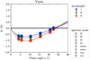 |
Fig. A.2 Same as Fig. A.1 but for Vesta. |
| In the text | |
Current usage metrics show cumulative count of Article Views (full-text article views including HTML views, PDF and ePub downloads, according to the available data) and Abstracts Views on Vision4Press platform.
Data correspond to usage on the plateform after 2015. The current usage metrics is available 48-96 hours after online publication and is updated daily on week days.
Initial download of the metrics may take a while.