| Issue |
A&A
Volume 684, April 2024
|
|
|---|---|---|
| Article Number | A118 | |
| Number of page(s) | 15 | |
| Section | Catalogs and data | |
| DOI | https://doi.org/10.1051/0004-6361/202348829 | |
| Published online | 10 April 2024 | |
A comprehensive search for hot subdwarf stars using Gaia and TESS
I. Pulsating hot subdwarf B stars★
1
Institute of Astronomy, KU Leuven,
Celestijnenlaan 200D,
3001
Leuven,
Belgium
e-mail: This email address is being protected from spambots. You need JavaScript enabled to view it.
2
Astronomical Observatory, Jagiellonian University,
ul. Orla 171,
30-244
Krakow,
Poland
3
Department of Physics, University of Warwick,
Gibbet Hill Road,
Coventry
CV4 7AL,
UK
4
Astronomical Institute of the Czech Academy of Sciences,
251 65,
Ondřejov,
Czech Republic
5
Astroserver.org,
Főtér 1,
8533
Malomsok,
Hungary
6
INAF-Osservatorio Astrofisico di Torino,
strada dell’Osservatorio 20,
10025
Pino Torinese,
Italy
7
Instituto de Física y Astronomía, Universidad de Valparaíso,
Gran Bretaña 1111,
Playa Ancha,
Valparaíso
2360102,
Chile
8
Institute for Physics and Astronomy, University of Potsdam,
Karl-Liebknecht-Str. 24/25,
14476
Potsdam,
Germany
Received:
3
December
2023
Accepted:
31
January
2024
Abstract
Hot subdwarf B (sdB) stars are evolved, subluminous, helium-burning stars that most likely form when red giant stars loose their hydrogen envelope via interactions with close companions. They play an important role in our understanding of binary evolution, stellar atmospheres, and interiors. Only a small fraction of the sdB population is known to exhibit pulsations. Pulsating sdBs have typically been discovered serendipitously in various photometric surveys because specific selection criteria for the sample are lacking. Consequently, while individual properties of these stars are well known, a comprehensive understanding of the entire population remains elusive, and many related questions remain unanswered. The Gaia mission has presented an exceptional chance to create an unbiased sample by employing precise criteria and ensuring a high degree of completeness. The progression of high-precision and high-duty cycle photometric monitoring facilitated by space missions such as Kepler/K2 and the Transiting Exoplanet Survey Satellite (TESS) has yielded an unparalleled wealth of data for pulsating sdBs. We created a dataset of confirmed pulsating sdB stars by combining information from various ground- and space-based photometric surveys. With this dataset, we present a thorough approach to search for pulsating sdB stars based on the current Gaia DR3 sample. Based on TESS photometry, we discovered 61 new pulsating sdB stars and 20 variable sdBs whose source of variability remains to be determined through future spectroscopic follow-up observations.
Key words: catalogs / stars: evolution / stars: horizontal-branch / stars: late-type / stars: oscillations / subdwarfs
Table A.3 is available at the CDS via anonymous ftp to cdsarc.cds.unistra.fr (130.79.128.5) or via https://cdsarc.cds.unistra.fr/viz-bin/cat/J/A+A/684/A118
© The Authors 2024
 Open Access article, published by EDP Sciences, under the terms of the Creative Commons Attribution License (https://creativecommons.org/licenses/by/4.0), which permits unrestricted use, distribution, and reproduction in any medium, provided the original work is properly cited.
This article is published in open access under the Subscribe to Open model. This email address is being protected from spambots. You need JavaScript enabled to view it. to support open access publication.
1 Introduction
Hot subdwarf B-type stars, referred to as sdB stars, are thought to be core-helium (He) burning stars characterized by an extremely thin hydrogen (H) envelope, with an envelope mass lower than 0.02 times the mass of the Sun, Meπv < 0.02 M⊙ (e.g., Ge et al. 2022). Their average mass is in close proximity to the mass at which the core-He flash occurs, approximately around 0.47 times the mass of the Sun (Fontaine et al. 2012). These sdB stars represent evolved compact objects with surface gravities (log 𝑔) in the range of 5.2–6.2 dex and effective temperatures (Teff) ranging from 20 000 to 40 000 K (Saffer et al. 1994; Green et al. 2008). They reside in the region between the main sequence and the cooling stage of white dwarfs, which is referred to as the region of extreme horizontal branch (EHB) stars (see Heber 2009, 2016, for a detailed overview). The evolutionary history of sdB stars involves significant mass loss, predominantly induced by binary interactions during the late stages of the red giant phase (Han et al. 2002, 2003). This phase results in the loss of almost the entire H-rich envelope, leaving behind a core that burns He, but the envelope is too thin to sustain H-shell burning. For approximately 108 yr, sdB stars continue to burn He in their cores. Following the depletion of He in their core, they transition into a phase in which He is burned in a shell surrounding a core composed of carbon and oxygen (C/O). They transform into subdwarf O (sdO) stars in this phase. Ultimately, these stars conclude their lifecycle as white dwarfs (e.g., Dorman et al. 1993).
Kilkenny et al. (1997) made the pioneering discovery of rapid pulsations in a subset of hot sdB stars. These stars have come to be known as V361 Hya stars and are often referred to as short-period sdB variable stars. The V361 Hya stars exhibit multiperiodic pulsations characterized by periods ranging from 60 s to 800 s. Within this frequency range, these pulsations correspond to low-degree, low-order pressure (p) modes. These modes are associated with photometric amplitudes that can reach up to several percent of the mean stellar brightness, as corroborated by studies conducted by Reed et al. (2007), Østensen et al. (2010), and Green et al. (2011). The excitation of these modes is attributed to a classical κ-mechanism, primarily driven by the accumulation of iron-group elements, with iron itself being a dominant contributor, in a region known as the Z-bump. This mechanism was elucidated by Charpinet et al. (1996) and further elaborated upon by Charpinet et al. (1997). These studies demonstrated that radiative levitation plays a crucial role as a physical process that enhances the concentrations of iron-group elements. This enhancement is a prerequisite for the activation of the pulsational modes. The p-mode sdB pulsators are typically located within a temperature range spanning from 28 000 K to 35 000 K, with surface gravities characterized by values in the range of log 𝑔 5–6 dex. Following this discovery, a different class of sdB pulsators known as V 1093 Her stars, exhibiting long-period pulsations, was identified by Green et al. (2003). These stars display variations in brightness with periods that can extend to a few hours and have amplitudes on the order of 0.1% or less of their mean brightness (e.g., Reed et al. 2011). The oscillation frequencies observed in these pulsators are linked to 𝑔-modes characterized by low-degree (l <3) and medium to high order (with 10 < n < 60), a phenomenon driven by the same κ-mechanism, caused by the accumulation of iron-group elements, as outlined by Fontaine et al. (2003) and further discussed by Charpinet et al. (2011). In contrast to the p-mode sdB pulsators, the 𝑔-mode sdB pulsators have somewhat cooler temperatures, ranging from 22 000 K to 30 000 K, and their surface gravities (log 𝑔) typically fall within the range of 5.0–5.5 dex. Within the spectrum of pulsating sdB stars, there exists a subset that is referred to as “hybrid” sdB pulsators, which exhibit both 𝑔- and p-modes concurrently (Schuh et al. 2006). These hybrid sdB pulsators occupy a distinct region in the Hertzsprung–Russell (HR) diagram that is positioned between the regions associated with p-mode and 𝑔-mode sdB pulsators, as depicted in Fig. 5 of Green et al. (2011). These objects hold particular significance as they provide a unique opportunity to conduct asteroseismic investigations, allowing for the study of both the core structure and the outer layers of sdBVs.
The Kepler (Borucki et al. 2010) and TESS missions (Ricker et al. 2014) both significantly contributed to identifying new candidate pulsating sdBs. During the primary Kepler mission, a group of 18 pulsating sdB stars was observed. Most of these stars, specifically, 16 of them, were identified as long-period 𝑔-mode pulsators, and the remaining 2 stars exhibited short-period p-mode pulsations (Østensen et al. 2010, 2011; Kawaler et al. 2010; Baran et al. 2011; Reed et al. 2011). Additionally, within the old open cluster NGC6791, three known sdB stars were also discovered to pulsate (Pablo et al. 2011; Reed et al. 2012). During the secondary Kepler mission, known as the K2 mission (Haas et al. 2014), about 50 sdBs were identified as pulsators, and ongoing analyses continue to study these stars. To date, papers about 20 of these sdBVs have been published, along with detailed information about their atmospheric parameters (Reed et al. 2016, 2019, 2020b; Ketzer et al. 2017; Bachulski et al. 2016; Baran et al. 2019; Silvotti et al. 2019; Østensen et al. 2020; Ma et al. 2022, 2023). The analysis of data from the TESS mission is currently ongoing, and a detailed analysis of 13 long-period sdBVs was reported (Charpinet et al. 2019; Reed et al. 2020a; Sahoo et al. 2020; Uzundag et al. 2021, 2023; Silvotti et al. 2022).
Holdsworth et al. (2017) compiled a table containing information on 110 known pulsating sdBs up to that point. In a subsequent review, Lynas-Gray (2021) provided a thorough overview, including 56 documented pulsating sdB stars. More recently, Van Grootel et al. (2021), Krzesinski & Balona (2022), and Baran et al. (2023) have made notable contributions by confirming and discovering new pulsating sdB stars, including short- and long-period sdBs, through observations conducted via the TESS mission.
In this study, an extensive dataset was meticulously assembled that encompasses all documented pulsating sdBV stars. This comprehensive compilation currently incorporates records for 256 pulsating sdBV stars. Based on this existing dataset, we developed a robust selection algorithm that we outline in Sect. 2. It is based on the Gaia color-magnitude diagram. In Sect. 3, we gather and analyze all accessible light curves from TESS, including both short- and ultrashort-cadence observations. Then, we generate periodograms for over 2300 objects. In Sect. 4, we classify the newly identified members. In Sects. 5 and 6, we present the spectroscopic observations and produce the atmospheric parameters of the newly discovered sdBs. We compare them with the established pulsating sdB population. Finally, we summarize our results and conclusions in Sect. 7.
2 Sample selection
Pulsating sdBs have mostly been found by chance in photometric campaigns, without clearly defined selection criteria for the sample. This means that while individual parameters can be very well determined, an understanding of the population as a whole is lacking, and many open questions remain, such as the pulsation occurrence rate. The advent of Gaia (Gaia Collaboration 2018) provided an unparalleled opportunity to assemble an unbiased sample by enabling the selection of candidates through well-defined criteria and a high level of completeness. Culpan et al. (2022) successfully compiled a catalog of 61 585 potential hot subdwarf candidates using Gaia EDR3 (Gaia Collaboration 2021).
In the pursuit of identifying potential pulsating sdB candidates, an initial step involved the comprehensive compilation of all known stars from the literature. This inclusive subset constituted 256 pulsating sdBs, which are visually represented by red dots in Fig. 1. We provide a catalog comprising all known pulsating sdBs in Table A.3. Subsequently, a distribution plot was constructed based on the known pulsating sdB stars, as shown in the right panel in Fig. 1. The mean value of the distribution is indicated by the horizontal dashed black line at MG = 4.18. Then, in order to encompass all known pulsating stars, we considered the ±σ range around the mean of the distribution. Therefore, the upper limit at +2σ is MG = 6.11, marked by the upper horizontal black line, while the lower limit at MG = 2.26, represented by the lower horizontal black line. To refine the selection, composite sdB systems such as sdBVs+F/G/K were excluded, specifically, those positioned beyond GBP − GRP > 0.1, as denoted by the vertical black line (future work will focus on the search for pulsating sdBs in binary systems). Following these refined criteria, an initial identification yielded a dataset of 25 615 stars. This dataset is shown in Fig. 1 with a blue shaded area.
In Fig. 1, we show the color–magnitude diagram of selected pulsating sdB candidates within the blue shaded area (left panel) along with known pulsating sdBs and their spatial distribution with respect to the Galactic coordinate system (right panel).
By limiting the sample to Gmag < 17 mag considering the TESS detection limit, we identified 10 452 targets. However, we note that setting a upper limit of Gmag < 17 can result in the exclusion of a few pulsators withlower amplitudes. To obtain all observed stars with TESS, we flanlly cross-matched the catalog with the TESS input catalog (Stassun et al. 2019), and the final sample was restricted to 2 371 objects with TESS light curves.
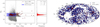 |
Fig. 1 Left: color–magnitude diagram of identified potential hot subdwarf candidates with gray dots from Culpan et al. (2022). We highlight 256 known sdBVs compiled from the literature in red. A distribution plot (middle panel) is constructed based on the known pulsating sdBs. The mean value of the distribution is indicated by the horizontal dashed black line, and the upper and lower limits are shown by horizontal black lines. Our refined sample, which excludes composite binaries, is visualized as a blue shaded box in the color–magnitude diagram. Right: sky locations (Galactic coordinates, Aitoff projection) of the selected pulsating sdB candidates that are observed with TESS and known pulsating sdBs with respect to the Galactic coordinate system using the same color-coding. |
3 TESS observations
TESS is actively observing numerous sdBs across the entire sky in consecutive sectors. Each sector is observed for a duration of approximately 27 days. The data from all the sectors (labeled from 1 to 68) covered by the TESS mission are currently accessible.
The TESS data are organized and stored in the Mikulski Archive for Space Telescopes (MAST)1 as target pixel files (TPFs) in FITS format. The light curves are accessible in two processed forms: calibrated using simple aperture photometry (SAP), and preconditioned through pre-search data conditioning simple aperture photometry (PDCSAP). For this work, we made use of PDCSAP, which was processed using the Science Processing Operations Center (SPOC) pipeline (Jenkins et al. 2016). The pipeline is based on the Kepler Mission science pipeline and is made available by the NASA Ames SPOC center and at the MAST archive.
The TESS light curves were obtained from MAST in two cadences: 2-minute (short cadence) light curves, available for all 2371 hot subdwarf candidates, and 20-s (ultrashort cadence) light curves, applicable to 808 out of the 2371 targets. Because of the extensive scope of this search for stellar variability, no specific effort was invested to optimize pipeline apertures.
Additionally, TPFs of interest were retrieved from the MAST archive, managed by the Lightkurve Collaboration (Lightkurve Collaboration 2018), for all candidates exhibiting variability. These TPFs comprise an 11 × 11 grid of pixels extracted from one of the four CCDs per camera where the target is located.
The TPFs were used to analyze fluxes in individual pixels of the pipeline apertures when the source of variability was uncertain. To gauge this uncertainty, we used the crowding factor, represented by the keyword CROWDSAP. This factor estimates the contamination level of the PDCSAP flux, providing the ratio of the target to the background star flux in the pipeline aperture, accounting for the presence of potentially bright sources near the target.
4 Variability search and classification method
In the following steps, we computed Lomb-Scargle periodograms (VanderPlas 2018) for each target light curve. The code that performed this task was based on the Python lightkurve package. To identify variability, a periodogram detection threshold of 5σ was applied. The frequency range to calculate the detection threshold extended from 0 to 360 day−1 for a 2-min cadence and 0 to 2160 day−1 for a 20-s cadence.
Variability in an object was evaluated by analyzing the maximum periodogram signal. If this signal surpassed the detection threshold, we proceeded to examine its frequency. In the initial step, we eliminated all stars displaying long-term variability and signals below the detection threshold, resulting in a subset of 1517 objects for the subsequent analysis.
It is important to note that sdBV pulsations are not expected at frequencies below 5 day−1. Any objects displaying maximum signals below 5 day−1 were therefore excluded from the sample. Additionally, objects exhibiting a strong signal (exceeding the periodogram detection threshold by a factor of 5) within the frequency range of 5–35 day−1 were systematically removed. This step aimed to eliminate potential binary systems from the sample. However, it is worth noting that compact binaries such as ZTF J213056.71+442046.5, with an orbital frequency of approximately 37 day−1 (Kupfer et al. 2020), could still be included in the sample of single pulsators. We identified two such objects: TIC107548305 and TIC 367090060, both exhibiting single peaks at frequencies of 40.833767 day−1 and 37.725309 day−1. In both cases, however, the presence of subharmonic frequencies in their periodograms, as well as the analysis of the phase-folded light curves, led us to conclude that the real period of these binaries is twice as long and corresponds to the subharmonic frequencies. Therefore, both stars were removed from our sample. While this procedure may inadvertently exclude some binaries featuring a pulsating primary sdB component, the primary focus remained on identifying single pulsators.
At this stage, our sample was refined to 284 objects whose periodograms met the criteria described above and underwent visual inspection. This inspection resulted in the removal of several clearly identified binary or eclipsing binary light curves, as well as objects with periodograms indicating subharmonics or harmonics to the main peaks. Consequently, our final sample comprises 61 objects that are classified as sdBV stars, as detailed in Table A.1, and 20 sdBs of uncertain type that are documented in Table A.2. The latter category encompasses stars displaying single peaks in their light-curve periodograms and an absence of subharmonics and harmonics. Some periodograms of these stars exhibit potential signals below the 5σ but above the 4-σ detection threshold. Due to the inherent difficulty in classification, most of these objects were labeled as binaries (B) or potential pulsating sdBs (G, I, P, or H, depending on the pulsation type, as outlined below).
The classification of pulsation types (indicated in the “Type” column of Tables A.1 and A.2) should be based on a theoretical division into 𝑔- and p-modes, determined by the pulsation periods of the stars. The theoretical works by Charpinet et al. (2000); Fontaine et al. (2003); Jeffery & Saio (2006); Hu et al. (2009); Bloemen et al. (2014) provided excitation region plots for 𝑔- and p-mode sdB pulsators in the period versus Teff space. While the period boundaries for 𝑔- and p-modes in these sources varied, the common range for mo-mode frequencies extends approximately from 4 to 55 day−1 (equivalent to periods 21600–1570 s, see Fig. 2 blue shaded region), and the p-mode excitation region can safely be assumed to lie above 340 day−1 (periods shorter than 250 s, as illustrated in Fig. 2 pink shaded region). For frequencies falling between these boundaries (Fig. 2 gray shaded region), it is challenging to classify a pulsation mode based solely on observed frequencies in the Lomb-Scargle periodograms from photometric data alone.
To visualize the problem of a classification that relies on photometric measurements, we conducted an analysis to determine the positions of pulsation frequencies within the amplitude diagram. This involved collecting periodicities from stars observed during the Kepler and K2 missions, excluding sdBVs found in binary systems. The dataset comprised 18 rich2 pulsating sdBs3, totaling 1630 individual frequencies identified in previous works. In Fig. 2, we illustrate the frequency distribution of this dataset. As depicted, frequencies between ~4 to 55 day−1, corresponding to 𝑔-modes, constitute the most prevalent group of modes excited in sdBV stars. However, 𝑔-mode frequencies in Kepler sdBVs were found up to 86 day−1, while p-modes begin to show above 172 day−1. Frequencies between these two boundaries are considered intermediate modes.
As demonstrated, the theoretical division based on the common frequency ranges in all the mentioned theoretical works does not align precisely with the observed frequencies (e.g., the group of modes between 55–86 day−1, which might be a continuation of 𝑔-modes, or the group of modes above 172 day−1, which might belong to p-modes). This suggests that relying on photometry alone, we cannot provide accurate classification when a mode falls within the theoretical transition region.
To avoid confusion, we chose here to adhere to the classification that is based on the regions where theoretical works converge. We defer a precise mode identification to future investigations. Therefore, in Tables A.1 and A.2, we classify stars as 𝑔-mode pulsators when the observed frequencies were between 5 and 55 day−1 (labeled ‘G’ in the “Type” column), as p-modes (‘P’) when a periodogram frequency was above 340 day−1, and as intermediate mode pulsators when the observed frequencies fell between 55 and 340 day−1. To classify a star as a hybrid-mode pulsator (‘H’), it would need to meet both the G and P classification criteria. Furthermore, in Col. 8 (frequencies [day−1 ], peaks; see Table A.1), we provide the observed signal frequency ranges (in day−1) and the corresponding number of signal peaks. Similarly, in Table A.2, Col. 8 includes the frequencies of single peaks, along with details on subharmonics or harmonics and any additional frequencies present in the periodograms.
Periodograms for all new variable sdBs from both Tables A.1 and A.2 are presented in Fig. A.1 for the 61 sdBVs and in Fig. A.2 for the 20 sdBs of uncertain variability. Notably, Tables A.1 and A.2 reveal that some objects exhibit a low CROWDSAP factor, suggesting possible flux contamination from background stars. Consequently, all objects with a CROWDSAP factor below 0.6 underwent additional scrutiny employing TPFs to assess the target variability. We did not attempt to recover the actual pulsation amplitudes, which are diminished due to the light pollution from the nearby stars that affects the targets.
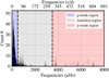 |
Fig. 2 Frequency distribution of pulsating sdBs that were observed by Kepler/K2. The theoretical boundaries for 𝑔- and p-mode regions are represented by the vertical dashed black lines. See text for more details. |
5 Spectroscopic observations
The follow-up spectroscopic observations of the sdB pulsators analyzed in this study were conducted using three distinct instruments. These instruments are the Boller and Chivens (B&C) spectrograph installed on the 2.5-m (100-inch) Irénée du Pont Telescope4 at Las Campanas Observatory in Chile, the European Southern Observatory (ESO) Faint Object Spectrograph and Camera (v.2) (EFOSC2; Buzzoni et al. 1984) mounted at the Nasmyth B focus of the New Technology Telescope (NTT) at La Silla Observatory in Chile, and the Southern Astrophysical Research (SOAR) Telescope, a 4.1-m aperture optical and near-infrared telescope (Clemens et al. 2004), located at Cerro Pachón, Chile.
We acquired low-resolution spectra to determine the atmospheric parameters, including the effective temperature (Teff), surface gravity (log g), and helium (He) abundance. Two sdB stars, TIC152373379 and TIC394678374, were observed with the B&C spectrograph, while three sdBs, TIC269766236, TIC332841294, and TIC340223812, were observed with the EFOSC2. Only one sdB star, TIC181914779, was observed with the Goodman spectrograph.
The B&C spectra were obtained using the 600 lines/mm grating, corresponding to a central wavelength of 5000 Å, and covering a wavelength range from 3427 to 6573 Å. A 1 arcsec slit was used, resulting in a resolution of 3.1 Å. In the case of EFOSC2 setup, the 6.4 Å resolution was obtained with a setup of grism 7 and a 1 arcsec slit. In the case of the Goodman spectrograph, the 400 mm−1 grating with the blaze wavelength 5500 Å (M1: 3000–7050 Å) with a slit of 1 arcsec was used and this setup provides a resolution of about 5.6 Å.
The data from B&C and EFOSC2 were reduced and analysed using PyRAF5 (Science Software Branch at STScI 2012) procedures in the following way: First, bias correction and flat-field correction were applied. Then, the pixel-to-pixel sensitivity variations were removed by dividing each pixel by the response function. After this reduction was completed, we applied wavelength calibrations using the frames obtained with the internal He–Ar comparison lamp. In a last step, flux calibrations were applied using the standard stars. The data reduction for Goodman was partially made by using the instrument pipeline6, including overscan, trim, slit trim, bias, and flat corrections. To identify and remove cosmic rays, we used the algorithm described by Pych (2004), which is embedded in the pipeline. The extraction and calibration of the spectra was carried out similarly as for B&C and EFOSC2 using standard PyRAF tasks. The details of the spectroscopic observations are given in Table 1 including the instrument, date, exposure time, and resolution.
Observing log of the spectroscopic data obtained for six pulsating sdB stars.
6 Spectroscopic parameters
We employed a steepest-descent procedure implemented in XTGRID (Németh et al. 2012), which is specifically designed for automating the spectral analysis of early-type stars using TLUSTY/SYNSPEC (Hubeny & Lanz 2017) nonlocal thermody-namic equilibrium (non-LTE) stellar atmosphere models. This method employs an iterative chi-square minimization approach to fit observed data. Commencing with an initial model, the process converges on the best fit through successive approximations along the chi-square gradient. To reduce systematic effects such as blaze function correction, flexure, or flux inconsistencies due to vignetting or slit-loss, the models were compared with observations via a piecewise normalization.
To determine the parameters of hot stars, both the completeness of included opacity sources and departures from LTE are crucial for accuracy. We determined that TLUSTY models, characterized by H, He composition, yield reliable results within the constraints of spectral resolution, coverage, and signal-to-noise ratio of the survey data.
XTGRID dynamically computes the required TLUSTY atmosphere models and synthetic spectra, incorporating a recovery method to tolerate convergence failures and expedite convergence on a solution with a minimum number of models. Figure 3 shows the best fits for the spectra of the six newly discovered variable sdB stars. The surface parameters are listed at the top of Table2.
Parameter errors are assessed by mapping the chi-square statistics around the solution. The parameters were altered in one dimension until the 60% confidence limit was reached. Correlations near the best-fit values were incorporated into the final results for the surface temperature and gravity.
We compiled a catalog comprising 256 known pulsating hot subdwarf stars. The stars are listed in Table A.3. Within the literature, atmospheric parameters are available for 149 out of the total 256 stars included in our catalog. In addition, in Table 2, we present the atmospheric parameters and Gaia distances for 22 of 61 newly discovered pulsating sdB stars presented in Table A.1. The stars listed in Table 2 are arranged in order of their effective temperatures. The initial five stars listed in the table are those identified in the current investigation by spectroscopic observations, and the parameters for the remaining stars from Table 2 were inferred from the literature. The remaining 39 stars that are listed in Table A.1 require additional spectroscopic observations. Our efforts are continuing, and in future work, we will present their atmospheric parameters. Figure 4 illustrates the newly found pulsating sdBs marked with red squares, while previously known ones are represented by blue dots.
Table 3 reports the atmospheric parameters for an additional 9 of the 20 new variable sdB stars listed in Table A.2 whose variability we classified as uncertain. The first star, TIC 394678374 in Table 3, was identified in this work by spectroscopic observations. The parameters for the remaining stars from Table 3 were obtained from the literature. The location of most of them within the instability strip as depicted by the open red squares in Fig. 4 suggests that they are potential pulsators. However, the amplitude spectra in Fig. A.4 show either a single peak or a few peaks, which could originate from binarity or pulsation. Notably, TIC 125556577, positioned outside the 𝑔- and p-mode instability regions, may be a novel pulsating hot subdwarf O star. To confirm the nature of the variability, future photometric measurements for all targets in Table 3 are needed.
The evolutionary tracks from Uzundag et al. (2021), based on stellar evolution models using the LPCODE code (Althaus et al. 2005; Miller Bertolami 2016), are plotted in Fig. 4. These tracks, indicated by thick black lines, cover a mass range from Mzahb = 0.46738 to 0.473 M⊙, with ℓ = 1 the 𝑔-mode frequencies computed using the adiabatic nonradial pulsation code LP – PUL (Córsico & Althaus 2006).
In Fig. 5, the distribution of all pulsating sdBs (179 stars) is depicted in the effective temperature, log 𝑔, and log(y) plane. As anticipated, the Teff distribution (first panel) shows a bimodal pattern, segregating stars into 𝑔- and p-modes. The range of Teff between 20 000 K and 28 000 K encompasses most 𝑔-mode dominated sdBs, while the higher Teff range from 32 000 K to 40 000 K includes p-mode dominated stars. Hybrid stars are situated in these two regions, with hybridity observed across the entire span from 20 000 K to 40 000 K. The log 𝑔 distribution exhibits a relatively narrow spread, with the majority of pulsating sdBs concentrated between 5 and 6. The distribution peaks at 5.55, indicating a central tendency within this log 𝑔 range.
In Fig. 6, we used the Teff versus log(y) diagram, employing the classification scheme from Németh et al. (2012) and later refined by Luo et al. (2019), to distinguish the He abundance in pulsating sdB stars. The sdB parameter space is split into He-rich (shaded light blue region) and He-deficient (shaded green area) stars. These divisions are then further classified into He-poor (pHe), He-weak (wHe), and intermediate He-rich (iHe) classes. The majority of pulsating sdB stars belong to the pHe class. The two groups including 𝑔- and p-mode pulsating sdBs separate very well in both Teff versus log 𝑔 and He abundance. P-mode pulsators are frequent among the hotter pHe stars, while the 𝑔- mode is dominant among wHe stars. Moreover, the number of pulsating sdBs drops significantly in the He-rich range.
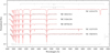 |
Fig. 3 Best-fit TLUSTY/XTGRID models (red) for the collection of continuum-normalized spectra (gray) of the newly discovered variable sdB stars, organized by increasing Teff from the bottom. For a better representation the identified in the current investigation by spectroscopic observations, while parameters for the remaining stars from Tables 2 and 3 were inferred from the literature. The observed fluxes were adjusted to the final models, and the adjacent spectra were shifted by 25%. |
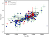 |
Fig. 4 Position of the spectroscopically identified pulsating sdB star indicated in the Teff–log 𝑔 plane. The known pulsating sdBs are represented by blue dots, and the newly discovered pulsating sdBs are denoted by red squares from Table A.1. The open red squares present promising pulsating sdB candidates from Table A.2. The evolutionary tracks have been adapted from Uzundag et al. (2021). |
7 Summary, discussion, and future prospects
We generated a dataset comprising confirmed pulsating sdB stars by consolidating data from different ground- and space-based photometric surveys. Employing this dataset, we conducted a comprehensive investigation to identify pulsating sdB stars within the existing Gaia DR3 sample. Through the analysis of TESS photometry for 2371 stars, we discovered 81 new variable sdB stars, comprising 61 pulsating stars (refer to Table A.1) and 20 sdBs exhibiting uncertain variability (refer to Table A.2). The specific nature of the variability in these 20 stars requires additional investigation, which will be carried out through subsequent spectroscopic and photometric follow-up observations.
We determined the atmospheric parameters for six stars by matching synthetic spectra to the recently acquired low-resolution spectra from Dupont/B&C, NTT/EFOSC2, and SOAR/Goodman. Additionally, we collected the atmospheric parameters from the literature for 17 stars. The newly discovered sdB pulsating stars have effective temperatures ranging from 24 220 K to 33 841 K, and their surface gravity (log 𝑔) falls within the range of 5.1–5.8 dex. This confirms that these stars distinctly belong to the 𝑔- and p-mode sdBV parameter space.
Concerning our mode classification presented in Tables A.1, A.2, the classification of pulsation modes based on Kepler sdBVs shown in Fig. 2 would lead to the inference that gravity modes typically extend up to 86 day−1, intermediate modes are situated between 86 and 172 day−1, and acoustic p-modes are above 172 day−1. This would change our mode classification in both Tables A.1 and A.2. However, the classification derived from the frequency position in Fig. 2 is based on its occurrence according to a set of the best-investigated sdBV periodograms and constitutes rather an experimental or statistical approach, while more theoretical work in this regard is necessary.
Additionally, the objects presented in Table A.2 (Fig. A.4) exhibit single frequencies (in some cases, two frequencies) located in the low-frequency regions, that is, below 40 day−1. This frequency region also corresponds to the binary orbital frequency range; but in the absence of indications of subharmonic or harmonic frequencies and phased light curves not showing any clear evidence of binarity, a differentiation between binary and pulsating 𝑔-modes is impossible based on photometric observations alone. Therefore, future spectroscopic observations of these objects are necessary to classify these stars better. Ongoing and future large scale spectroscopic surveys such as The Large Sky Area Multi-Object Fiber Spectroscopic Telescope (LAMOST; Cui et al. 2012), the Sloan Digital Sky Survey V (SDSS-V; Kollmeier et al. 2017), WEAVE (Jin et al. 2023), and 4MOST (de Jong et al. 2019) will be quite important to confirm the spectroscopic types of hot subdwarfs and to increase the size of the sample. Furthermore, future photometric observations from space, such as TESS and the PLAnetary Transits and Oscillations mission (PLATO, Rauer et al. 2014; Piotto 2018), or from ground-based initiatives such as the Large Synoptic Survey Telescope (LSST; Ivezic et al. 2019) or BlackGEM (Bloemen et al. 2015), will contribute insights into the nature of the variabilities for the stars that are presented in this work.
These surveys will allow us to create a volume-limited sample of sdBs. The initial efforts were undertaken to create the first volume-limited sample of hot subdwarfs covering a range up to 500 pc (Dawson et al. 2024). Our forthcoming research will specifically concentrate on characterizing pulsating sdBs within 500 pc to determine the pulsation occurrence rate. Furthermore, these surveys will allow us to characterize the stars for which spectroscopic measurements are currently unavailable, as presented in Table A.3. Every star featured in this study holds significant value as input for modeling purposes. Including the findings presented here, pulsational variability of 317 pulsating sdBs has been documented to date. However, only a small fraction of these stars has undergone an in-depth asteroseismic analysis. The identification of common patterns in the pulsation spectrum in pulsating sdBs will guide our comparison of the measured frequencies to stellar models. Therefore, developing a dedicated pipeline for a detailed seismic analysis for all pulsating sdBs presented in this work is crucial.
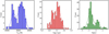 |
Fig. 5 Distribution plots displaying Teff (first panel), log 𝑔 (second panel), and log(y) (third panel) for 179 pulsating sdBs for which atmospheric parameters are known. |
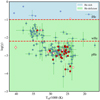 |
Fig. 6 Teff vs. log(y) diagram using the classification scheme from Németh et al. (2012) to discern the helium (He) abundance in pulsating sdB stars. The parameter space for sdBs is divided into He-rich (shaded light blue region) and He-deficient (shaded green area) stars. These divisions are subsequently categorized into He-poor (pHe), He-weak (wHe), and intermediate He-rich (iHe) classes. The color-codes for the targets are the same as in Fig. 4. |
Acknowledgements
M.U. gratefully acknowledges funding from the Research Foundation Flanders (FWO) by means of a junior postdoctoral fellowship (grant agreement no. 1247624N). I.P. acknowledges support a Royal Society University Research Fellowship (URF\R1\231496). H.D. is supported by the Deutsche Forschungsgemeinschaft (DFG) through grant GE2506/17-1. P.N. acknowledges support from the Grant Agency of the Czech Republic (GAČR 22-34467S). The Astronomical Institute in Ondřejov is supported by the project RVO:67985815. This research has used the services of www.Astroserver.org under reference W2MSWR. The research has made use of TOPCAT, an interactive graphical viewer and editor for tabular data Taylor (Taylor 2005). This research made use of the SIMBAD database, operated at CDS, Strasbourg, France; the VizieR catalogue access tool, CDS, Strasbourg, France. This work has made use of data from the European Space Agency (ESA) mission Gaia (https://www.cosmos.esa.int/gaia), processed by the Gaia Data Processing and Analysis Consortium (DPAC, https://www.cosmos.esa.int/web/gaia/dpac/consortium).
Appendix A Tables and figures
Appendix A.1 Notes on objects in Table A.1 and A.2
Fourteen stars in A.1 were identified as intermediate (or GI) mode pulsators. All except for three objects pulsate at intermediate frequencies higher than 160 d−1. The three exceptions are listed below.
TIC 3905338: This object is recognized as a 𝑔-mode pulsator with consecutive frequencies extending from 47 up to 60 d−1. Therefore, a few frequencies fall above the 55 d−1 frequency limit considered in this paper as a common maximum frequency for 𝑔-mode pulsators (i.e., in agreement with all theoretical works). Interestingly, the light-curve periodogram of this star shows a quite regular series of frequencies separated by 0.42 d−1, which might be a result of frequency splittings of a few pulsation modes.
TIC 241065253: This 𝑔-mode pulsator also exhibits two frequencies in the range between 85-95 d−1. There is a clear ~250-second period spacing between roughly seven 𝑔-modes, indicating l1-mode excitation. Additionally, the light-curve periodogram shows a signal at 0.714 d−1, which might be assigned to an orbital frequency. However, this cannot be confirmed via visual inspection because the amplitude of the assumed orbital signal is low (most pulsating modes have higher amplitudes).
TIC 325253096: The periodogram of this object only shows a single frequency at 76.8 d−1.
Other interesting objects from Table A.1 are listed below.
TIC 222892604: Only two peaks are visible in the intermediate-frequency range of the light-curve periodogram. A frequency at 290.7124 d−1 has an amplitude exceeding the detection threshold by more than 15 times, and it also shows an indication of splitting into a triplet.
TIC 269766236: The periodogram for this star shows clear period spacing of ~250 seconds between nine modes, indicating l1 -mode excitation.
TIC 313007038: This object is identified as a GI mode pulsator. Its periodogram shows three 𝑔-mode signals with a low amplitude between 9-25 d−1 and three frequencies between 230 - 250 d−1. The frequency at 248.36997 d−1 has an amplitude that exceeds the detection threshold by almost ten times.
TIC 441725813: This star has rich and high-amplitude pulsation modes (compared to the detection threshold). The data for this star cover over 570 days across 14 seasons. There is an evident period spacing of approximately 260-270 seconds. The pulsation modes extend up to 390 d−1 (visible in the ultrashort-cadence data periodogram); we therefore identified the star as a hybrid pulsator.
At the end of Table A.1, we present six p-mode pulsators found using ultrashort-cadence data. Five of them exhibit a few (two to four) pulsation frequencies in proximity to 600 d−1; however, TIC 99499703 only shows a single frequency at 972.7577 d−1.
There is only a handful of objects in Table A.2 that might be more interesting than the others.
TIC 183799565: The light-curve periodogram for this star only shows a single frequency at 34.793 d−1. If this were considered as the orbital frequency, it would correspond to one of the shortest orbital periods observed for sdB binaries. However, due to the low amplitude of this signal, a visual inspection of the phase-folded light curve reveals a large scatter, making it challenging to discern the shape of a possible binary light curve.
TIC 165453703, TIC 239122172, TIC 241514378, and TIC 443554222: They display an indication of asymmetrical phase-folded light curves and single frequencies in their periodograms. These stars are more likely to be pulsators than binaries.
As mentioned in Section 3, stars with a low CROWDSAP factor (below 0.6) were examined to determine whether they caused the observed variability in the periodograms, as opposed to neighboring stars. However, in several cases, discerning the variability of a target or a neighboring star within the same pixel was challenging based on TPF file pixels alone. In these instances, we relied on the patterns of frequencies, referred to as an sdBV pulsation pattern (primarily feasible only for objects from Table A.1), visible in periodograms and the positions of neighboring stars from the TESS pipeline apertures in the HR diagram.
We used HR diagrams based on Gaia data. In most cases, neighboring stars were situated in the main-sequence regions where sdBV pulsations cannot be observed. We therefore considered these variable targets as properly identified.
In Table A.2, 4 out of 20 objects exhibit a low-CROWDSAP factor, namely TIC 95960421, TIC 239122172, TIC 270285517, and TIC 443554222. Their periodograms reveal only single frequencies with low amplitudes. As a result, we were unable to confirm the variability of these stars. Further verification using ground-based and higher-resolution telescopes is necessary.
Sixty-one new sdBVs are presented, including columns for TIC number, right ascension, declination, TESS magnitude, crowdedness factor (CROWDSAP), number of TESS runs, pulsation type (G - gravity mode, I - intermediate mode, P - acoustic mode, H - hybrid mode), and notes.
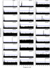 |
Fig. A.1 Lomb-Scargle periodograms of the 61 newly found sdBV stars (27 objects from table A.1 are shown). The horizontal blue lines are 5 σ detection thresholds. |
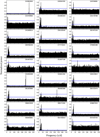 |
Fig. A.2 Continuation of Fig. A.1: Lomb-Scargle periodograms of the next 27 sdBV stars from table A.1. The horizontal blue lines are 5 σ detection thresholds. |
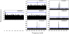 |
Fig. A.3 Continuation of Fig. A.1: Lomb-Scargle periodograms of the last sdBV (lef side) from the top part of table A.1 and six p-mode pulsators found in the ultrashort cadence (20 sec integration time) data. The horizontal blue lines are 5 σ detection thresholds. |
Twenty sdB stars of uncertain variability type are presented, including columns for TIC number, right ascension, declination, TESS magnitude, CROWDSAP, number of TESS runs, variability type (B - binary, R - rotation, G - gravity mode), and notes.
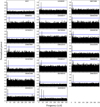 |
Fig. A.4 Periodograms of 20 sdB stars from table A.2 of uncertain variability. The horizontal blue lines are 5 σ detection thresholds. |
References
- Althaus, L. G., Serenelli, A. M., Panei, J. A., et al. 2005, A&A, 435, 631 [NASA ADS] [CrossRef] [EDP Sciences] [Google Scholar]
- Bachulski, S., Baran, A. S., Jeffery, C. S., et al. 2016, Acta Astron., 66, 455 [Google Scholar]
- Baran, A. S., Kawaler, S. D., Reed, M. D., et al. 2011, MNRAS, 414, 2871 [NASA ADS] [CrossRef] [Google Scholar]
- Baran, A. S., Telting, J. H., Jeffery, C. S., et al. 2019, MNRAS, 489, 1556 [Google Scholar]
- Baran, A. S., Van Grootel, V., Østensen, R. H., et al. 2023, A&A, 669, A48 [NASA ADS] [CrossRef] [EDP Sciences] [Google Scholar]
- Bloemen, S., Hu, H., Aerts, C., et al. 2014, A&A, 569, A123 [NASA ADS] [CrossRef] [EDP Sciences] [Google Scholar]
- Bloemen, S., Groot, P., Nelemans, G., & Klein-Wolt, M. 2015, Living Together: Planets, Host Stars and Binaries, eds. S. M. Rucinski, G. Torres, & M. Zejda, ASP Conf. Ser., 496, 254 [NASA ADS] [Google Scholar]
- Borucki, W. J., Koch, D., Basri, G., et al. 2010, Science, 327, 977 [Google Scholar]
- Buzzoni, B., Delabre, B., Dekker, H., et al. 1984, The Messenger, 38, 9 [NASA ADS] [Google Scholar]
- Charpinet, S., Fontaine, G., Brassard, P., & Dorman, B. 1996, ApJ, 471, L103 [Google Scholar]
- Charpinet, S., Fontaine, G., Brassard, P., et al. 1997, ApJ, 483, L123 [Google Scholar]
- Charpinet, S., Fontaine, G., Brassard, P., & Dorman, B. 2000, ApJS, 131, 223 [Google Scholar]
- Charpinet, S., Van Grootel, V., Fontaine, G., et al. 2011, A&A, 530, A3 [NASA ADS] [CrossRef] [EDP Sciences] [Google Scholar]
- Charpinet, S., Brassard, P., Fontaine, G., et al. 2019, A&A, 632, A90 [NASA ADS] [CrossRef] [EDP Sciences] [Google Scholar]
- Clemens, J. C., Crain, J. A., & Anderson, R. 2004, SPIE Conf. Ser., 5492, 331 [NASA ADS] [Google Scholar]
- Córsico, A. H., & Althaus, L. G. 2006, A&A, 454, 863 [NASA ADS] [CrossRef] [EDP Sciences] [Google Scholar]
- Cui, X.-Q., Zhao, Y.-H., Chu, Y.-Q., et al. 2012, Res. Astron. Astrophys., 12, 1197 [Google Scholar]
- Culpan, R., Geier, S., Reindl, N., et al. 2022, A&A, 662, A40 [NASA ADS] [CrossRef] [EDP Sciences] [Google Scholar]
- Dawson, H., Geier, S., Heber, U., et al. 2024, A&A, in press, https://doi.org/10.1051/0004-6361/202348319 [Google Scholar]
- de Jong, R. S., Agertz, O., Berbel, A. A., et al. 2019, The Messenger, 175, 3 [NASA ADS] [Google Scholar]
- Dorman, B., Rood, R. T., & O’Connell, R. W. 1993, ApJ, 419, 596 [NASA ADS] [CrossRef] [Google Scholar]
- Edelmann, H., Heber, U., Hagen, H. J., et al. 2003, A&A, 400, 939 [NASA ADS] [CrossRef] [EDP Sciences] [Google Scholar]
- Fontaine, G., Brassard, P., Charpinet, S., et al. 2003, ApJ, 597, 518 [Google Scholar]
- Fontaine, G., Brassard, P., Charpinet, S., et al. 2012, A&A, 539, A12 [NASA ADS] [CrossRef] [EDP Sciences] [Google Scholar]
- Gaia Collaboration (Brown, A. G. A., et al.) 2018, A&A, 616, A1 [NASA ADS] [CrossRef] [EDP Sciences] [Google Scholar]
- Gaia Collaboration (Brown, A. G. A., et al.) 2021, A&A, 649, A1 [NASA ADS] [CrossRef] [EDP Sciences] [Google Scholar]
- Ge, H., Tout, C. A., Chen, X., et al. 2022, ApJ, 933, 137 [NASA ADS] [CrossRef] [Google Scholar]
- Geier, S., Heber, U., Podsiadlowski, P., et al. 2010, A&A, 519, A25 [NASA ADS] [CrossRef] [EDP Sciences] [Google Scholar]
- Geier, S., Østensen, R. H., Nemeth, P., et al. 2017, Open Astron., 26, 164 [NASA ADS] [CrossRef] [Google Scholar]
- Green, E. M., Fontaine, G., Reed, M. D., et al. 2003, ApJ, 583, L31 [Google Scholar]
- Green, E. M., Fontaine, G., Hyde, E. A., For, B. Q., & Chayer, P. 2008, Hot Subdwarf Stars and Related Objects, eds. U. Heber, C. S. Jeffery, & R. Napiwotzki, ASP Conf. Ser., 392, 75 [NASA ADS] [Google Scholar]
- Green, E. M., Guvenen, B., O’Malley, C. J., et al. 2011, ApJ, 734, 59 [Google Scholar]
- Haas, M. R., Barclay, T., Batalha, N. M., et al. 2014, in Am. Astron. Soc. Meeting Abstracts, #223, 228.01 [Google Scholar]
- Han, Z., Podsiadlowski, P., Maxted, P. F. L., Marsh, T. R., & Ivanova, N. 2002, MNRAS, 336, 449 [Google Scholar]
- Han, Z., Podsiadlowski, P., Maxted, P. F. L., & Marsh, T. R. 2003, MNRAS, 341, 669 [NASA ADS] [CrossRef] [Google Scholar]
- Heber, U. 2009, ARA&A, 47, 211 [Google Scholar]
- Heber, U. 2016, PASP, 128, 082001 [Google Scholar]
- Holdsworth, D. L., Østensen, R. H., Smalley, B., & Telting, J. H. 2017, MNRAS, 466, 5020 [Google Scholar]
- Hu, H., Nelemans, G., Aerts, C., & Dupret, M. A. 2009, A&A, 508, 869 [NASA ADS] [CrossRef] [EDP Sciences] [Google Scholar]
- Hubeny, I., & Lanz, T. 2017, arXiv e-prints [arXiv: 1706.01859] [Google Scholar]
- Hunger, K., Gruschinske, J., Kudritzki, R. P., & Simon, K. P. 1981, A&A, 95, 244 [NASA ADS] [Google Scholar]
- Ivezic, Ž., Kahn, S. M., Tyson, J. A., et al. 2019, ApJ, 873, 111 [NASA ADS] [CrossRef] [Google Scholar]
- Jeffery, C. S., & Saio, H. 2006, MNRAS, 372, L48 [NASA ADS] [CrossRef] [Google Scholar]
- Jenkins, J. M., Twicken, J. D., McCauliff, S., et al. 2016, Proc. SPIE, 9913, 99133E [Google Scholar]
- Jin, S., Trager, S. C., Dalton, G. B., et al. 2023, MNRAS, in press, https://doi.org/10.1093/mnras/stad557 [Google Scholar]
- Kawaler, S. D., Reed, M. D., Quint, A. C., et al. 2010, MNRAS, 409, 1487 [Google Scholar]
- Ketzer, L., Reed, M. D., Baran, A. S., et al. 2017, MNRAS, 467, 461 [NASA ADS] [Google Scholar]
- Kilkenny, D., Koen, C., O’Donoghue, D., & Stobie, R. S. 1997, MNRAS, 285, 640 [Google Scholar]
- Kollmeier, J. A., Zasowski, G., Rix, H.-W., et al. 2017, arXiv e-prints [arXiv:1711.03234] [Google Scholar]
- Krzesinski, J., & Balona, L. A. 2022, A&A, 663, A45 [NASA ADS] [CrossRef] [EDP Sciences] [Google Scholar]
- Kupfer, T., Geier, S., Heber, U., et al. 2015, A&A, 576, A44 [NASA ADS] [CrossRef] [EDP Sciences] [Google Scholar]
- Kupfer, T., Bauer, E. B., Marsh, T. R., et al. 2020, ApJ, 891, 45 [Google Scholar]
- Lightkurve Collaboration (Cardoso, J. V. d. M., et al.) 2018, Astrophysics Source Code Library [record ascl:1812.813] [Google Scholar]
- Lisker, T., Heber, U., Napiwotzki, R., et al. 2005, A&A, 430, 223 [NASA ADS] [CrossRef] [EDP Sciences] [Google Scholar]
- Luo, Y., Németh, P., Deng, L., & Han, Z. 2019, ApJ, 881, 7 [NASA ADS] [CrossRef] [Google Scholar]
- Luo, Y., Németh, P., Wang, K., Wang, X., & Han, Z. 2021, ApJS, 256, 28 [NASA ADS] [CrossRef] [Google Scholar]
- Lynas-Gray, A. E. 2021, Front. Astron. Space Sci., 8, 19 [NASA ADS] [Google Scholar]
- Ma, X.-Y., Zong, W., Fu, J.-N., et al. 2022, ApJ, 933, 211 [CrossRef] [Google Scholar]
- Ma, X.-Y., Zong, W., Fu, J.-N., et al. 2023, A&A, 680, A11 [NASA ADS] [CrossRef] [EDP Sciences] [Google Scholar]
- Miller Bertolami, M. M. 2016, A&A, 588, A25 [NASA ADS] [CrossRef] [EDP Sciences] [Google Scholar]
- Németh, P., Kawka, A., & Vennes, S. 2012, MNRAS, 427, 2180 [Google Scholar]
- Østensen, R. H., Silvotti, R., Charpinet, S., et al. 2010, MNRAS, 409, 1470 [CrossRef] [Google Scholar]
- Østensen, R. H., Silvotti, R., Charpinet, S., et al. 2011, MNRAS, 414, 2860 [CrossRef] [Google Scholar]
- Østensen, R. H., Jeffery, C. S., Saio, H., et al. 2020, MNRAS, 499, 3738 [Google Scholar]
- Pablo, H., Kawaler, S. D., & Green, E. M. 2011, ApJ, 740, L47 [NASA ADS] [CrossRef] [Google Scholar]
- Piotto, G. 2018, in European Planetary Science Congress, EPSC2018-969 [Google Scholar]
- Pych, W. 2004, PASP, 116, 148 [NASA ADS] [CrossRef] [Google Scholar]
- Rauer, H., Catala, C., Aerts, C., et al. 2014, Exp. Astron., 38, 249 [Google Scholar]
- Reed, M. D., Terndrup, D. M., Eggen, J. R., & Unterborn, C. T. 2007, Commun. Asteroseismol., 150, 269 [Google Scholar]
- Reed, M. D., Baran, A., Quint, A. C., et al. 2011, MNRAS, 414, 2885 [Google Scholar]
- Reed, M. D., Baran, A., Østensen, R. H., Telting, J., & O’Toole, S. J. 2012, MNRAS, 427, 1245 [Google Scholar]
- Reed, M. D., Baran, A. S., Østensen, R. H., et al. 2016, MNRAS, 458, 1417 [Google Scholar]
- Reed, M. D., Telting, J. H., Ketzer, L., et al. 2019, MNRAS, 483, 2282 [NASA ADS] [Google Scholar]
- Reed, M. D., Shoaf, K. A., Németh, P., et al. 2020a, MNRAS, 493, 5162 [Google Scholar]
- Reed, M. D., Yeager, M., Vos, J., et al. 2020b, MNRAS, 492, 5202 [Google Scholar]
- Ricker, G. R., Winn, J. N., Vanderspek, R., et al. 2014, SPIE Conf. Ser., 9143, 914320 [Google Scholar]
- Saffer, R. A., Bergeron, P., Koester, D., & Liebert, J. 1994, ApJ, 432, 351 [NASA ADS] [CrossRef] [Google Scholar]
- Sahoo, S. K., Baran, A. S., Heber, U., et al. 2020, MNRAS, 495, 2844 [Google Scholar]
- Schuh, S., Huber, J., Dreizler, S., et al. 2006, A&A, 445, L31 [NASA ADS] [CrossRef] [EDP Sciences] [Google Scholar]
- Science Software Branch at STScI 2012, Astrophysics Source Code Library [record ascl:1207.011] [Google Scholar]
- Silvotti, R., Uzundag, M., Baran, A. S., et al. 2019, MNRAS, 489, 4791 [Google Scholar]
- Silvotti, R., Németh, P., Telting, J. H., etal. 2022, MNRAS, 511, 2201 [NASA ADS] [CrossRef] [Google Scholar]
- Stassun, K. G., Oelkers, R. J., Paegert, M., et al. 2019, AJ, 158, 138 [Google Scholar]
- Taylor, M. B. 2005, Astronomical Data Analysis Software and Systems XIV, eds. P. Shopbell, M. Britton, & R. Ebert, ASP Conf. Ser., 347, 29 [NASA ADS] [Google Scholar]
- Uzundag, M., Vuckovic, M., Németh, P., et al. 2021, A&A, 651, A121 [NASA ADS] [CrossRef] [EDP Sciences] [Google Scholar]
- Uzundag, M., Silvotti, R., Baran, A. S., et al. 2023, Bull. Soc. Roy. Sci. Liege, 92, 11294 [NASA ADS] [Google Scholar]
- VanderPlas, J. T. 2018, ApJS, 236, 16 [Google Scholar]
- Van Grootel, V., Pozuelos, F. J., Thuillier, A., et al. 2021, A&A, 650, A205 [NASA ADS] [CrossRef] [EDP Sciences] [Google Scholar]
By “rich pulsating sdBs”, we refer to sdB pulsators that have substantial number of pulsation frequencies, allowing us to make use of asteroseismic methods and modelling.
KIC10001893, KIC10139564, KIC10670103, KIC2437937, KIC2569576, KIC2697388, KIC2991276, KIC3527751, KIC5807616, KIC8302197, EPIC203948264, EPIC211779126, EPIC212707862, EPIC215776487, EPIC217280630, EPIC218717602, EPIC220641886, and EPIC248411044.
For a description of instrumentation, see: http://www.lco.cl/?epkb_post_type_1=boller-and-chivens-specs
All Tables
Sixty-one new sdBVs are presented, including columns for TIC number, right ascension, declination, TESS magnitude, crowdedness factor (CROWDSAP), number of TESS runs, pulsation type (G - gravity mode, I - intermediate mode, P - acoustic mode, H - hybrid mode), and notes.
Twenty sdB stars of uncertain variability type are presented, including columns for TIC number, right ascension, declination, TESS magnitude, CROWDSAP, number of TESS runs, variability type (B - binary, R - rotation, G - gravity mode), and notes.
All Figures
|
Fig. 1 Left: color–magnitude diagram of identified potential hot subdwarf candidates with gray dots from Culpan et al. (2022). We highlight 256 known sdBVs compiled from the literature in red. A distribution plot (middle panel) is constructed based on the known pulsating sdBs. The mean value of the distribution is indicated by the horizontal dashed black line, and the upper and lower limits are shown by horizontal black lines. Our refined sample, which excludes composite binaries, is visualized as a blue shaded box in the color–magnitude diagram. Right: sky locations (Galactic coordinates, Aitoff projection) of the selected pulsating sdB candidates that are observed with TESS and known pulsating sdBs with respect to the Galactic coordinate system using the same color-coding. |
| In the text | |
|
Fig. 2 Frequency distribution of pulsating sdBs that were observed by Kepler/K2. The theoretical boundaries for 𝑔- and p-mode regions are represented by the vertical dashed black lines. See text for more details. |
| In the text | |
|
Fig. 3 Best-fit TLUSTY/XTGRID models (red) for the collection of continuum-normalized spectra (gray) of the newly discovered variable sdB stars, organized by increasing Teff from the bottom. For a better representation the identified in the current investigation by spectroscopic observations, while parameters for the remaining stars from Tables 2 and 3 were inferred from the literature. The observed fluxes were adjusted to the final models, and the adjacent spectra were shifted by 25%. |
| In the text | |
|
Fig. 4 Position of the spectroscopically identified pulsating sdB star indicated in the Teff–log 𝑔 plane. The known pulsating sdBs are represented by blue dots, and the newly discovered pulsating sdBs are denoted by red squares from Table A.1. The open red squares present promising pulsating sdB candidates from Table A.2. The evolutionary tracks have been adapted from Uzundag et al. (2021). |
| In the text | |
|
Fig. 5 Distribution plots displaying Teff (first panel), log 𝑔 (second panel), and log(y) (third panel) for 179 pulsating sdBs for which atmospheric parameters are known. |
| In the text | |
|
Fig. 6 Teff vs. log(y) diagram using the classification scheme from Németh et al. (2012) to discern the helium (He) abundance in pulsating sdB stars. The parameter space for sdBs is divided into He-rich (shaded light blue region) and He-deficient (shaded green area) stars. These divisions are subsequently categorized into He-poor (pHe), He-weak (wHe), and intermediate He-rich (iHe) classes. The color-codes for the targets are the same as in Fig. 4. |
| In the text | |
|
Fig. A.1 Lomb-Scargle periodograms of the 61 newly found sdBV stars (27 objects from table A.1 are shown). The horizontal blue lines are 5 σ detection thresholds. |
| In the text | |
|
Fig. A.2 Continuation of Fig. A.1: Lomb-Scargle periodograms of the next 27 sdBV stars from table A.1. The horizontal blue lines are 5 σ detection thresholds. |
| In the text | |
|
Fig. A.3 Continuation of Fig. A.1: Lomb-Scargle periodograms of the last sdBV (lef side) from the top part of table A.1 and six p-mode pulsators found in the ultrashort cadence (20 sec integration time) data. The horizontal blue lines are 5 σ detection thresholds. |
| In the text | |
|
Fig. A.4 Periodograms of 20 sdB stars from table A.2 of uncertain variability. The horizontal blue lines are 5 σ detection thresholds. |
| In the text | |
Current usage metrics show cumulative count of Article Views (full-text article views including HTML views, PDF and ePub downloads, according to the available data) and Abstracts Views on Vision4Press platform.
Data correspond to usage on the plateform after 2015. The current usage metrics is available 48-96 hours after online publication and is updated daily on week days.
Initial download of the metrics may take a while.