| Issue |
A&A
Volume 684, April 2024
|
|
|---|---|---|
| Article Number | L16 | |
| Number of page(s) | 6 | |
| Section | Letters to the Editor | |
| DOI | https://doi.org/10.1051/0004-6361/202348786 | |
| Published online | 16 April 2024 | |
Letter to the Editor
Zooming in on the circumgalactic medium with GIBLE
The topology and draping of magnetic fields around cold clouds
1
Universität Heidelberg, Zentrum für Astronomie, ITA, Albert-Ueberle-Str. 2, 69120 Heidelberg, Germany
e-mail: This email address is being protected from spambots. You need JavaScript enabled to view it.
2
Center for Computational Astrophysics, Flatiron Institute, 162 Fifth Avenue, New York, NY 10010, USA
3
Department of Astronomy, Cornell University, Ithaca, NY 14853, USA
4
Hamburg University, Hamburger Sternwarte, Gojenbergsweg 112, 21029 Hamburg, Germany
Received:
29
November
2023
Accepted:
27
March
2024
Abstract
We used a cosmological zoom-in simulation of a Milky Way-like galaxy to study and quantify the topology of magnetic field lines around cold gas clouds in the circumgalactic medium (CGM). This simulation is a new addition to Project GIBLE, a suite of cosmological magnetohydrodynamic simulations of galaxy formation with preferential super-Lagrangian refinement in the CGM, reaching an unprecedented CGM gas mass resolution of ∼225 M⊙. To maximize statistics and resolution, we focused on a sample of ∼200 clouds with masses of ∼106 M⊙. The topology of magnetic field lines around clouds is diverse, from threading to draping, and there is large variation in the magnetic curvature (κ) within cloud-background interfaces. We typically find little variation of κ between upstream and downstream cloud faces, implying that strongly draped configurations are rare. In addition, κ correlates strongly with multiple properties of the interface and the ambient background, including cloud overdensity and relative velocity, suggesting that cloud properties impact the topology of interface magnetic fields.
Key words: galaxies: halos / galaxies: magnetic fields
© The Authors 2024
 Open Access article, published by EDP Sciences, under the terms of the Creative Commons Attribution License (https://creativecommons.org/licenses/by/4.0), which permits unrestricted use, distribution, and reproduction in any medium, provided the original work is properly cited.
This article is published in open access under the Subscribe to Open model. This email address is being protected from spambots. You need JavaScript enabled to view it. to support open access publication.
1. Introduction
Observations and simulations suggest that galaxies are surrounded by a multiphase multiscale reservoir of gas. Termed the circumgalactic medium (CGM), this gaseous halo is believed to play a vital role in the growth and evolution of galaxies (see Donahue & Voit 2022 for a recent review of the CGM). While the volume of the CGM is dominated by a warm–hot component, it can also host small cold gas structures. The high-velocity clouds (HVCs) of the Milky Way are prototypical examples (e.g., Muller et al. 1963; Wakker & van Woerden 1997).
Despite having been first observed several decades ago, there remain a number of open questions regarding HVCs, and cold CGM clouds in general. Their expected lifetimes, and the nature of their growth and evolution, are uncertain. A number of idealized “cloud-crushing” simulations have explored these puzzles. While early studies suggested that cloud lifespans should be short (e.g., Klein et al. 1994; Mellema et al. 2002), certain physical mechanisms could enhance their survival. For instance, the Kelvin–Helmholtz instability may produce a warm interface layer between the cold cloud and the hot background, facilitating rapid cooling and cloud growth (e.g., Scannapieco & Brüggen 2015; Gronke & Oh 2018; Fielding et al. 2020).
In addition, nonthermal components including magnetic fields may be important. They can suppress fluid instabilities (e.g., Berlok & Pfrommer 2019; Sparre et al. 2020; Das & Gronke 2024), provide nonthermal pressure support (e.g., Girichidis 2021; Hidalgo-Pineda et al. 2024; Fielding et al. 2023), or enhance the Rayleigh–Taylor instability, thereby accelerating condensation (Grønnow et al. 2022). The direction and topology of magnetic field lines may also be important by influencing the amplification of magnetic energy density (Shin et al. 2008), the kinematics (Kwak et al. 2009), and the shape (Banda-Barragán et al. 2016; Brüggen et al. 2023) of clouds.
While these theoretical studies have advanced our understanding of cloud growth and survival, they have a fundamental limitation: they are all idealized noncosmological simulations. As a result, they must assume the existence of a pre-existing cloud, and background, with particular properties. In the case of magnetic fields, the strength and orientation must be chosen ad hoc (i.e., freely explored). Cosmological simulations overcome this limitation by self-consistently evolving halo gas and magnetic fields over cosmic epochs, with the trade-off of coarser resolution. Recent cosmological simulations including TNG50 have been shown to realize small-scale cold gas structures (Nelson et al. 2020; Ramesh et al. 2023a), even at the limited resolution available in large uniform volumes.
Here we take a step forward by using Project GIBLE (Ramesh & Nelson 2024), a suite of cosmological zoom-in galaxy formation simulations with targeted, additional super-Lagrangian refinement of gas in the CGM. In particular, we present a new simulation of a Milky Way-like galaxy run to z = 0 with even higher resolution than our first GIBLE results. These simulations make it possible to better resolve and study small-scale phenomena in the full ΛCDM cosmological context, thereby bridging the gap between highly resolved idealized simulations, and more realistic cosmological runs at lower resolution. Building on our earlier work on the magnetothermal properties of the clumpy CGM in a cosmological context, we can now quantify, for the first time, the topology and draping of magnetic field lines around cold dense gas clouds in a self-consistent environment without the sensitivity to initial magnetic field geometries that limit the robustness of previous studies on this topic due to their idealized nature.
The paper is structured as follows. In Sect. 2 we describe Project GIBLE and our methodology. Our results are presented in Sect. 3, discussed in Sect. 4, and summarized in Sect. 5.
2. Methods
2.1. Simulation overview
For this paper we used Project GIBLE (Ramesh & Nelson 2024), a suite of cosmological magneto-hydrodynamical zoom-in simulations of Milky Way-like galaxies (M⋆ ∼ 1010.9 M⊙, M200c ∼ 1012.2 M⊙). In particular, we present a new RF4096 simulation, of a single halo, with preferential mass refinement that achieves a gas mass resolution of ∼225 M⊙ in the CGM, defined as the region bounded between 0.15 R200c and R200c (virial radius). This is the latest addition to Project GIBLE, currently comprised of eight Milky Way-like galaxies each simulated at CGM gas mass resolutions of ∼103, 104, and 105 M⊙, labeled the RF512, RF64, and RF8 suites, respectively. In all cases, the galaxy is maintained at a resolution of ∼8.5 × 10⁵ M⊙.
Project GIBLE uses the IllustrisTNG model (Weinberger et al. 2017; Pillepich et al. 2018), within the AREPO code (Springel 2010), to account for the physical processes that regulate galaxy formation and evolution. This includes radiative thermochemisty and metal cooling with the metagalactic radiation field, star formation, stellar evolution and enrichment, supermassive black hole (SMBH) formation, and feedback from stars (supernovae) and SMBHs (i.e., AGN; thermal, kinetic, and radiative modes).
The TNG model also includes ideal magneto-hydrodynamics (Pakmor et al. 2014). A uniform primordial field of 10−14 comoving Gauss is seeded at the start of the simulation, which is subsequently (self-consistently) amplified as a combined result of structure formation, small-scale dynamos, and feedback processes (Pakmor et al. 2020). While the initial field is divergence-free by construction, the Powell et al. (1999) cleaning scheme is used to maintain ∇ ⋅ B = 0 over time. We note that the relative divergence error is typically small (≲O(10−2)), indicating that divergence errors are minimal (see also Pakmor & Springel 2013). The order of magnitude of field strengths predicted to be found in the gaseous halos around galaxies by the TNG model (Marinacci et al. 2018; Nelson et al. 2018; Ramesh et al. 2023b,c) is broadly consistent with recent indications for the existence of large-scale ∼μG magnetic fields in the CGM observed using Faraday rotation (Heesen et al. 2023; Böckmann et al. 2023).
2.2. Cloud and interface identification algorithm
Following Nelson et al. (2020) and Ramesh et al. (2023a), we defined and identified clouds as spatially contiguous sets of cold (T ≤ 104.5 K) Voronoi cells (i.e., collections of cold gas cells that are Voronoi natural neighbors). Further, we considered only those gas cells that are not gravitationally bound to any satellite galaxies, as identified by the substructure identification algorithm SUBFIND (Springel et al. 2001). To maximize statistics and resolution throughout this work, we restricted the selection of clouds to those with masses in the range [105.8, 106.2] M⊙, resulting in a sample size of 233. These clouds, on average, are resolved by ∼3700 gas cells, with more in the surrounding interfaces.
The interface layer of each cloud is defined as all gas cells that are not cold (T > 104.5 K), but share a face with a member cell of the cloud, determined using the Voronoi tessellation connectivity1. This interface layer is thus the cocoon of cells immediately surrounding the cloud. On average, the interface layers around our clouds are sampled by ∼2550 resolution elements.
We quantified the topology of magnetic field lines in the interface layer using measurements of magnetic curvature (κ), defined as (Shen et al. 2003; Pfrommer et al. 2022)
 (1)
(1)
where b = B/B is the unit vector in the direction of the magnetic field B. Vector κ points in the direction of the local center of curvature of B, while κ corresponds to the inverse of the radius of curvature (Boozer 2005). A value of κ = 0 thus describes a straight field, while larger values denote field lines with increasing deviations from uniformity.
Following a calculation of κcell for each interface gas cell using Eq. (1), we compute the magnetic curvature around a cloud as the mean of all its interface gas cells. We denote this mean magnetic curvature as κ throughout the rest of the text.
3. Results
We begin with a visualization of the distribution of clouds in the CGM of our simulated halo in Fig. 1. The image, which shows one quadrant of the halo at z = 02, extends R200c (∼236 kpc) from edge-to-edge, and ±R200c along the projection direction, with the center of the galaxy located at the top right corner. The color-coding shows the average (mass-weighted) temperature of gas along the line of sight. The small white circles give the positions of all clouds with masses greater than 105 M⊙, with radii scaling with the mass of clouds. Of these many hundreds of clouds, the fiducial sample that we consider in this work, 105.8 < Mcl/M⊙ < 106.2, is shown in gray. These cool clouds are embedded in the volume filling background CGM, which is ∼100 times hotter.
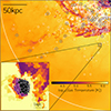 |
Fig. 1. Visualization of the distribution of clouds in a quadrant of our highest resolved GIBLE halo, a Milky Way-like galaxy at z = 0. The center of the galaxy is in the top right corner (main image). The image extends R200c from edge-to-edge, and ±R200c along the projection direction. The colors show mean mass-weighted gas temperatures in projection. The circles show the positions of the many hundred cold dense CGM gas clouds with masses greater than 105 M⊙. Our fiducial sample with Mcl ∼ 106 M⊙ is marked in gray. The inset, a highly zoomed-in region of the halo, shows a slice of the Voronoi mesh centered around a random cloud from our sample, with all member cells outlined by white lines. Despite their small sizes, the clouds (and their interface layers) were resolved with ∼3700 (2550) gas cells, which enabled the study of small-scale phenomena self-consistently evolved in a cosmological context. |
The inset shows a slice of the Voronoi mesh centered around a single cloud. We outlined the cells belonging to the cloud with white lines. The ratio of the physical scales of the two images is ∼60, and so the inset shows a highly zoomed-in region of the main image, but is still well resolved. Simulations of the kind shown here thus enable the study of small-scale cloud phenomena, including formation and evolution, mixing, among others, with clouds self-consistently evolved in the full cosmological context.
In Fig. 2 we show two examples of the topology of magnetic field lines around cool clouds. The two panels show slices of the Voronoi mesh centered around two distinct clouds. Both are oriented such that their velocities, computed as the mass-weighted mean velocity of all cloud member cells, point along the positive x-axis. Both clouds are infalling toward the center of the galaxy, and are at similar galactocentric distances (∼50 kpc). Cells that belong to the clouds (interface layers) are outlined with black (white) lines. Streamlines show the direction of magnetic field lines in this plane, while the background color corresponds to the density of gas. We include three numbers at the top of each panel: the magnetic curvature averaged over all interface gas cells (κ), the ratio of the mean density of the cloud to that of the ambient background3 (i.e., the density contrast, δ), and the modulus of the difference between the cloud velocity and that of the ambient background (i.e., the velocity contrast, vrel).
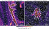 |
Fig. 2. Visualization of the diverse topologies of magnetic field lines around cold CGM clouds. The two panels show slices of the Voronoi mesh centered around two clouds, both oriented such that their mean velocity vector (i.e., the direction of motion) are to the right, the positive x-axis direction. Cells that belong to the cloud (interface layer) are outlined using black (white) lines. Streamlines show the direction of magnetic field lines. The three numbers at the top of each image correspond to the mean magnetic curvature of the cloud interface (κ), the overdensity (δ), and relative velocity (vrel) between the cloud and the interface layer. While the left cloud is threaded by magnetic fields in a region of the background CGM that has particularly uniform field orientation, the magnetic fields in the right panel begin to respond to the motion of the cloud. This diversity is captured by the different values of κ. |
The magnetic field lines around these clouds show contrasting structures. While the field is largely coherent in the left panel, quantified by a relatively low κ of ∼0.1 kpc−1, the topology is more complex on the right with tangled and less laminar field lines (κ ∼ 1.87 kpc−1). The numbers above each panel show that κ correlates with, among other properties, contrasts in both density and velocity, which we consider further in Fig. 4.
In the main panel of Fig. 3 we explore the variation in values of κ across our sample. The black curve corresponds to the computation of κ as the mean over all interface gas cells (i.e., our fiducial definition). The other curves instead compute averages of a sub-selection of interface gas cells from ten bins, constructed based on their relative position in the direction of motion of the cloud, as shown by the colorbar. A relative position of 0.1 would thus correspond to the first 10% of interface gas cells in the direction of motion, 0.2 to the next 10%, and so on.
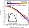 |
Fig. 3. Distribution of interface magnetic curvature values for our sample of Mcl ∼ 106 M⊙ clouds (main panel). The black curve is based on all interface gas, while the other curves show values derived using gas with different relative positions with respect to the direction of motion of the cloud. The purple curves show κ for the head or upstream regions, while the yellow curves show κ in the tail or downstream regions. The inset compares the upstream interface magnetic curvature from our simulations (κGIBLE) to a simple theoretical model (κDP08). |
The black distribution peaks at a value of κ of ≲0.1 kpc−1, is relatively flat out to κ ∼ 0.7 kpc−1, and drops steadily toward higher values. A significant fraction of clouds are thus predicted to have largely coherent fields around them in their interface regions, as in the left panel of Fig. 2. The colored curves show similar behavior, with little dependence on relative position. That is, the degree of curvature does not strongly change between the upstream and downstream interface regions. Previous studies with idealized simulations have shown that field line draping around clouds moving through an initially uniform magnetic field perpendicular to the motion of the cloud is more (less) efficient in the head (tail) (e.g., Jung et al. 2023), corresponding to larger (smaller) values of κ upstream (downstream) of the cloud. The insignificant difference in the distributions of κ between these regions in Fig. 3 suggests that such strong draping configurations are not common around our simulated clouds. We speculate that this is largely due to the background field lines upstream of the cloud not being oriented in perpendicular directions and as uniformly as is typically assumed in idealized setups (see also Sparre et al. 2020). We note here that the distributions explored in Fig. 3 are largely converged up to our RF512 simulations (i.e., eight times lower mass resolution, not shown explicitly).
As the value of κ corresponds to the inverse of the radius of curvature of the local magnetic field, it should scale inversely with the radius of the cloud for strongly draped configurations. However, we checked that the above results are qualitatively similar when values of κ are normalized4 by 1/R (see also the large diversity of κ at fixed R in Fig. 4). The κ distribution therefore reflects physically different field geometries in the cloud interfaces.
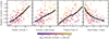 |
Fig. 4. Magnetic curvature (κ) as a function of (from left to right) density contrast between the cloud and its ambient background, vorticity in the interface layer, thermal-to-magnetic pressure ratio of the interface, and cloud radius. The solid curves show the median, while the scatter points correspond to individual clouds, each colored by the velocity contrast between the cloud and its ambient background. A strong trend of κ is seen in the median with respect to each of the properties considered, while the variation of κ at fixed abscissa is typically well captured by the diversity of velocity contrasts of clouds. |
In the inset of Fig. 3, we make a comparison to a simple model describing the expected field around a sphere of radius R moving through a homogeneous ambient medium with an initial uniform magnetic field oriented perpendicular to the cloud motion (Dursi & Pfrommer 2008). Given the assumptions of this model, the solution is not valid in the wake behind the sphere. We thus restrict our comparison to the region around the head of the cloud, which we define using the angular bounds θ = [ − π/3, π/3] and ϕ = [ − π/3, π/3]. Although this choice is arbitrary, we note that adopting other angular ranges for θ and ϕ has no significant impact on the analysis that follows. We compute the theoretical estimate of the model, κDP08, for each cloud separately by setting R to the effective radius of the cloud.
The curve shows the distribution of the ratio κDP08/κGIBLE. The PDF peaks around −0.7, with a large spread, and the model typically underpredicts the curvature seen in the simulation. Although not shown here, we find a weak anti-correlation in this ratio with δ and vrel5, suggesting that the model works better for clouds with relatively small density and velocity contrasts. We speculate that this could be linked to the more efficient build-up of magnetic fields around objects of greater overdensities and velocity contrasts (Lyutikov 2006), thereby increasing the impact of magnetic back-reaction on the flow, which is not considered in the Dursi & Pfrommer (2008) model.
Finally, we return to the correlation between κ and properties of the interface and the ambient background. From left to right, Fig. 4 shows κ as a function of the density contrast (δ), vorticity in the interface layer (ω = ∇ × v), the thermal-to-magnetic pressure ratio of the interface (β), and the radius of the cloud (R). The solid curve shows the median, while the colored points correspond to individual clouds, each colored by vrel. On average, κ increases almost linearly with δ. The scatter clearly correlates with relative velocity: larger values of κ have higher vrel at fixed δ. A linear correlation is also present between κ and ω, indicating a possible connection between a disordered velocity field and a disordered magnetic field. Consistent with theoretical predictions for the case of an initial magnetic field that is coherent on scales larger than the cloud size (McCourt et al. 2015), we find that κ correlates with β. A least-squares fit yields κ ∝ β0.9, roughly in the ballpark of the predicted κ ∝ β trend by Schekochihin et al. (2004) for the case of small-scale turbulent dynamos. While κ decreases with increasing R, the drop is steeper than the 1/R trend expected for a strongly draped configuration (see discussion above), suggesting again that such configurations are not common in our sample. As before, we find that the results shown here are largely converged up to our RF512 level runs.
4. Discussion
The sizes, density contrasts, and kinematics of clouds may thus have an important impact on the structure of ambient field lines. The resulting magnetic field topology may in turn affect cloud growth and evolution. For example, the draped magnetic field layer increases the drag force by a factor of ∼[1 + (vA/vrel)2]≡[1 + (Rκ)−1], where vA is the Alfven speed in the background. The enhanced drag force decreases the “stopping distance” by [1 + (Rκ)−1]−1 (i.e., the distance travelled by the cloud prior to achieving velocity equilibrium with its surroundings), thereby improving the chances of their survivability (McCourt et al. 2015). The diversity of cloud and interface properties portrayed by Fig. 4 suggests that the impact of field line topology on a population of clouds is expected to be varied. Specifically, at fixed R, clouds with lower δ, β and vrel typically have lower values of Rκ, and would thus experience a larger boost in their drag force compared to high δ/β/vrel counterparts6. We reiterate that cosmological simulations like GIBLE allow us to assess such predictions for an actual diverse cloud population since clouds, their interfaces, and their magnetic fields evolve self-consistently.
The magnetic field topology and draped layers may furthermore play a role in suppressing the impact of the Kelvin–Helmholtz instability along the surface of the cloud (e.g., Pfrommer & Dursi 2010). For instance, at fixed Bwind, Sparre et al. (2020) showed that clouds with draped topologies in their interfaces are expected to survive longer. In addition, Jung et al. (2023) find that regions where field lines are inefficiently draped (i.e., low values of κ) fragment rapidly into smaller clumps, while regions of high κ are instead extended into long filamentary structures as a result of enhanced magnetic tension and effectively survive longer. However, it is important to note that the net impact of this suppression of mixing on the evolution of clouds may depend on the efficiency of radiative cooling in the interface layer (e.g., Gronke & Oh 2018). In agreement with idealized work, clouds in TNG50 have temperature gradients into their interfaces (i.e., they are surrounded by a mixed-phase layer of warm gas that rapidly cools onto the cloud; Nelson et al. 2020), consistent with theoretical local cooling flow models (Dutta et al. 2022). Moreover, the metal content of clouds and their interfaces can vary significantly (Nelson et al. 2020; Ramesh et al. 2023a), possibly affecting the rate at which the gas in the interface condenses. Future work will quantify the resulting impact on cloud growth and survival in our simulations with Lagrangian tracers (Ramesh et al., in prep.).
While we find that clouds are roughly in pressure balance with their interface layers (Ramesh et al. 2023a), thereby preventing them from being crushed and dissolved, the TNG model does not include thermal conduction. The inclusion of this component may contribute to cloud evaporation (e.g., Marcolini et al. 2005; Vieser & Hensler 2007), although certain configurations of magnetic fields may partially suppress this effect (Ettori & Fabian 2000; Brüggen et al. 2023). Future simulations that include conduction can explore its role in cosmological cloud evolution. This will require that we adequately resolve the Field length (Field 1965) to avoid spurious numerical effects (Koyama & Inutsuka 2004). For example, for 10% Spitzer conduction (see, e.g., Brüggen et al. 2023) the Field length would be ∼120 pc for interface gas cells, requiring a spatial resolution of ≲40 pc in this region7 (i.e., 2 − 4× better spatial resolution than our current RF4096 run; see Fig. 2 of Ramesh & Nelson 2024).
5. Summary
In this paper we used a cosmological zoom-in galaxy formation simulation with additional CGM refinement to study and explore the complex and diverse topology of magnetic field lines around cold, dense clouds in the CGM. At an average baryonic mass resolution of ∼225 M⊙, the interface layers around our sample of 105.8 < Mcl/M⊙ < 106.2 clouds are resolved by over 2000 resolution elements, allowing the study of interface phenomena in a cosmological context.
We quantified the structure of magnetic field lines around clouds (i.e., in interface layers) by the magnetic curvature κ. We find that values of κ vary significantly, reflecting the diversity in field line topologies around clouds. There is no significant difference in the distribution of κ between the regions upstream and downstream of the cloud, suggesting that strong draping configurations are rare in our sample. However, curvature correlates strongly with cloud-background contrasts in density and velocity: greater contrasts correspond to higher κ, on average. In addition, κ also correlates with other interface properties, including vorticity and the thermal-to-magnetic pressure ratio.
This study provides a first perspective from the point of view of cosmological simulation regarding the topology of magnetic field lines around cold clouds. However, there are several clear avenues to extend this work. In particular, we can assess the impact of cloud motion on the immediate interface layer, and on the broader local gaseous environment of clouds. With Lagrangian tracers we can also quantify the impact of magnetic fields on the lifetime, survival, and evolution of clouds.
While interface gas cells are typically contiguous among themselves, there are rare cases where gaps may be present in the interface.
We exclusively consider the z = 0 simulation snapshot to best connect with the observational Milky Way HVC community.
We define the ambient background as being comprised of three layers of non-cold gas cells around clouds.
Following Nelson et al. (2020), we define the effective radius by the volume equivalent sphere, R = [3Vcloud/4π]1/3.
The value of κ predicted by the Dursi & Pfrommer (2008) model only depends on R, and does not take δ and vrel as input parameters.
This only describes the enhancement factor of the drag force as a result of draping. The total drag force experienced by the cloud (![Mathematical equation: $ {\sim}\rho_{{\rm interface}}^2 {\it v}_{{\rm rel}}^2 R^2 [1 + (R \kappa)^{-1}] $](/articles/aa/full_html/2024/04/aa48786-23/aa48786-23-eq2.gif) ) depends on other properties of the cloud and of the interface.
) depends on other properties of the cloud and of the interface.
This Field condition, that spatial resolution is better than the Field length by at least a factor of 3, was derived using one-dimensional simulations with isotropic conduction (Koyama & Inutsuka 2004).
Acknowledgments
RR and DN acknowledge funding from the Deutsche Forschungsgemeinschaft (DFG) through an Emmy Noether Research Group (grant number NE 2441/1-1). RR is a Fellow of the International Max Planck Research School for Astronomy and Cosmic Physics at the University of Heidelberg (IMPRS-HD). MB acknowledges support from the Deutsche Forschungsgemeinschaft under Germany’s Excellence Strategy – EXC 2121 “Quantum Universe” – 390833306 and from the BMBF ErUM-Pro grant 05A2023. This work has made use of the VERA supercomputer of the Max Planck Institute for Astronomy (MPIA), and the COBRA supercomputer, both operated by the Max Planck Computational Data Facility (MPCDF), and of NASA’s Astrophysics Data System Bibliographic Services.
References
- Banda-Barragán, W. E., Parkin, E. R., Federrath, C., Crocker, R. M., & Bicknell, G. V. 2016, MNRAS, 455, 1309 [CrossRef] [Google Scholar]
- Berlok, T., & Pfrommer, C. 2019, MNRAS, 489, 3368 [NASA ADS] [CrossRef] [Google Scholar]
- Böckmann, K., Brüggen, M., Heesen, V., et al. 2023, A&A, 678, A56 [NASA ADS] [CrossRef] [EDP Sciences] [Google Scholar]
- Boozer, A. H. 2005, Rev. Mod. Phys., 76, 1071 [NASA ADS] [CrossRef] [Google Scholar]
- Brüggen, M., Scannapieco, E., & Grete, P. 2023, ApJ, 951, 113 [CrossRef] [Google Scholar]
- Das, H. K., & Gronke, M. 2024, MNRAS, 527, 991 [Google Scholar]
- Donahue, M., & Voit, G. M. 2022, Phys. Rep., 973, 1 [NASA ADS] [CrossRef] [Google Scholar]
- Dursi, L. J., & Pfrommer, C. 2008, ApJ, 677, 993 [NASA ADS] [CrossRef] [Google Scholar]
- Dutta, A., Sharma, P., & Nelson, D. 2022, MNRAS, 510, 3561 [NASA ADS] [CrossRef] [Google Scholar]
- Ettori, S., & Fabian, A. C. 2000, MNRAS, 317, L57 [CrossRef] [Google Scholar]
- Field, G. B. 1965, ApJ, 142, 531 [Google Scholar]
- Fielding, D. B., Ostriker, E. C., Bryan, G. L., & Jermyn, A. S. 2020, ApJ, 894, L24 [Google Scholar]
- Fielding, D. B., Ripperda, B., & Philippov, A. A. 2023, ApJ, 949, L5 [NASA ADS] [CrossRef] [Google Scholar]
- Girichidis, P. 2021, MNRAS, 507, 5641 [NASA ADS] [CrossRef] [Google Scholar]
- Gronke, M., & Oh, S. P. 2018, MNRAS, 480, L111 [Google Scholar]
- Grønnow, A., Tepper-García, T., Bland-Hawthorn, J., & Fraternali, F. 2022, MNRAS, 509, 5756 [Google Scholar]
- Heesen, V., O’Sullivan, S. P., Brüggen, M., et al. 2023, A&A, 670, L23 [NASA ADS] [CrossRef] [EDP Sciences] [Google Scholar]
- Hidalgo-Pineda, F., Farber, R. J., & Gronke, M. 2024, MNRAS, 527, 135 [Google Scholar]
- Jung, S. L., Grønnow, A., & McClure-Griffiths, N. M. 2023, MNRAS, 522, 4161 [NASA ADS] [CrossRef] [Google Scholar]
- Klein, R. I., McKee, C. F., & Colella, P. 1994, ApJ, 420, 213 [Google Scholar]
- Koyama, H., & Inutsuka, S.-I. 2004, ApJ, 602, L25 [CrossRef] [Google Scholar]
- Kwak, K., Shelton, R. L., & Raley, E. A. 2009, ApJ, 699, 1775 [NASA ADS] [CrossRef] [Google Scholar]
- Lyutikov, M. 2006, MNRAS, 373, 73 [CrossRef] [Google Scholar]
- Marcolini, A., Strickland, D. K., D’Ercole, A., Heckman, T. M., & Hoopes, C. G. 2005, MNRAS, 362, 626 [NASA ADS] [CrossRef] [Google Scholar]
- Marinacci, F., Vogelsberger, M., Pakmor, R., et al. 2018, MNRAS, 480, 5113 [NASA ADS] [Google Scholar]
- McCourt, M., O’Leary, R. M., Madigan, A.-M., & Quataert, E. 2015, MNRAS, 449, 2 [NASA ADS] [CrossRef] [Google Scholar]
- Mellema, G., Kurk, J. D., & Röttgering, H. J. A. 2002, A&A, 395, L13 [NASA ADS] [CrossRef] [EDP Sciences] [Google Scholar]
- Muller, C. A., Oort, J. H., & Raimond, E. 1963, Acad. Sci. Paris Comptes Rendus, 257, 1661 [NASA ADS] [Google Scholar]
- Nelson, D., Pillepich, A., Springel, V., et al. 2018, MNRAS, 475, 624 [Google Scholar]
- Nelson, D., Sharma, P., Pillepich, A., et al. 2020, MNRAS, 498, 2391 [NASA ADS] [CrossRef] [Google Scholar]
- Pakmor, R., & Springel, V. 2013, MNRAS, 432, 176 [NASA ADS] [CrossRef] [Google Scholar]
- Pakmor, R., Marinacci, F., & Springel, V. 2014, ApJ, 783, L20 [CrossRef] [Google Scholar]
- Pakmor, R., van de Voort, F., Bieri, R., et al. 2020, MNRAS, 498, 3125 [NASA ADS] [CrossRef] [Google Scholar]
- Pfrommer, C., & Dursi, J. 2010, Nat. Phys., 6, 520 [NASA ADS] [CrossRef] [Google Scholar]
- Pfrommer, C., Werhahn, M., Pakmor, R., Girichidis, P., & Simpson, C. M. 2022, MNRAS, 515, 4229 [NASA ADS] [CrossRef] [Google Scholar]
- Pillepich, A., Springel, V., Nelson, D., et al. 2018, MNRAS, 473, 4077 [Google Scholar]
- Powell, K. G., Roe, P. L., Linde, T. J., Gombosi, T. I., & De Zeeuw, D. L. 1999, J. Comput. Phys., 154, 284 [NASA ADS] [CrossRef] [Google Scholar]
- Ramesh, R., & Nelson, D. 2024, MNRAS, 528, 3320 [NASA ADS] [CrossRef] [Google Scholar]
- Ramesh, R., Nelson, D., & Pillepich, A. 2023a, MNRAS, 522, 1535 [NASA ADS] [CrossRef] [Google Scholar]
- Ramesh, R., Nelson, D., Heesen, V., & Brüggen, M. 2023b, MNRAS, 526, 5483 [NASA ADS] [CrossRef] [Google Scholar]
- Ramesh, R., Nelson, D., & Pillepich, A. 2023c, MNRAS, 518, 5754 [Google Scholar]
- Scannapieco, E., & Brüggen, M. 2015, ApJ, 805, 158 [NASA ADS] [CrossRef] [Google Scholar]
- Schekochihin, A. A., Cowley, S. C., Taylor, S. F., Maron, J. L., & McWilliams, J. C. 2004, ApJ, 612, 276 [NASA ADS] [CrossRef] [Google Scholar]
- Shen, C., Li, X., Dunlop, M., et al. 2003, J. Geophys. Res. (Space Phys.), 108, 1168 [NASA ADS] [CrossRef] [Google Scholar]
- Shin, M.-S., Stone, J. M., & Snyder, G. F. 2008, ApJ, 680, 336 [NASA ADS] [CrossRef] [Google Scholar]
- Sparre, M., Pfrommer, C., & Ehlert, K. 2020, MNRAS, 499, 4261 [NASA ADS] [CrossRef] [Google Scholar]
- Springel, V. 2010, MNRAS, 401, 791 [Google Scholar]
- Springel, V., White, S. D. M., Tormen, G., & Kauffmann, G. 2001, MNRAS, 328, 726 [Google Scholar]
- Vieser, W., & Hensler, G. 2007, A&A, 472, 141 [NASA ADS] [CrossRef] [EDP Sciences] [Google Scholar]
- Wakker, B. P., & van Woerden, H. 1997, ARA&A, 35, 217 [NASA ADS] [CrossRef] [Google Scholar]
- Weinberger, R., Springel, V., Hernquist, L., et al. 2017, MNRAS, 465, 3291 [Google Scholar]
All Figures
|
Fig. 1. Visualization of the distribution of clouds in a quadrant of our highest resolved GIBLE halo, a Milky Way-like galaxy at z = 0. The center of the galaxy is in the top right corner (main image). The image extends R200c from edge-to-edge, and ±R200c along the projection direction. The colors show mean mass-weighted gas temperatures in projection. The circles show the positions of the many hundred cold dense CGM gas clouds with masses greater than 105 M⊙. Our fiducial sample with Mcl ∼ 106 M⊙ is marked in gray. The inset, a highly zoomed-in region of the halo, shows a slice of the Voronoi mesh centered around a random cloud from our sample, with all member cells outlined by white lines. Despite their small sizes, the clouds (and their interface layers) were resolved with ∼3700 (2550) gas cells, which enabled the study of small-scale phenomena self-consistently evolved in a cosmological context. |
| In the text | |
|
Fig. 2. Visualization of the diverse topologies of magnetic field lines around cold CGM clouds. The two panels show slices of the Voronoi mesh centered around two clouds, both oriented such that their mean velocity vector (i.e., the direction of motion) are to the right, the positive x-axis direction. Cells that belong to the cloud (interface layer) are outlined using black (white) lines. Streamlines show the direction of magnetic field lines. The three numbers at the top of each image correspond to the mean magnetic curvature of the cloud interface (κ), the overdensity (δ), and relative velocity (vrel) between the cloud and the interface layer. While the left cloud is threaded by magnetic fields in a region of the background CGM that has particularly uniform field orientation, the magnetic fields in the right panel begin to respond to the motion of the cloud. This diversity is captured by the different values of κ. |
| In the text | |
|
Fig. 3. Distribution of interface magnetic curvature values for our sample of Mcl ∼ 106 M⊙ clouds (main panel). The black curve is based on all interface gas, while the other curves show values derived using gas with different relative positions with respect to the direction of motion of the cloud. The purple curves show κ for the head or upstream regions, while the yellow curves show κ in the tail or downstream regions. The inset compares the upstream interface magnetic curvature from our simulations (κGIBLE) to a simple theoretical model (κDP08). |
| In the text | |
|
Fig. 4. Magnetic curvature (κ) as a function of (from left to right) density contrast between the cloud and its ambient background, vorticity in the interface layer, thermal-to-magnetic pressure ratio of the interface, and cloud radius. The solid curves show the median, while the scatter points correspond to individual clouds, each colored by the velocity contrast between the cloud and its ambient background. A strong trend of κ is seen in the median with respect to each of the properties considered, while the variation of κ at fixed abscissa is typically well captured by the diversity of velocity contrasts of clouds. |
| In the text | |
Current usage metrics show cumulative count of Article Views (full-text article views including HTML views, PDF and ePub downloads, according to the available data) and Abstracts Views on Vision4Press platform.
Data correspond to usage on the plateform after 2015. The current usage metrics is available 48-96 hours after online publication and is updated daily on week days.
Initial download of the metrics may take a while.