| Issue |
A&A
Volume 684, April 2024
|
|
|---|---|---|
| Article Number | A166 | |
| Number of page(s) | 23 | |
| Section | Extragalactic astronomy | |
| DOI | https://doi.org/10.1051/0004-6361/202347522 | |
| Published online | 19 April 2024 | |
The debiased morphological transformations of galaxies since z = 3 in CANDELS
1
Department of Astronomy, Universidad de Concepcion, Casilla 160-C Concepción, Chile
e-mail: This email address is being protected from spambots. You need JavaScript enabled to view it.
2
Department of Computer Engineering, Universidad de Concepcion, Casilla 160-C Concepción, Chile
Received:
20
July
2023
Accepted:
6
January
2024
Abstract
Context. Morphological quantitative measurements and visual-like classifications are susceptible to biases arising from the expansion of the Universe. One of these biases is the effect of cosmological surface brightness dimming (CSBD): the measured surface brightness of a galaxy decays with redshift as (1 + z)−4. This effect might lead an observer to perceive an altered morphology compared to the real one.
Aims. Our goal is to investigate the impact of CSBD on morphological classifications to determine the true evolution of morphological classes over redshift for field galaxies, and to interpret these results in the context of morphological transformations and star formation quenching.
Methods. We employed artificial redshifting techniques on a sample of 268 galaxies in the five CANDELS fields, spanning redshifts from z = 0.2 to z = 3.0. We compared the visual classifications and morphological coefficients (G, M20, and As) obtained from the original and simulated images. Subsequently, we developed two correction methods to mitigate the effects of CSBD.
Results. Our findings reveal that CSBD, low resolution, and signal-to-noise significantly bias the visual morphological classifications beyond z > 1. Specifically, we observed an overestimation of the fractions of spheroids and irregular galaxies by up to 50%, while the fractions of early- and late-type disks were underestimated by 10% and 50%, respectively. However, we found that morphological coefficients are not significantly affected by CSBD at z < 2.25. We validated the consistency of our correction methods by applying them to the observed morphological fractions in the IllustrisTNG-50 sample and comparing them to previous studies.
Conclusions. We propose two potential sources of confusion regarding the visual classifications due to CSBD. Firstly, galaxies may be misclassified as spheroids, as the dimming effect primarily renders the bulge component visible. Secondly, galaxies may be misidentified as irregulars due to their more diffuse and asymmetric appearance at high redshifts. By analyzing the morphological fractions of star-forming and quiescent subsamples as a function of redshift and stellar mass, we propose a scenario where late-type disks transform into quiescent spheroids through mergers or to early-type disks through secular evolution or active galactic nucleus feedback.
Key words: galaxies: evolution / galaxies: fundamental parameters / galaxies: structure
© The Authors 2024
 Open Access article, published by EDP Sciences, under the terms of the Creative Commons Attribution License (https://creativecommons.org/licenses/by/4.0), which permits unrestricted use, distribution, and reproduction in any medium, provided the original work is properly cited.
This article is published in open access under the Subscribe to Open model. This email address is being protected from spambots. You need JavaScript enabled to view it. to support open access publication.
1. Introduction
Galaxies are baryonic and dark matter over-densities that have been or are capable of transforming cold molecular gas into stars (Huertas-Company et al. 2016). The star formation rate (SFR) of a galaxy depends on whether internal and external processes that act in favor of star formation (e.g., gas inflow and cooling) dominate over the processes that halt it – for example, active galactic nucleus (AGN) feedback and gas heating – or vice versa. The well-known star formation rate density (SFRD) versus redshift (z) diagram shown by Madau & Dickinson (2014) shows that the Universe reaches a star formation peak around z ∼ 2 and subsequently experiences a decrease until present times. The latter is due to quenching processes (Renzini 2016) and lower molecular gas fractions at low redshifts (Gobat et al. 2020). Despite the ubiquity of this trend, the details of the physical processes that drive quenching remain elusive and require further investigation.
Regardless of whether galaxies cease star formation, their stellar populations continue to evolve. The evolution of the stellar populations of both star-forming and quenched galaxies results in a well-defined galaxy bimodality in a color-magnitude diagram. Specifically, the star-forming galaxies congregate in the demarcated blue cloud, while the passive, non-star-forming galaxies are clustered in the so-called red sequence (Strateva et al. 2001; Baldry et al. 2004). Moreover, when examining the relationship between the SFR and the stellar mass (M*) of galaxies, those that are actively forming stars generally populate a main sequence that lies above a region occupied by passive galaxies.
Observational investigations (e.g., Christlein & Zabludoff 2005; Bruce et al. 2012; Wang et al. 2012; Lee et al. 2013) have demonstrated that there is a link between the morphology of galaxies and their star formation activity. Explicitly, star-forming galaxies that populate the main sequence and the blue cloud typically have disk-like shapes, while passive galaxies that lack ongoing star formation and predominantly occupy the red sequence exhibit a dominant spheroidal morphology. This link underscores how the morphology of galaxies, a property that refers to their shape and light distribution, is interconnected with other physical properties, including color and SFR (Brennan et al. 2015).
There is abundant evidence (e.g., Hausman & Ostriker 1978; Abraham & van den Bergh 2001; van Dokkum & Franx 2001; Postman et al. 2005; Genzel et al. 2008; van der Wel 2008; Cerulo et al. 2017) on the evolution of the morphological mixing of galaxies with time. In the local Universe, galaxies are predominantly bulge-dominated (elliptical and lenticular, which are known together as early-type), whereas at z = 3, approximately 80% of galaxies exhibit disk-like morphologies (late-type). The fraction of disk-dominated galaxies declines to approximately 20% in the nearby Universe as noted by Conselice et al. (2004), Delgado-Serrano et al. (2010), Conselice (2014). These findings motivate us to explore the potential links between the mechanisms that trigger or quench star formation and the morphological transformations of galaxies.
The evolution of galaxies is driven by physical mechanisms that may originate within the galaxies, as in the case of the AGN and supernova feedback, or that are related to the environment that surrounds them (see e.g., Peng et al. 2010; van der Burg et al. 2020). Thus, the simultaneous study of galaxies in different environments, such as those of clusters and the field, is important to infer the relevance of the different processes that are responsible for the transformation of their properties. It is for this reason that we have embarked on a study of the relationships between morphology and star formation in cluster and field galaxies with the aims of reconstructing the evolutionary paths of galaxies with different morphologies and inferring the links between morphological transformations and star formation quenching. While the present paper focuses on field galaxies, a parallel paper that is currently in preparation (Cerulo et al., in prep.) focuses on galaxy clusters at z = 0.2 − 0.9.
Any study of the morphology of galaxies should take into account that the expansion of the Universe and the presence of the intergalactic medium affect the transmission of the light from a source to an observer on Earth. There are two main sources of bias that can arise from cosmic expansion, namely the morphological K correction and the dimming of the observed surface brightness. The first arises from the fact that distant sources are sampled at rest-frame wavelengths that are bluer than those at which they are observed. This implies that there is a contribution to the difference between the morphology of distant and nearby galaxies that results from the fact that the stellar populations sampled at high and low redshifts are different (Windhorst et al. 2009; Buta 2011). The bias arising from the morphological K correction is corrected by choosing a set of filters for the classification of galaxies that allows similar stellar populations to be sampled.
The second observational bias arises from the fact that as a consequence of the expansion of the Universe, the observed surface brightness of a source decreases according to a power law of the type (1 + z)−4 – cosmological surface brightness dimming (CSBD; Tolman 1930). This means that distant galaxies appear more diffuse than their nearby counterparts, regardless of the filter used for observations. This effect, combined with the extinction by the intergalactic medium and the loss of resolution as the projected size of a galaxy approaches the full width at half maximum (FWHM) of the point spread function (PSF), implies that high-z galaxies appear smaller overall, more diffuse, and less resolved with respect to galaxies in the local Universe.
Most of the literature on CSBD primarily focuses on the contribution of this phenomenon to the selection (Malmquist) bias, which is the systematic preference to detect only high surface brightness galaxies at high redshift (e.g., Bouwens et al. 2004; Calvi et al. 2014; Paulino-Afonso et al. 2017). However, there is limited discussion on the impact of CSBD on morphology (Barden et al. 2008; Mortlock et al. 2013; Willett et al. 2017). As a part of this study, we aim to evaluate the significance of the CSBD bias on the morphological classification of galaxies. This is crucial to determine whether it is necessary to decouple the effect of CSBD to retrieve the actual morphological evolution of galaxies.
This paper presents two methods for the assessment and evaluation of the CSBD bias, which are both based on the artificial redshifting of galaxies. The first is aimed at studying the effect of CSBD on visual classification, while the other investigates its effect on the classification based on nonparametric coefficients. The software DOPTERIAN (Paulino-Afonso et al. 2017) was employed to simulate high-z observations of nearby galaxies.
For this paper the CSBD corrections were applied to a sample of 23,088 galaxies from the Cosmic Assembly Near-Infrared Deep Extragalactic Legacy Survey (CANDELS, Grogin et al. 2011; Koekemoer et al. 2011) at redshifts z = 0.2 − 3.0, and the results were compared with the predictions of the IllustrisTNG-50 (TNG50) simulation (Nelson et al. 2019; Pillepich et al. 2019). The results obtained from this study provide a quantitative assessment of the relevance of CSBD in the morphological classification of galaxies, as well as a method to correct galaxy morphology for this effect.
The paper is organized as follows. Section 2 introduces the dataset used in the study, including the sample of galaxies, the images, and the simulations. In Sect. 3 the methods employed to derive and correct the morphological fractions for CSBD are outlined and the results of the analysis are presented. Section 4 provides a comprehensive discussion and interpretation of the results, which are summarized in Sect. 5.
Throughout the paper magnitudes are given in the AB system (Oke & Gunn 1983). We assume a Λ-cold dark matter (ΛCDM) cosmological model with H0 = 70.0 km⋅s−1⋅Mpc−1, Ωm = 0.3, and ΩΛ = 0.7.
2. The data: Images and simulations
With the purpose of studying low-density environments, we built a sample from the five fields of the Cosmic Assembly Near-infrared Deep Extragalactic Legacy Survey, CANDELS (Grogin et al. 2011; Koekemoer et al. 2011). CANDELS is an observational program that obtained deep images (mosaics) of the Great Observatories Origins Deep Survey North and South (GOODS-N and GOODS-S, Giavalisco et al. 2004), Extended Groth Strip (EGS, Davis et al. 2007), Cosmic Evolution Survey (COSMOS, Scoville et al. 2007), and the UKIRT1 Infrared Deep Sky Survey (UKIDSS) Ultra-deep Survey field (UDS, Lawrence et al. 2007) fields using the Hubble Space Telescope (HST) Wide-field Camera 3 (WFC3) and Advanced Camera for Surveys (ACS) over a period of 902 orbits.
CANDELS was chosen for this study for three main reasons, namely its large area (∼130 arcmin2 and ∼720 arcmin2 in its deep-mode and wide-mode, respectively, containing images of more than 250 000 galaxies), its deep photometric F160W limit (H = 27.0 mag), and its wide usage in the astronomical community which enables the results of this paper to be compared with other works in the recent literature. Furthermore, as the CANDELS fields have been extensively studied in the last decade, several ancillary catalogs containing photometric and spectroscopic redshifts, stellar masses, SFRs and morphological parameters are publicly available. Our CANDELS sample includes all galaxies in the redshifts range z = 0.4 − 3.0 with H ≤ 24.5, which yielded a total of 23 088 galaxies with stellar masses ranging from log(M*) = 9.00 to log(M*) = 12.00.
We use the visual-like morphological classifications published with Huertas-Company et al. (2015), who utilized a convolutional neural network (CNN) architecture to classify all objects in the five CANDELS fields. The CNN algorithm was trained on the sample of visual morphologies published in Kartaltepe et al. (2015) and estimated for each object a set of numbers between 0 and 1, corresponding to the frequencies with which a hypothetical team of classifiers would assign it to one of the morphological classes defined in Kartaltepe et al. (2015): dominant spheroid (fsph), dominant disk (fdisk), dominant irregular (firr), dominant point source (fps), and unclassifiable (func). To convert the set of five morphological frequencies to a single morphological class label, we followed the criterion proposed in Huertas-Company et al. (2016):
-
Spheroid:fsph > 2/3 and fdisk < 2/3 and firr < 1/10.
-
Late-type disk:fsph < 2/3 and fdisk > 2/3 and firr < 1/10.
-
Early-type disk:fsph > 2/3 and fdisk > 2/3 and firr < 1/10.
-
Irregular:fsph < 2/3 and firr > 1/10.
As explained in Huertas-Company et al. (2016), the thresholds are calibrated on visual inspection to make sure that the intervals corresponded to distinct morphological classes.
2.1. Reference sample
In order to quantify the impact of CSBD and to develop effective correction methods, we constructed a reference sample that comprises 268 galaxies with H ≤ 22 mag randomly selected from all CANDELS fields and located at z = 0.2 − 0.4. The magnitude limit was chosen so that simulations are conducted on the brightest objects within the CANDELS bin 0. If less bright galaxies were used, the majority of objects would end up being unclassifiable. The physical properties of the galaxies of the reference sample, such as their coordinates, stellar mass, bulge mass, Sérsic indices, redshift, SFR, and others, were obtained from the catalog of the 3D-HST Treasury Program (Momcheva et al. 2016)2.
We used the mosaics of each field, retrieved from the 3D-HST repository (Grogin et al. 2011; Koekemoer et al. 2011; Brammer et al. 2012; Skelton et al. 2014; Momcheva et al. 2016)3, to visually classify all objects in the reference sample. The visual classification was carried out on postage stamp images centered on the galaxies and having sizes equal to four times the geometric mean of the semi-major and semi-minor axis of the Petrosian ellipse4.
2.2. Simulations of high-redshift observations
The expansion of the Universe causes the observed surface brightness of a galaxy to decrease according to the equation:
 (1)
(1)
where Σ is the rest-frame surface brightness. As mentioned earlier, the dimming effect causes distant galaxies to seem more diffuse than closer ones. This can lead to misclassification of a galaxy’s morphology.
To assess the relevance of CSBD in morphological classification, we produced redshifted versions of the galaxies of the reference sample with the software DOPTERIAN (Paulino-Afonso et al. 2017), which is a Python implementation of the Interactive Data Language (IDL) routine Full and Efficient Redshifting of Ensembles of Nearby Galaxy Images (FERENGI, Barden et al. 2008). DOPTERIAN simulates high-redshift observations of low-redshift galaxies by accounting for changes in the angular size and surface brightness of the source. The simulation process is divided in four steps:
-
The input image, of pixel size pi (angular size of the pixel in arcseconds), is modified for cosmological effects (i.e., changes in the source’s angular size and surface brightness) by re-binning the image into an output-image of pixel size pf, while preserving the galaxy’s physical scale and the image total flux.
-
The flux of each pixel is scaled to correct for the effect of surface brightness dimming, as described in Eq. (1).
-
A PSF convolution kernel is created to compensate for the differences between the input and output PSFs. This step is critical, since with the shrinking and degrading of the images performed in the previous two steps, the original PSF is also shrunk. The output and shrunken input PSFs are transformed into the Fourier space and the spectrum of the former is divided by that of the latter. This is equivalent to a deconvolution of the output PSF by the shrunken input PSF. The obtained spectrum is transformed back to the spatial domain, providing in this way the convolution kernel for the degraded image.
-
The kernel is convolved with the corrected and rescaled image. Poisson noise is added randomly, and the galaxy is then placed on top of an image of an empty patch of the sky derived from the original image.
The simulations also incorporate changes in resolution and signal-to-noise ratio. For further details and information on the working procedures of DOPTERIAN and FERENGI, the reader is referred to the works of Paulino-Afonso et al. (2017) and Barden et al. (2008), respectively.
Each postage stamp was simulated at random redshifts within six predefined redshift bins, resulting in six artificially redshifted versions of each of the 268 galaxies in the reference sample. The ranges of each redshift bin are shown in Table 1. The mean or intermediate z is used as the representative redshift for each bin. From now onward, we use the terms reference sample and original sample interchangeably when referring to the 268 galaxy images that have not been artificially redshifted.
Intervals (bins) used for galaxy redshifting.
Since distant galaxies are intrinsically brighter, we increased the flux of the simulated galaxies by an amount equal to the difference between the medians of the magnitude distributions of real and simulated galaxies in each redshift bin (see e.g., Conselice 2003, Mortlock et al. 2013 and Willett et al. 2017). Figures 1 and 2 plot a comparison between the distribution of magnitudes and signal-to-noise (S/N) for both the CANDELS dataset and the reference sample, respectively. Ten examples of the simulations are illustrated in Fig. 3.
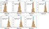 |
Fig. 1. Comparative histogram illustrating the magnitude distributions of the CANDELS dataset (blue) and the reference sample (orange) across all redshift bins. Each panel displays the result of the two-sample Kolmogorov-Smirnov test. The magnitude was estimated with SExtractor. |
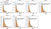 |
Fig. 2. Histograms illustrating the signal-to-noise (S/N) distributions of the CANDELS dataset (blue) and the reference sample (orange) across all redshift bins. Each panel displays the result of the two-sample Kolmogorov-Smirnov test. The S/N was measured with SExtractor. |
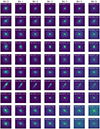 |
Fig. 3. Postage stamp images of ten galaxies from the reference sample alongside their simulated counterparts across all redshift bins. The pixel scale of each stamp varies while maintaining the physical scale of the image. The change with redshift of the aspect of the galaxies can be appreciated. |
In order to take into account the effects of the morphological K-correction, we chose the filters that would be closest to the rest-frame wavelength in each redshift bin and used the postage stamps derived from the corresponding images to redshift the galaxies. The filters used for each redshift bin are outlined in Table 2, where it can be noted that not all CANDELS fields have the same set of optical filters.
Filters used to produce redshifted images of z = 0.2 − 0.4 CANDELS galaxies.
2.3. The comparison sample: The Illustris-TNG50 simulation
According to the ΛCDM cosmological paradigm, the initial structures in the Universe formed from matter over-densities where gravitational collapse led to the condensation of matter and the emergence of small structures (Abel et al. 1998; Ryden & Gunn 1987). Galaxy formation is often theorized as a hierarchical process, with smaller structures merging over time (Cole et al. 2000). However, the intricate details of galaxy evolution involve complex interplays of physical processes, including gravitational, radiative, hydrodynamical, and magnetic effects, such as star formation, gas cooling, chemical enrichment, and feedback mechanisms like supernovae and AGN. Analytical models and numerical simulations, like the Illustris simulation (Genel et al. 2014; Vogelsberger et al. 2014a,b), aim to capture these complexities, providing insights into the Universe’s evolution by considering large-scale magneto-hydrodynamic simulations incorporating gravity, fluid dynamics, magnetic fields, and the formation of structures, such as stars, galaxies, and black holes.
The present study has employed the highest resolution product of the IllustrisTNG project, namely the TNG50 simulation (Nelson et al. 2019; Pillepich et al. 2019), which consists of a simulated cube with sides of 50 Mpc. The choice of this particular version of the simulation was motivated by the availability of morphological measurements of some of the galaxies in the associated supplementary data catalogs. These catalogs were published by Huertas-Company et al. (2019) and Varma et al. (2022), who used a CNN model similar to that of Huertas-Company et al. (2015) to perform the morphological classification of galaxies. Specifically, they classified galaxies in six snapshots (25, 29, 33, 40, 50, and 67) of the TNG50 simulation, corresponding to redshifts z = 3.0, 2.4, 2.0, 1.5, 1.0 and 0.5, respectively. The algorithm was applied to synthetic CANDELS-like galaxy images, that mimic the properties, depth, and resolution of a CANDELS-like observational sample, generated from the TNG50 products with the SKIRT radiative transfer code (Baes et al. 2011).
The catalog provides the frequencies for each galaxy to belong to one of three major morphological classes, namely dominant disks (fdisk), dominant spheroids (fsph), and irregular (firr). We use these frequencies to obtain a single dominant class label for each galaxy in our study, following the criterion of Varma et al. (2022):
-
Spheroid: if fsph > 0.5 and fdisk < 0.5.
-
Early-type disk: if fsph > 0.5 and fdisk > 0.5 and firr < 0.5.
-
Late-type disk: if fsph < 0.5 and fdisk > 0.5 and firr < 0.5.
-
Irregular:firr > 0.5.
The resulting simulation sample comprises a total of 10 487 galaxies with stellar masses in the range 9.0 < log(M*/M⊙) < 12.0.
2.4. Star-forming and quiescent galaxies
To divide the CANDELS and TNG50 samples into star-forming and quiescent galaxies, we used a cut in log10(SFR). To account for the evolution of the SFR of main-sequence galaxies with redshift, we adopted the parametrization provided by Schreiber et al. (2015):
![Mathematical equation: $$ \begin{aligned} \log _{10}(SFR_{\rm MS}[M_\odot /\mathrm{yr}]) = m-m_0+a_0r-a_1[\max (0,m-m_1-a_2r)]^2, \end{aligned} $$](/articles/aa/full_html/2024/04/aa47522-23/aa47522-23-eq2.gif) (2)
(2)
where r ≡ log10(1 + z), m ≡ log10(M*/109 M⊙), m0 = 0.5 ± 0.07, a0 = 1.5 ± 0.15, a1 = 0.3 ± 0.08 and m1 = 0.36 ± 0.3 and a2 = 2.5 ± 0.6.
Assuming that galaxies along this main-sequence follow a normal SFR distribution with standard deviation σSFR, we initially considered that all galaxies that were 3σSFR below the main sequence were quiescent. In the resulting star-forming sample, we fit a nonparametric curve using a Gaussian process. Then we split again the sample into star-forming and quiescent galaxies using the updated value σ* for the standard deviation about the main sequence. We again defined as quiescent every galaxy that was below 3σ*. We repeated the nonparametric fit and 3-σ clipping until no more objects were removed from the star-forming subsample and added to the quiescent subsample.
3. Methods and results
To investigate the impact of CSBD on the estimation of morphological fractions, we developed two approaches for quantifying and correcting this effect. The first approach is based on the comparison between the visually classified morphologies of the galaxies of the reference sample and of their redshifted versions. The second approach is based on the characterization of galaxy morphology in the space formed by the Gini coefficient (G), the second order moment of the light distribution (M20) and the asymmetry coefficient (As).
Before explaining the two methods, it is important to introduce the morphological scheme used for the visual classification of the galaxies in the reference sample. We visually classified galaxies into five morphological classes: spheroids, lenticulars/early-type disks, late-type disks, irregulars and point sources/unclassifiable/artifacts. This division was chosen to align our results with those of previous studies (e.g., Kartaltepe et al. 2015; Huertas-Company et al. 2016, 2023; Cerulo et al. 2017; Varma et al. 2022; Jacobs et al. 2023). Morphological classes are defined below.
Spheroids. Galaxies with a smooth and round/elliptical appearance that is centrally concentrated. This class includes only ellipticals.
Early-type disks. Galaxies with a distinct flat disk structure that may or may not exhibit visible spiral arms. They also feature a significant central bulge. This class includes Sa and Sb spirals and lenticulars.
Late-type disks. Galaxies with a distinct flat disk structure that may or may not exhibit visible spiral arms. The also feature a small or no bulge. This class includes Sc and Sd spirals.
Irregulars. Objects that do not have a regular structure, are neither spheroidal nor have a disk-dominated morphology. They may exhibit asymmetries, tidal tails, merging features, or other signs of morphological disturbances.
Point sources and unclassifiable. Point sources are round-like sources whose internal structure cannot be resolved due to their small size. On the other hand, objects may be labeled as unclassifiable due to a variety of reasons such as image issues (e.g., satellite trails, proximity to a bright star or galaxy, etc.), spuriousness of the object (e.g., part of a diffraction spike), or extreme faintness of the object that makes it impossible to discern any structure.
We eliminated from the reference sample all objects that were categorized as unclassifiable/artifacts or point sources in any given redshift bin. As a result of these modifications, the reference sample was reduced to 256 objects.
3.1. Morphological fractions
The morphological fractions are defined as the ratio of the number of objects of a specific morphological type to the total number of objects considered within each redshift bin. In a statistical framework, these fractions can be understood as the success rate proportion in a Bernoulli probability distribution. Here, the number of objects belonging to the target morphological type is considered as the successes, while the total number of objects in the redshift or stellar mass bin is the sample size, that is, the total number of trials.
The morphological fractions can be interpreted as the population proportion in a hypothetical experiment in which k galaxies of a given morphological type are randomly drawn from a sample of n galaxies. Following Cameron (2011), we consider the mean of the Beta distribution as the best estimator for the morphological fractions and we adopt a confidence level of ±68% for the estimation of the uncertainties on the fractions. In the extreme cases k = 0 and k = 1 we take the median of the distribution as the estimate for the fractions.
Number counts in limited regions of the sky such as those probed in the CANDELS survey may be affected by cosmic variance. We estimated the cosmic variance and Poisson noise budget for each redshift bin in the reference and the CANDELS samples using the method described in Trenti & Stiavelli (2008) and implemented in an on-line calculator. Calculations indicate that cosmic variance is unlikely to significantly impact number counts in both samples.
3.2. Visual classifications (method 1)
A pair of classifiers (DS and PC)5 conducted each an independent visual inspection of the postage-stamp images of the original and redshifted galaxies in the reference sample. The dominant class for each galaxy was determined by the mode of the classification votes. If there was no mode, the classification performed by DS was chosen as the dominant class. The results of the visual classifications can be found in Table 3.
Morphological counts for each redshift bin in the reference sample.
The change in the morphological type for galaxies initially assigned to the same morphological class in bin 0 is shown in Fig. 4. For instance, in the upper left panel of the figure it can be seen the change for all galaxies classified as spheroids in bin 0. The plot helps visualizing the number of galaxies that were misclassified in each redshift bin. For a considerable portion of galaxies (85.16%), the visual morphological type undergoes changes with redshift due to CSBD. It is evident that at higher redshifts there is noticeable confusion between true early-type disk galaxies and spheroids, while true late-type disks tend to be confused with all the other classes. True irregular galaxies, on the other hand, are predominantly misidentified as spheroids and early-type disks. Notably, true spheroids exhibit minimal confusion across all redshifts.
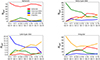 |
Fig. 4. Effect of CSBD on the visual classification. Each panel displays all galaxies in the reference sample that share a morphological label in bin 0. This diagram provides a representation of the different channels of confusion in the visual classification of distant galaxies. |
The misclassification may be primarily attributed to two confusion channels: galaxies tend to either look more bulge-dominated or their apparent structure becomes more irregular. The former channel likely accounts for irregulars, early-type and late-type disks being classified as spheroids, while the latter translates into an overestimation of the counts of irregular galaxies at the highest redshifts.
3.2.1. The correction terms for the morphological counts
The results from Fig. 4 provide strong evidence that in the analysis of the morphological counts of high-redshift galaxies it is important to account for the effect of CSBD as it can lead to misclassification of galaxies and hence compromise the reliability of the estimated morphological fractions. Thus, it is important to take into account the possibility that galaxies may be assigned an erroneous morphological type at high redshift. In particular the following situations can happen:
-
Objects in bin i that are actually of the target class A, are classified as class A. This group is called true-positives (TP).
-
Objects in bin i that are not actually of the target class A, are not classified as class A. This group is called true-negatives (TN).
-
Objects in bin i that are actually of the target class A are classified as being of another class B. This group is called false-negatives (FN).
-
Objects in bin i that are actually of class B, are classified as type A. This group is called false-positives (FP).
Correcting the observed morphological fractions for the effect of the CSBD bias implies, then, correcting for the false positives and false negatives cases above. Let us now define the correction factors or percentages for false positives and false negatives. Similarly to Mortlock et al. (2013), we conduct the morphological count correction as described below.
-
False positives(FP). The true-positive rate is defined as the number ni, A of objects of type A observed in bin i that are actually of class A, divided by the total number of sources of class A observed in the same bin, Ni, A. Then, the correction factor for false-positives for galaxies of type A in bin i is:
 (3)
(3) -
False negatives(FN). Of the Ni, B objects of type B observed in bin i, ni, B, A actually belong to class A. Then, the false-negative correction factor for galaxies of type A that are classified as type B in bin i is given by:
 (4)
(4) -
Thus, the corrected number of counts of type A galaxies in bin i, Ni, A, is given by:
 (5)
(5)![Mathematical equation: $$ \begin{aligned}&= X_{i,A} - \left[ X_{i,A} \cdot \left( 1- \frac{n_{i,A}}{N_{i,A}}\right)\right] + \left( \sum _C X_{i,C} \cdot \frac{n_{i,C,A}}{N_{i,C}}\right). \end{aligned} $$](/articles/aa/full_html/2024/04/aa47522-23/aa47522-23-eq6.gif) (6)
(6)where i is an integer between 1 and 6, and C corresponds to all morphological classes, excluding class A (e.g., if A = spheroid, then C = {early-type disk, late-type disk, irregular}). Here Xi, A and Xi, C correspond to the number of galaxies of class A and C, respectively, observed in bin i.
Figure 5 plots the observed and corrected morphological counts for the sample of 256 galaxies in all redshift bins. The purpose of this demonstration is to showcase the effectiveness of our correction method in recovering the correct morphological counts when applied to the same sample. It is important to note that we are not drawing any further conclusions based on this example. We hereafter refer to the visual classification procedure described in this section as Method 1.
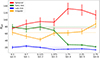 |
Fig. 5. Number counts of galaxies with different morphological types plotted as a function of redshift. Each color corresponds to a specific morphological class as indicated in the legend. The dark solid lines represent the observed counts, while the opaque solid lines represent the CSBD-corrected counts. When applying the correction the number counts for each morphological type do not change with redshift. The error bars represent the Poisson error and the contribution of cosmic variance. |
3.2.2. Results in CANDELS
This section presents the morphological fractions as a function of redshift observed in CANDELS corrected for the effect of CSBD with Method 1. We divided the CANDELS samples into seven redshift bins using the same boundaries employed for the redshifting of the galaxies of the reference sample. In each bin we measured the number counts of galaxies of a given morphological type and corrected them as explained in Sect. 3.2.1.
Figure 6 presents a plot of the observed and CSBD-corrected morphological fractions as a function of redshift for the CANDELS sample. The observed morphological fractions are shown as dashed lines, while the CSBD-corrected fractions are represented by solid lines.
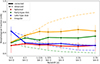 |
Fig. 6. Morphological fractions as a function of redshift in CANDELS with method 1. The observed morphological fractions are represented with dashed opaque lines, while the CSBD-corrected fractions are represented with solid lines. The influence of CSBD on the observed morphological fractions is evident, indicating a significant impact on the interpretation of the results based on visual classification. |
It can be seen that the irregular galaxies exhibit the most notable variations. At redshift z = 0.3 − 0.7, the observed and corrected fractions are nearly identical; however, at z = 2.25 − 2.75 the fraction of irregular galaxies is overestimated by a factor of ∼2.7. The observed fraction of spheroids remains relatively constant throughout the redshift range, but according to our correction method, the observed fraction is overestimated by up to 10% toward higher redshifts. The observed fraction of early-type disks increase from ∼0% at z ∼ 2.75 to about ∼20% at z ∼ 0.3, while the corrected fraction remains approximately constant at a value ∼20% at all redshifts. On the other hand, the observed fraction of late-type disks increases from ∼10% at z = 2.75 to ∼40% at z ∼ 0.3, while the corrected fraction exhibits a steep decrease from ∼60% at high redshift to nearly 40% at z ∼ 0.3. It is evident that CSBD has a significant impact on the observed morphological fractions, particularly at z > 1.0, and that this effect increases toward higher redshifts.
When splitting the CANDELS sample into star-forming and quiescent galaxies as explained in Sect. 2, we find that 19 858 galaxies fall in the first category and 3230 objects are left in the quiescent subsample. We opted not to split the reference sample into quiescent and star-forming galaxies, since there are few quiescent galaxies in the sample and the correction terms to the number counts would be statistically unreliable.
The results for star-forming and quiescent galaxies are presented in Figs. 7 and 8, respectively. The observed and corrected morphological fractions of the star-forming subsample closely resemble those of the total CANDELS sample, both qualitatively and quantitatively. This is expected since the star-forming subsample constitutes about 85.99% in CANDELS at the redshifts considered in this work. The quiescent subsample, on the other hand, exhibits distinct trends. Specifically, there is a much steeper decrease in the late-type disk class toward z ∼ 0.3, a lower irregular fraction at all redshift bins, and a sharper increase in the fraction of spheroids and early-type disks.
3.2.3. Results in the Illustris-TNG50 simulation
The morphological fractions as a function of redshift in the TNG-50 sample are plotted in Fig. 9.
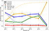 |
Fig. 9. Morphological fractions in the TNG50 sample as a function of redshift. The observed morphological fractions are represented as dashed opaque lines, while the CSBD-corrected fractions are represented as solid lines. Likewise CANDELS, the effect of CSBD on the observed morphological fractions of early- and late-type disks and irregulars is significant. |
The fraction of irregular galaxies in the observed sample decreases from approximately 95% at z = 3 to ∼20% at z = 0.5, while the corrected fraction increases from ∼30% in bin 5 to ∼50% at z = 1.5 and then decreases to ∼20% in the lowest redshift bin. For late-type disks, our findings reveal an underestimation of the observed fraction by as much as 40%. Upon correction, the fraction demonstrates a notable rise, increasing from around 5% at higher redshifts to approximately 55% at lower redshifts. Early-type disks are nearly nonexistent in the observed fraction, yet their corrected fraction spans from approximately 20% to 40%. Finally, we observe that the corrected and uncorrected fractions of spheroids are highly similar, consistently remaining at around 5% across all redshifts. Upon comparison, the observed and corrected fractions of the TNG50 sample align well with the fractions observed in the CANDELS sample.
We further divided the TNG50 sample into quiescent and star-forming galaxies based on the criterion described in Sect. 2.4. We find that star-forming galaxies comprise 76.53% of the TNG50 sample. It can be observed in Fig. 10 that the morphological fractions of star-forming galaxies closely resemble those of the entire sample, except for bin 6. In this particular bin, there is an increase in the fractions of early- and late-type disks, accompanied by a decrease in the fraction of irregular galaxies. In contrast, in Fig. 11 we see that the quiescent sample yields more complex and noisy results due to its smaller population. It can be observed that the fractions of spheroids and early-type disks increase toward lower redshifts, while irregulars and late-type disks become less frequent.
3.3. The morphological coefficients (method 2)
This section presents the investigation of the evolution of morphological fractions using the nonparametric coefficients to distinguish between different galaxy types.
3.3.1. Morphological coefficients
The use of nonparametric morphological coefficient constitutes a reliable, quantitative way of characterizing the morphology of galaxies. In particular, the Gini coefficient and the second order moment of the light distribution are indices that when combined together allow one to distinguish between bulge and disk dominated galaxies. They can be further used to select galaxies with signatures of recent mergers and low-surface brightness objects (Lotz et al. 2004, 2008; Rodriguez-Gomez et al. 2019; Sazonova et al. 2020). In this work these two coefficients are used together with the shape asymmetry As (Pawlik et al. 2016) to produce a classification with types similar to those used in Method 1.
-
The Gini coefficient (G) quantifies the inequality in the light distribution within a galaxy (Abraham et al. 2003). It is calculated by sorting the pixel fluxes in the image from lowest to highest and comparing the resulting distribution to a perfectly uniform light distribution, which is parametrized with the Lorenz curve (Florian et al. 2016). In the case of an image with n pixels each having flux Xi the Gini coefficient is defined as the mean of the absolute difference between all Xi:
 (7)
(7)where n is the number of pixels in a galaxy. G will take a value of 0 when all pixels have the same value, and will take the value 1 when all the galaxy’s flux is in one pixel. It is important to note that that the inclusion of sky pixels, and the exclusion of galaxy pixels in the calculation of G will systematically increase/decrease this index, respectively. One could consider the pixels of the galaxy as all those that exceed a threshold in surface brightness.
-
The total second order moment Mtot of the flux distribution is defined as the flux of each pixel fi multiplied by the square of the distance to the center of the galaxy, summed over all the pixels of the galaxy (Lotz et al. 2004),
![Mathematical equation: $$ \begin{aligned} M_{\rm tot}=\sum _i^nM_i=\sum _i^n f_i[(x_i-x_c)^2+({ y}_i-{ y}_c)^2], \end{aligned} $$](/articles/aa/full_html/2024/04/aa47522-23/aa47522-23-eq8.gif) (8)
(8)where xc and yc are the coordinates of the galaxy center computed by finding the pair (x, y) that minimizes Mtot. We define M20 as the normalized second-order moment of the brightest 20% of the galaxy’s flux:
 (9)
(9)where ftot is the total flux of the galaxy pixels, and fi is the flux of each individual pixel ranked in such a way that f1 is the brightest pixel. Then, M20 is a comparison between the brightness of the brightest regions to the total brightness of the galaxy, and provides a measure (values between 0 and −4.0) of how concentrated those bright regions are within the overall structure of the galaxy. Defining The 20% threshold is commonly chosen in astronomy because higher values produce unrealistic results, while lower values lead to a less discriminating statistic. Galaxies with clumpy morphology will have low values of M20.
-
The asymmetry coefficient (A) is a morphological statistic that measures the degree of rotational symmetry of a galaxy’s light distribution. It was introduced in Conselice et al. (2004) and is defined as:
 (10)
(10)where I is the galaxy flux and I180 is the flux of the galaxy in the image obtained by rotating the galaxy image by 180° about its central pixel, and B180 is the average asymmetry of the background. The shape asymmetry (As) coefficient was proposed by Pawlik et al. (2016) as a method to identify galaxies with low-surface-brightness tidal features. Unlike A, As uses segmentation maps to weight all parts of the galaxy equally and quantifies its overall level of asymmetry. The derivation of As is similar to that of A, with the difference that the segmentation maps are used instead of the science images. This approach allows for the measurement of asymmetry independently of the galaxy’s light distribution information.
We utilized the Python package STATMORPH (Rodriguez-Gomez et al. 2019) to estimate the morphological coefficients in CANDELS at z = 0.2 − 0.4. We used the PSF available in the 3D-HST repository and produced RMS maps from the weight images that were downloaded from the 3D-HST repository. To run STATMORPH we cut postage-stamp images from the original science, RMS and segmentation images and removed all the neighbors of the target object replacing them with random sky pixels from the same postage stamp.
In order to study the effects of CSBD on the measurement of the morphological coefficients, STATMORPH was run on the original and redshifted images of the reference sample. In the latter case the segmentation maps were obtained by running SExtractor (Bertin & Arnouts 1996) on the simulated image of each galaxy. Thus G, M20 and As for the redshifted galaxies were estimated within their detection areas.
3.3.2. Determination of the CSBD correction
After estimating the morphological coefficients G, M20 and As for both the original and redshifted galaxies, we obtained 268 triplets of coefficients in bin 0 (G0, M0 and A0) and 268 triplets at higher redshift bin X (GX, MX and AX). We simplify our notation by referring to M20 and As as M and A respectively.
We define the difference scalars ΔG = G0 − GX, ΔM = M0 − MX and ΔA = A0 − AX, and introduce a correction vector r = (ΔG, ΔM, ΔA), such that (G0, M0, A0) = (GX, MX, AX)+r = (GX + ΔG, MX + ΔM, AX + ΔA).
These differences are used along with the Bayes’ theorem to construct a generative model that enables the determination of the most likely values of ΔG, ΔM and ΔA for any given triplet of measured coefficients Gj, Mj and Aj in a particular redshift bin. The generative model is represented by the following probability distribution function:
 (11)
(11)
where we have assumed that:
-
Gi is linearly dependent on Mi as:
 (12)
(12) -
Mi is an independent variable.
-
Ai is an independent variable.
-
ΔG and ΔM are correlated (see Fig. 12).
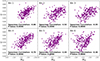 |
Fig. 12. Spearman correlation test conducted to quantify the degree of correlation between the variables ΔG and ΔM. The results indicate a significant correlation between the two variables at all redshifts. |
We assume that the likelihood term p(Gi|Mi, ΔG, ΔM) follows a normal distribution, N(μl, σl), with parameters:
 (13)
(13)
and with σl being the variance obtained by fitting a Gaussian to the distribution of the 83 measured values of ΔG. The term p(Mi|ΔM) follows a normal distribution, N(μm, σm), with parameters:
 (14)
(14)
and with σm being the variance obtained by fitting a Gaussian to the distribution of the 268 measured values of ΔM.
Similarly, the term p(Ai|ΔA) follows a normal distribution, N(μa, σa), with parameters:
 (15)
(15)
and with σa being the variance obtained by fitting a Gaussian to the distribution of the 268 measured values of ΔA.
Two important points should be noted. Firstly, the probability distribution that we seek is conditioned on the values of the unique α and β parameters for each redshift bin, as well as on the observed coefficients. Secondly, it is assumed that all terms in Eq. (11) follow a normal distribution.
3.3.3. Morphological classification in the G – M20 – As space
We note that G and M20 form a sequence which can be used to quantitatively classify galaxies. Lotz et al. (2008) introduced boundaries that divided the plane in three regions early-type (E-S0-Sa), late-type (Sb-Irr), and mergers. However, the morphological classification from Lotz et al. (2008) was designed for a low-redshift sample (0.05 < z < 0.25), and Deger et al. (2018) demonstrated its limitations at z ∼ 0.6.
To overcome this, we adopted the approach of Sazonova et al. (2020), who used Principal Component Analysis (PCA) to identify the main sequence in the G − M20 plane. The first principal component (PC1) is used to capture the highest amount of variance in the data and is aligned with the main sequence, while the second principal component (PC2) measures the distance perpendicular to it. PC1 thus provides a robust measure of the bulge strength of a galaxy and PC2 provides a way to select recently merged or low surface brightness galaxies. In order to guarantee equal weighting of both coefficients, prior to running the PCA, G and M20 were set on the same scale. This was achieved by subtracting the sample mean to each value and then dividing by the sample variance.
In Sazonova et al. (2020) galaxies were defined as having high bulge dominance if PC1 > 1 and as highly disturbed if PC2 > 1. We also use As to increase the precision of the classification. Using these three coefficients, we established the following classification criterion:
-
Spheroid: if −1 ≤ PC2 ≤ 1 and PC1 ≥ 1 and A < 0.5.
-
Early-type disk: if −1 ≤ PC2 ≤ 1 and 0 ≤ PC1 ≤ 1 and A < 0.5.
-
Late-type disk: if −1 ≤ PC2 ≤ 1 and PC1 < 0 and A < 0.5.
-
Irregular: if A > 0.5 or |PC2|> 1.
The classification criterion was tuned on the distribution of (Huertas-Company et al. 2016) morphologies in bin 0 and bin 1 within the PC1-PC2 plane. Hence, we differentiate spheroids, early-type disks, and late-type disks based on the dominance of their bulge and identify a galaxy as irregular if it exhibits a high level of asymmetry.
Our classification criterion is based on relative distances along and perpendicular to the G − M20 main sequence. The use of relative distances ensures that the boundaries need not be updated in each redshift bin to account for the intrinsic evolution of galaxies.
3.3.4. Results in CANDELS
Figure 13 plots the G − M20 planes within each redshift bin for CANDELS. When applying the CSBD correction the values of M20 decrease, while those of G increase when compared to the observed values (Table 4). As discussed earlier, the CSBD effect is characterized by a decrease in G and an increase in M20; consequently, the application of the correction derived from the probabilistic model results in a shift of the galaxies in the G − M20 plane. Figure 14 helps visualizing the shift.
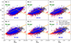 |
Fig. 13. G − M20 plane as a function of redshift in CANDELS. The estimates of the coefficients obtained from the observed data are plotted in red, while the corrected coefficients are represented in blue, and the coefficients from bin 0 are shown in gray. As a reference, the orange lines displayed on the plot indicate the boundaries defined in Lotz et al. (2008) to classify galaxies into early-type, late-type and mergers in the G − M20 plane. |
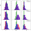 |
Fig. 14. Distributions of G (left column), M20 (middle column), and As (right column) are plotted for bin 1 (top row), bin 3 (middle row), and bin 6 (bottom row), respectively. The red histograms represent the observed values and the blue represent the CSBD-corrected values. The distribution of coefficients measured in bin 0 is plotted as a green histogram. It can be seen that in bin 1 the corrected and uncorrected distributions appear similar, suggesting that the impact of CSBD is negligible. However, in bin 6, a more pronounced difference between the observed and corrected values is evident. |
Median values of the corrected coefficients G, M20 and their median shifts for each redshift bin.
Figure 15 shows the morphological fractions of galaxies in CANDELS derived with the classification criterion described in Sect. 3.3. Solid lines refer to the fractions derived after the CSBD correction to G and M20 and dashed lines refer to those derived without applying the correction.
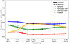 |
Fig. 15. Morphological fractions as a function of redshift in CANDELS obtained with the G − M20 − As classification. Solid lines refer to CSBD corrected values, while dashed lines refer to the observed values. It can be seen that the difference between observed and corrected fractions is small. |
It is evident that the fraction of spheroids remains relatively constant at ∼10%, experiencing a slight decrease from z ∼ 2.75 to z ∼ 1.125, followed by an increase to ∼16% around z ∼ 0.3. Early-type disks exhibit a similar pattern, starting at ∼30% in bin 6, decreasing to ∼20% in bin 2, and returning to 30% in bin 0. Late-type disks display a modest ∼5% increase in their fraction toward lower redshifts. Meanwhile, irregular galaxies maintain a fraction of about 40% up to z ∼ 1.125, subsequently decreasing to ∼15% at z ∼ 0.3.
Remarkably, unlike the results obtained with Method 1, the difference between observed and corrected morphological fractions is negligible. This aspect will be discussed in Sect. 4.
Figures 16 and 17, show the morphological fractions as a function of redshift for star-forming and quiescent galaxies, respectively.
Both the corrected and observed morphological fractions in the star-forming subsample closely resembles the fractions observed in the entire sample. As already explained, this is a result of the fact that ∼86% of galaxies in CANDELS are star-forming. On the other hand the fractions of quiescent spheroids and early-type disks decrease with redshift, while that of late-type disks undergoes a pronounced increase from ∼20% at z ∼ 0.3 to ∼60% at z ∼ 2.75. The fraction of quiescent irregular galaxies exhibits a similar trend when compared to the entire and star-forming samples. So bulge-dominated systems are predominant among quiescent galaxies at low redshift, in agreement with the scenario in which galaxies grow their bulge over time.
The reference sample used for the CSBD correction with Method 1 contains only 258 galaxies, and when splitting in bins of stellar mass, the number of galaxies in each bin would be too small to derive a statistically significant correction. For this reason we did not investigate the effect of CSBD as a function of stellar mass when we used Method 1. However, since we can measure G and M20 for each galaxy, this analysis becomes possible with Method 2. Figures 18–20 show the morphological fractions plotted as a function of stellar mass for each morphological type defined in the G − M20 − As plane.
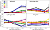 |
Fig. 18. Morphological fractions obtained with method 2 plotted as a function of stellar mass in CANDELS. Each panel represents a morphological type, and the values in each redshift bin are plotted in the same color. The dashed lines correspond to the observed, uncorrected fractions. |
It can be seen from Fig. 18 that the fraction of spheroids is approximately constant with mass down to z ∼ 0.7. Below this redshift the fraction present a noticeable increase with stellar mass which suggests that elliptical galaxies dominate the morphological mix at high stellar masses at low redshifts. Interestingly, this behavior is also apparent in the star-forming subsample (Fig. 19), while in the quiescent subsample (Fig. 20) it starts earlier, at z ∼ 1.75. The increase with mass of the fraction of quiescent spheroids is steeper for quiescent galaxies than for star-forming galaxies. The rise in the fraction of high-mass spheroids implies tha the spheroid population becomes enriched with medium-high mass galaxies with time. This observation suggests that spheroids undergo an increase in stellar mass, likely through dry mergers as discussed in Lidman et al. (2013), Ownsworth et al. (2014), or Rodriguez-Gomez et al. 2016.
The fraction of early-type disks does not present significant variations with redshift. At z ∼ 0.3 the fraction reaches values of 0.4–0.6, exhibiting two maxima at 1010 and 1011 M⊙. While the first maximum is statistically significant, the second is consistent within the errors with the values of the fraction at higher redshifts. The fraction of early-type disks in star-forming galaxies follows a trend similar to the overall CANDELS sample. Quiescent galaxies, on the other end, show a different trend, in which the fraction of low-mass early-type disks becomes higher at z < 0.7. It should be stressed, however, that the values of the fractions in this subsample are all consistent within the errors; therefore, any conclusion on their trends with redshift should be drawn with caution.
The late-type disk fraction mirrors the trend observed in spheroids: at high redshifts (z > 1), the fractions of high-mass late-type disks range between 0.4 and 0.6, while at z < 0.7 they are less than 0.2. Interestingly, the fraction of low-mass late-type disks (< 1010 M⊙) reaches 0.5–0.6. This behavior is also observable in star-forming galaxies. Similarly, the fractions of quiescent late-type disks exhibit a slightly increasing trend with stellar mass at z > 1.0 which then turns into a decreasing trend at z < 0.7. However, the errors at < 1010 and > 1010.5 M⊙ are large, and the difference between the fractions at different redshifts are not significant. The decline in the fraction of irregular galaxies shows no dependence on stellar mass.
Figure 21 displays the median and the 1σ widths of the distributions of G, M20, AS, and half-light radius as a function of redshift. It can be observed that, in general, as the redshift increases, G and the half-light radius decrease and, as a result of that, galaxies may appear fainter and smaller. Conversely, M20 and the shape-asymmetry increase, suggesting a clumpier and more asymmetric appearance for high redshift objects.
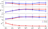 |
Fig. 21. Median and 1σ widths of the distributions of the observed (red) G, M20, As, and half-light radius (Re) are displayed from top to bottom in each panel. The median of the corrected G, M20 and As values are shown as blue lines. |
Although these results may explain why visual classifiers tend to assign irregular morphologies to galaxies at high redshift, the observed and corrected median values of G, M20 and As are consistent within the widths of the distributions, indicating that the difference is not statistically significant. Further elaboration on this topic will be provided in the discussion.
3.3.5. Results in the Illustris-TNG50 simulation
The morphological coefficients for the TNG50 simulated galaxies were derived running STATMORPH on the HST-like images published in Snyder et al. (2017).
As shown in Fig. 22, the fractions of all morphological classes undergo minimal variations across the examined redshift range. Nonetheless, it is remarkable that observed and corrected fractions exhibit differences in this sample. The observed fractions of spheroids and irregulars are overestimated by approximately ∼5% and ∼20%, respectively. The observed and corrected fractions of early-type disks are quite similar, whereas the fraction of late-type disks is underestimated by up to ∼30%. We also looked at the trends of the star-forming and quiescent subsamples; however, we find inconclusive results and a large scatter in both subsamples.
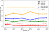 |
Fig. 22. Morphological fractions as a function of redshift in TNG50 estimated with method 2. The observed and corrected fractions are shown in dashed lines and solid lines, respectively. |
The morphological fractions as a function of stellar mass (Fig. 23) reveal no notable evolutionary trend for spheroids: there is a higher fraction at M* > 1010 M⊙ in bin 1, but the values are consistent with those of the fractions at higher redshift. Early-type disks tend to be more abundant at > 1011 M⊙ in bin 1, although their values are again consistent with those at higher redshifts. Late-type disks, on the other hand, exhibit an increase in the fraction with mass in bin 6 and bin 3, while there is no significant trend at lower redshifts. Irregular galaxies do not display a distinct trend, but their corrected fractions are consistently lower than the observed ones.
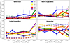 |
Fig. 23. Morphological fractions estimated with method 2 as a function of stellar mass in TNG50. Each panel represents a morphological type, and the values in each redshift bin are plotted in the same color. The dashed lines correspond to the observed, uncorrected fractions. |
4. Discussion
4.1. The effects of cosmological surface brightness dimming on morphological classifications
The comparison between the observed and CSBD-corrected morphological fractions in CANDELS and TNG50 shows that CSBD introduces a significant bias in the visual morphological classification of galaxies. Figure 24 illustrates the difference between observed and corrected morphological fractions in the CANDELS sample. The fractions of irregular and spheroidal galaxies are overestimated: spheroids are overestimated by approximately 10% at all redshifts, while irregular galaxies are greatly overestimated, reaching up to 50% at high redshifts and gradually declining to nearly 0% in the lowest redshift bin. On the other hand, the fractions of both early-type and late-type disks are underestimated by up to 10% and 50%, respectively. The overestimation and underestimation of these fractions becomes significant at z ≥ 1, in agreement with what would be expected by the (1 + z)−4 law.
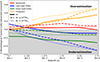 |
Fig. 24. Over- and underestimation of the observed morphological fractions in CANDELS as a function of redshift. Dotted, dashed and solid lines represent the low-stellar mass sample (M* < 1010 M⊙), high-stellar mass sample (M* ≥ 1010 M⊙) and the entire sample, respectively. The y-axis represents the difference between the observed and corrected fractions. So all the values within the light-gray region correspond to underestimations of the morphological fractions, while the white area indicates the overestimation. Notably, the differences between the observed and corrected fractions increase with redshift, with the exception of the spheroid class. |
We also find that for a given redshift bin, high-stellar mass (M* ≥ 1010 M⊙) spheroids and low-stellar mass (M* < 1010 M⊙) irregular galaxies tend to be more overestimated with respect to what happens if we consider the entire CANDELS sample. High-stellar mass early- and late-type disks seem to be less underestimated than low-stellar mass disks.
One of the remarkable results of this paper is that the effect of CSBD is significant in visual classifications but negligible for the classification based on the G, M20 and As coefficients. This means that a low-z galaxy and an artificially redshifted version of it may appear different to the eye and still have similar values of the two morphological coefficients.
When artificially degrading a galaxy image, we modify its surface brightness and its pixel scale. G is sensitive to the cumulative distribution of the flux of the galaxy pixels, while M20 is sensitive to the width of the flux distribution. The degradation factor of (1 + z)−4 can be understood as a simple multiplication of the pixels flux values by a constant, which should not significantly affect the shape of the flux distribution.
However, after redshifting, the values of G and M20 may be affected when the pixel flux falls below the source detection threshold, that is, lower than the sky background. The number of pixels that fall below the sky value increases with the redshift of the simulation and, when it becomes high enough, the detected part of the galaxy may have a different shape from the original. In particular, the values of the faintest pixels may differ enough to affect the measurements of the coefficients.
Figure 25 shows the changes in visual appearance and the estimated morphological coefficients between bin 0 (z ∼ 0.3) and bin 6 (z ∼ 2.75) for a spheroid, late-type disk and an irregular galaxy from the reference sample. One can notice that despite the evident change in visual appearance between the original and the redshifted versions, (e.g., the spiral arms in the late-type disk disappear completely bin 6) there is only a small change in the morphological coefficients. This suggests that while the changes in morphological coefficients resulting from the change in pixel scale and CSBD are not significant, the human eye is unable to distinguish small flux differences between the object and the sky. This explains why G and M20 do not change between the original and simulated images in the reference sample despite the difference perceived by the human eye.
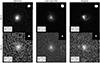 |
Fig. 25. Three example images of artificially redshifted galaxies. Top row: images of three galaxies from the reference sample at bin 0, a spheroid, an early-type disk, and an irregular. Bottom row: redshifted versions of the galaxies in bin 6 (z ∼ 2.75). Each panel shows the morphological coefficients estimated for a galaxy in the bottom left corner and its segmentation image in the top right corner. Despite the evident change in visual appearance, the variations in the morphological coefficients are small. |
On the other hand, As exhibits the highest variation since the segmentation image is used to estimate it. It is indeed important to remind that SExtractor is run on every simulated image; therefore, in each redshift bin there is a segmentation map for a given galaxy.
The analysis of Fig. 21 reveals that galaxies at high redshifts display a combination of characteristics: higher M20 and asymmetry, smaller effective radii, and smaller G. This combination suggests that some of these galaxies may appear smaller and fainter when compared to galaxies at low redshifts, resembling low-mass elliptical galaxies. Other galaxies may have lower values of G and higher shape asymmetry due to the presence of substructures (such as disordered spiral arms and tidal tails) or a stronger confusion between galaxy pixels and background pixels, and thus they may have a less concentrated light distribution, resembling an irregular galaxy. However, it is important to note that the values of both the observed and corrected median values of G and M20 are consistent at all redshifts. Therefore, the slight changes in the median values of these coefficients are not statistically significant at z ≤ 2.25.
So, the CSBD results in a significant change in the aspect of galaxies, which appear either rounder and fainter or asymmetric and fainter, but a small change in the morphological coefficients. One may say that the human eye tends to “exaggerate” the morphological differences between the low-z galaxies and their redshifted counterparts.
Therefore, based on the information provided by Figs. 4, 24 and 21, we propose two confusion channels to explain these results. Regardless of their true morphology, galaxies tend to be visually misclassified as spheroids or irregulars. Galaxies can be mistaken for spheroids because the observed surface brightness of extended structural features, such as the disk, may fall below the sky level and consequently not be discerned during the visual inspection. This leads an observer to classify a galaxy as a spheroid. On the other hand, galaxies could be misclassified as irregular galaxies because they appear fainter and asymmetric.
4.2. Morphological fractions
Our findings on the morphological fractions in CANDELS with the visual-classification method (Fig. 6) suggest that galaxies do experience morphological transformations since z = 3. The main evolution found is that the (corrected) fraction of late-type disks decreases between z ∼ 2.75 and z ∼ 0.3, while that of irregulars increases in the same redshift range. The fraction of spheroids and early-type disks increase toward z ∼ 0.3.
When splitting the CANDELS sample into star-forming and quiescent galaxies, it can be seen that star-forming galaxies have a behavior similar to the entire sample. However, while the fractions of star-forming spheroids and early-type disks are only mildly increasing toward low redshifts, the fractions of their quiescent counterparts exhibit a ∼20% increase. Interestingly, the fractions of both star-forming and quiescent late-type disks decrease toward lower redshifts, while the fraction of star-forming irregulars is approximately constant and that of quiescent irregulars decreases toward low redshift. These results suggest that star-forming late-type galaxies quench star formation and then transform into early-type disks. The increase in the fraction of elliptical galaxies at low redshifts, which is more pronounced at high stellar mass at z < 0.7 supports a scenario in which these galaxies originate mostly from mergers. It can be seen that the fraction of star-forming irregulars maintains approximately constant with redshift. This suggests that part of the star-forming late-type disks may transform into irregulars if they are undergoing a process of merger with other galaxies.
The results obtained with Method 2 (Fig. 15) indicate a distinct evolutionary pattern from Method 1. The fractions of spheroids, early- and late-type disks show a slight increase down to z ∼ 0.3, while the fraction of irregular galaxies increases up to z ∼ 1.125 and then declines. Star-forming galaxies closely reproduce these trends with a slightly more pronounced increase in the fraction of late-type disks. Quiescent galaxies, on the other hand, exhibit trends more similar to those found with Method 1, but with a 20% higher fraction of irregular galaxies. These results support a scenario in which star-forming irregular galaxies evolve into spheroids, and late-type disks transform into either non-star-forming spheroids or early-type disks.
Several studies have been conducted to explore the evolutionary paths of galaxies with different morphologies. Conselice et al. (2005) performed visual classifications of H-band HST-images of galaxies in the Hubble Deep North and South Fields up to z ∼ 3. Their findings revealed a dominant fraction of peculiar galaxies, those galaxies characterized by perturbations or indication of merger activity (Abraham et al. 1996), at redshifts z > 2. However, this fraction showed a steep decline, accompanied by an increase in the fractions of elliptical and spiral galaxies. Whitney et al. (2021) observed a similar trend in CANDELS up to z ∼ 3, utilizing visual classifications from Kartaltepe et al. (2015). They observed a power-law increase in the fractions of spheroids and disks from approximately 25% at z = 2.5 to over 45% and 35 − 40% at z = 0.5, respectively, while the fraction of peculiar galaxies exhibited a linear decrease from approximately 45% at z = 3.0 to approximately 15% at z = 0.5.
The results of Conselice et al. (2005) and Whitney et al. (2021) exhibit significant discrepancies when compared to ours. However, as previously mentioned, visual classifications are strongly influenced by the effects of CSBD and limitations in human visual perception resulting from the loss of information, and thus a direct comparison must be done carefully.
The forthcoming generation of high-redshift surveys, such as those that are being or will be carried out with JWST, ELT and the Vera Rubin Telescope, present an opportunity to expand upon the present study and effectively assess the impact of CSBD at lower and higher redshifts. These surveys will benefit from enhanced resolution and depth (for example, LSST will be very deep after 10 years of observations), enabling more accurate and comprehensive quantitative as well as qualitative morphological classifications. Additionally, they will provide an initial glimpse into the morphology of high-redshift galaxies. Therefore, these surveys hold great promise in advancing our understanding of the subject.
Recent investigations conducted on images from JWST have already shed light on the morphological fractions of field galaxies at z > 3. For example, Jacobs et al. (2023) employed visual classifications on a sample of field galaxies ranging from z = 0.8 to z = 5.4. They found that for galaxies with stellar masses above 109.5 M⊙ there is a steeply decreasing trend from ∼80% at z ∼ 5 to ∼20% at z < 2.55 for peculiar galaxies, a mostly ∼20% constant fraction of spheroids at all redshifts, and an increasing fraction of early-type (disk+spheroid) and late-type disks. These findings align with recent CNN-morphological measurements derived from JWST images in Huertas-Company et al. (2023), who revealed a substantial fraction of regular galaxies (comprising disks and bulges) at high redshifts within the higher mass ranges (10.5 < log(M*/M⊙) < 11.5). In particular, they found the same decrease of the irregular galaxy fraction from z ∼ 5 to z ∼ 2, a sort-of constant fraction at ∼20% for spheroids and late-type disks, and an increase of the early-type disk fraction, from ∼20% at z ∼ 5 to ∼40% at z ∼ 1. Ferreira et al. (2022) derived morphological coefficient-estimated morphological fractions with JWST images for the SMACS-0723 galaxy cluster, finding a decreasing trend for the fraction of spheroids, an increasing peculiar fraction and a constant disk fraction from z ∼ 5 to z ∼ 2. The fact that disk and spheroids are more common at z > 2, compared to what is seen with HST measurements, challenge the build-up timescale of the of the Hubble sequence.
Jacobs et al. (2023) have also found that galaxies at high redshift exhibit higher levels of asymmetry in comparison to their local counterparts. The increased asymmetry observed in these high-z galaxies may be attributed to a greater frequency of ongoing interactions and mergers, which in turn contribute to morphological transformations. This aligns with the findings of Ferreira et al. (2022), who reported a rise in the proportion of post-merger galaxies within the redshift range 0.5 < z < 2.5, ranging from approximately 20% to 25% depending on the mass of the galaxies. This work shows, however, that the higher asymmetry observed in galaxies at higher redshifts could be partially attributed to CSBD. Therefore, it is important to conduct a thorough investigation into the effects of CSBD on asymmetry in order to validate the true nature of the enhanced asymmetry in high-redshift galaxies.
The results from these studies align, to some extent, with our results. However, some discrepancy is expected as these studies do not account for the effect of CSBD. Considering that the CSBD follows a (1 + z)−4 law, it is expected that the CSBD effect will be even more relevant in the visual classification of galaxies at z > 3. Consequently, the fractions of spiral galaxies could be even higher, while the fractions of elliptical galaxies may be lower than what has been observed. Given that we have demonstrated the impact of CSBD at lower redshifts, it is crucial to incorporate these corrections when analyzing galaxies at z > 3. The high-redshift visual morphological fractions measured in the studies previously mentioned show a decrease in peculiar galaxies, which should be overestimated according to our conclusions. In the same manner, the increasing fraction of disks should be underestimated.
Figure 26 shows that there is a large scatter between the results on morphological fraction from different studies. The observed fractions of spheroids estimated with Method I (dark red) are consistent with the results from Jacobs et al. (2023) and Margalef-Bentabol et al. (2022), while the fractions of late-type disks agree better with the measurements of Mortlock et al. (2013), Margalef-Bentabol et al. (2022) and in the highest redshift bins with those of Conselice et al. (2005). The fractions of early-type disks, on the other hand, are lower than those reported in the literature, while the fractions of irregular galaxies agree best with the results of Mortlock et al. (2013). When looking at the CSBD corrected morphology, it can be seen that the fractions of spheroids and early-type disks are systematically lower than in other studies. The fraction of late-type disks agrees best with the results of Huertas-Company et al. (2023), Whitney et al. (2021) and Margalef-Bentabol et al. (2022), while the fraction of irregular galaxies agrees best with the results of Whitney et al. (2021) and Conselice et al. (2005). When compared with the results reported in the literature, the fraction of late-type disks in this work is above the average.
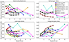 |
Fig. 26. Morphological fractions as a function of redshift from published works. The plot includes Conselice et al. (2005; blue), Lotz et al. (2004; red), Mortlock et al. (2013; green), Whitney et al. (2021; purple), Margalef-Bentabol et al. (2022; yellow), Ferreira et al. (2022; orange), Huertas-Company et al. (2023; pink), and Jacobs et al. (2023; turquoise). The observed morphological fractions in this study are plotted in dark red, and the corrected morphological fractions obtained with Method 1 and Method 2 are plotted in gray and black, respectively. |
It is important to stress that the criteria and methods used for the morphological classification in each work are different; therefore, any comparison with the literature. This is surely a source of discrepancy between the results of the present work and those published in the literature. For instance, previous studies considered ellipticals and lenticulars as spheroids, whereas we classify S0 galaxies as early-type disks and treat ellipticals as a distinct class. Furthermore, peculiar galaxies, although seemingly irregular at first order, are a different class from irregular galaxies. In general there are two main sources of disagreement with the literature: i) the broader and fundamentally different spheroids/disks/peculiar classification scheme employed in these studies, and/or ii) the omission of explicit considerations for the effects of CSBD in the morphological measurements.
Among all the results presented for comparison in Fig. 26 only the measurements of Mortlock et al. (2013) and Margalef-Bentabol et al. (2022) were corrected for CSBD. The latter study found that the corrected fraction of spirals increases by ∼15% when going from z = 2.5 to z = 0.5, which agrees with our statement that the fraction of disk galaxies at high redshift is underestimated. However, our results diverge from those reported in these two studies because of the different definitions adopted for the morphological types.
With the impact of the CSBD being more significant in the visual classification than in the classification based on morphological coefficients, we have chosen to rely on the results obtained from the second classification method for our analysis. Quantitative classification proves to be more robust and reliable compared to visual classification, particularly when dealing with “intermediate classes” such as early-type disks. Therefore, we expect that Method 2 is able to capture subtle variations in light distribution and thus accurately characterize the morphology of galaxies.
4.2.1. Morphological fractions as a function of stellar mass
Huertas-Company et al. (2023) found that spheroids at z > 1 have stellar masses exceeding 1010 M⊙. However, lower-mass spheroids become more prevalent at z < 1. Early-type disks progressively gain mass as one approaches the present epoch, reaching a fraction of approximately 50% in the highest mass bin at z = 0 − 1. Late-type disks, on the other hand, exhibit an increase in their number in the intermediate mass range, spanning from 109 to 1010 solar masses toward z = 0. Finally, irregular galaxies have a higher fraction at low masses, with a fraction close to 100% between z = 3 and z = 6. Nonetheless, this fraction declines to approximately 70% for redshifts below 1. Martin et al. (2020) finds a similar trend, with spheroids dominating the high-mass end at high redshift (z ∼ 0.9), and the fraction of early-type disks (S0-Sa) being higher at high masses at z = 0.
Interestingly, Varma et al. (2022) found similar trends for star-forming and quiescent spheroids and early-type disks. However, they found that irregulars and late-type disks have higher fractions regardless of their star formation regime. In particular, they find that the fraction of late-type disks becomes higher at high masses and that of irregulars increases at low stellar masses at z = 0.
We observe distinct evolutionary trends with stellar mass. Specifically, at z < 0.7 spheroids are more abundant at high stellar masses, while early- and late-type disks are more common at low stellar masses. Irregular galaxies do not exhibit any discernible trend with stellar mass. The star-forming subsample closely mirrors these trends, while the quiescent subsample exhibits similar trends but with greater strength. It is essential to emphasize that our sample is limited in mass, so this outcome is not merely a result of survey depth.
Our primary findings generally align with these studies: early- and late-type disks with low stellar mass show an increased fraction toward lower redshifts, while the fraction of high-mass spheroids rises toward lower redshifts. This alignment is consistent with the scenario of bulge growth in galaxies.
4.3. Morphological fractions in simulations
Simulations provide another useful source of comparison. Some studies, such as Huertas-Company et al. (2019) and Varma et al. (2022), show that the fractions of spheroids, early-type and late-type disks increase with stellar mass at lower redshift, while irregulars galaxies constitute the majority of the galaxy population at z > 1.5 with a fraction of up to ∼80%, decreasing to ∼20% at z = 0.5.
From Varma et al. (2022), it can be seen that the morphological fractions of star-forming galaxies in TNG50 have a very similar trend to those of the entire sample, while quiescent galaxies display a more complex behavior. At first order, we can distinguish that early-type disks and spheroids become more prominent in lower mass bins toward lower redshifts, and the same happens for late-type disks.
We find that there are no significant trends with mass in TNG50 aside from a mild increase in the fraction of spheroids and early-type disks at intermediate and high masses at z ∼ 0.5 and an increase in the fraction of late-type disks with mass at z > 2. Irregular galaxies do not show a distinct trend with stellar mass, aside from statistical fluctuations. However, the corrected fraction is approximately 10 − 20% lower than the observed fractions.
The morphological fractions in the TNG50 sample obtained with Method 1 exhibit a closer qualitative resemblance to previous findings from other studies compared to those obtained with Method 2. This observation suggests that, while galaxies in TNG50 successfully capture the visual appearance of real galaxies, the simulation might fall short in replicating the light distribution. Consequently, this discrepancy could lead to the derivation of morphological coefficients that differ from their real counterparts.
Making a direct and quantitative comparison between our results and those of previous studies is challenging. The diversity of methods used to characterize the morphology of galaxies and the limited consideration of CSBD in previous studies highlight the need for careful interpretation when comparing results.
We further emphasize that the boundaries that we use to distinguish morphological types in the G − M20 − As space are conservative, and we might be only capturing a subset of galaxies of any morphological type. Trying different definitions for morphological classes is beyond the scope of this work, whose principal aim is to determine the way in which CSBD affects the determination of the morphology of distant galaxies.
4.4. Morphological transformations and star formation quenching
Our results support the notion that late-type disk galaxies terminate star formation and undergo morphological transformation. High-mass late-type disks terminate to form stars earlier than their low-mass counterparts.
We propose two channels for morphological evolution and quenching. The first channel involves galaxy mergers. As shown in Marchesini et al. (2014), the likely progenitors of massive quiescent galaxies in the local Universe are massive late-type disks at z ∼ 3. These galaxies undergo a merger event and predominantly transform into massive spheroids without star formation. In this case, the quenching can occur either before or during the merger event. Secular evolution is less plausible in this channel. Our results indicate that late-type disks that cease star formation do not persist as disks but transform into spheroids, especially at high masses. To achieve this morphological transformation and mass increase in late-type disks, a merger event is required, as secular evolution alone is insufficient.
The second channel involves secular evolution. Low-mass quiescent galaxies also originate from late-type disks, but their mass does not increase because they do not undergo mergers. This explains why they populate the low and intermediate mass regions. The quiescent late-type disks may lose their spiral arms due to secular evolution or grow their bulge through minor dry merger, transforming into early-type disks. Quiescent early-type disks may later undergo major merger and enrich the population of massive elliptical galaxies observed at z < 0.7.
Minor and major mergers are good candidates to explain both morphological transformation paths for late-type disks. Dry major mergers can completely disrupt the disk of a late-type galaxy, transforming the galaxy into a spheroid, while dry minor mergers can smooth out the disk, transforming the galaxy into an early-type disk.
Previous studies such as Bluck et al. (2022) have examined the role of bulge growth in the process of star formation quenching. They found that the stellar mass of the bulge is the primary predictive parameter for quenching, surpassing the significance of other quantities such as the disk mass, the total stellar mass, and the bulge-to-total ratio (B/T). Consequently, it can be inferred that the quenching of star formation is driven by mechanisms that take place in the bulge, such as AGN. Extensive analyses in the literature have focused on the process of bulge-growth through mergers (e.g., Hopkins et al. 2010; Brooks & Christensen 2016). It has been found that galaxy-satellite collisions increase the Sérsic index n and the bulge mass proportionally to the satellite mass Aguerri et al. (2001).
Notably, the same is seen in simulations. Huertas-Company et al. (2019) conducted a study utilizing the IllustrisTNG simulation and demonstrated that the majority of massive galaxies exhibit a higher proportion of ex-situ stellar mass. Given the consistency of our findings with Method 1 with the results obtained from the TNG50 simulation, it can be inferred that the mechanisms governing galaxy formation, evolution, and morphological transformations as implemented in IllustrisTNG are capable of predicting observing results.
Another bulge-growth explanatory mechanism that has been proposed is the radio-mode AGN feedback. In this process, the accretion of material onto a supermassive black hole (SMBH) generates powerful outflows of energy. These outflows expel or heat the surrounding gas, effectively suppressing star formation (Carilli & Walter 2013).
Recent determinations of the growth rate of massive black holes taking into account the cosmic SFR density suggest that the peak of black hole accretion is consistent with the peak of star formation, indicating a close relationship between star formation quenching and black hole growth (Madau & Dickinson 2014). Varma et al. (2022) conducted a study using the TNG50 simulation and discovered a link between supermassive black hole (SMBH) activity and the morphological transformation of massive galaxies. They found that when the SMBH enters a low-accretion state, known as the kinetic-feedback mode, gas is rapidly depleted, increasing the observed central mass density of the galaxy and eventually resulting in quenching. Another study by Koutsouridou & Cattaneo (2022) supports this scenario, stating that morphological transformation plays a crucial role in quenching. They explain that during galaxy mergers, the transformation of disks into bulges occurs, which simultaneously feeds the SMBH. Star-forming galaxies, with a SMBH in quasar-mode, experience an increase in SMBH mass through mergers until a radio mode nuclear activity is reached. This nuclear activity is capable of heating the surrounding gas, preventing gas cooling and thus resulting in the quenching of star formation. Consequently, galaxies undergo an inside-out quenching process (e.g., Genel et al. 2014; Tacchella et al. 2015; Bluck et al. 2020).
Our results support the notion that high-redshift late-type disks undergo mergers, increasing their bulge mass and quenching star formation. Alternatively, disk galaxies may undergo secular evolution, with mass being gradually accreted by the bulge from the disk.
An important aspect to consider is the presence of star-forming spheroids and quiescent disks within both the CANDELS and TNG50 samples. This observation aligns with the findings of Brennan et al. (2015), who investigated the assembly of galaxies using the specific SFR versus Sérsic index (n) plane. They classified galaxies into four populations: star-forming/quiescent disks and star-forming/quiescent spheroids. Their analysis demonstrated that a model incorporating bulge growth through both disk instabilities and mergers provides a better fit to the observed distribution of these four populations within the CANDELS dataset.
Furthermore, de Sá-Freitas et al. (2022) discovered evidence supporting different formation processes for quenched disk-like galaxies and quenched spheroids. Quenched disk-like galaxies are more likely undergoing secular processes, such as internal dynamical instabilities, while quenched spheroids have likely experienced more violent interactions, including major or minor mergers, which may have influenced their star formation histories. Additionally, the presence of blue cloud ellipticals (Schawinski et al. 2014), which are predominantly found in low-density environments (Bamford et al. 2009; Dhiwar et al. 2023), suggests the occurrence of post-merger objects with residual star formation or post-rejuvenation processes that have led to their current properties.
In line with these findings, Lu et al. (2021) discovered a decreasing fraction of AGN observed in quiescent late-type galaxies over time, indicating the role of AGN feedback in maintaining quiescence in these systems. Conversely, the high fraction of AGN observed in star-forming elliptical galaxies implies the involvement of positive AGN feedback. In this scenario, AGN-driven outflows compress the gas, leading to its collapse and subsequent formation of new stars, thereby triggering star formation (Cresci & Maiolino 2018; Nesvadba et al. 2020).
It is also important in this context to assess the role of the local environment, since the field comprises a variety of large-scale structures encompassing groups, filaments and voids. The environment affects the quenching of star formation since galaxies may interact with their neighbors.
Several studies have investigated the factors influencing quenching timescales, stellar mass, and the role of the environment in star formation quenching and morphological transformations. Wetzel et al. (2013) and Hahn et al. (2017) focused on satellite and central galaxies in clusters, respectively, and found that more massive galaxies exhibit shorter quenching timescales. Walters et al. (2022) demonstrated that quenched galaxies tend to have higher stellar and halo masses, as well as larger effective radii. Gu et al. (2021) highlighted the importance of stellar mass as a dominant variable in quenching massive galaxies at high redshifts (z > 1), whereas environmental quenching is more effective for low-mass galaxies at lower redshifts (z < 1).
Lu et al. (2021) reported distinct mass distributions and local environment density distributions for quiescent and star-forming galaxies at z < 1.5 for a given morphological type. They also found that, for a given star formation regime, bulge- and disk-dominated galaxies have different mass distributions but similar local density distributions. These findings suggest that stellar mass plays a crucial role in quenching and morphological transformations at high redshifts, while local galaxy density primarily affects quenching but has a lesser impact on morphological transformations. This indicates that galaxy morphology is more closely related with star formation than with the environment at high redshifts. Nonetheless, as time progresses, the influence of galaxy mass on its morphology becomes less prominent as environmental quenching gains more significance Gu et al. (2021).
5. Summary and conclusions
We present estimations of the morphological fractions of field galaxies at 0.2 < z < 3.0 from the CANDELS survey. We conducted a detailed analysis of the effects of CSBD on the morphological classification and on the measurements of morphological coefficients. For this purpose, we selected a sample of 268 galaxies from all five CANDELS fields at redshift 0.2 ≤ z < 0.4 and simulated them at higher redshifts, accounting for CSBD, resolution, and the S/N. We used two characterizations of galaxy morphology, namely the visual classification and the G − M20 − As space.
We studied the morphological fractions in CANDELS and compared our results with those obtained on mock images built from the TNG50 simulation. We investigated the morphological fractions as a function of stellar mass. Finally, we studied the change in redshift of the morphological fractions for the entire galaxy population and for the subsamples of star-forming and quiescent galaxies. Our main findings are the following:
-
CSBD is a significant source of bias in visual classification. The confusion between morphological types manifests itself in the fact that at high redshifts the numbers of spheroidal and irregular galaxies are overestimated by 10% and 50%, respectively, while the numbers of early- and late-type disks are underestimated by up to 50%. Thus, human classifiers and, likely, machine learning and deep learning models trained on visually labeled samples, tend to classify distant galaxies more easily as spheroids or irregulars than as disk-dominated. The magnitude of this effect becomes significant at z ∼ 1.125 and increases at higher redshifts.
-
There are two primary confusion channels that result from CSBD on visual classification. The first channel comprises the spheroid versus disk confusion, which consists in the fact that the lowest surface brightness features in galaxies, such as the disks, may fall below the sky level, giving the appearance of a spheroid to an actual disk galaxy. The second channel consists in the irregular versus regular confusion, which stems from the increase in M20 and As and the decrease in G, which cause a galaxy, regardless of its actual morphology, to appear irregular to a human classifier or to be classified as such by an algorithm trained on visual labels.
-
Higher-redshift galaxies tend to exhibit lower values of G and half-light radius, and higher values of M20 and As, indicating that distant galaxies appear smaller, fainter, clumpier, and more asymmetric than their low-redshift counterparts. We find that CSBD does not have a significant impact on the estimation of the morphological coefficients G, M20, and As at z < 2.25. We find that the dimming of galaxies, the dropout of pixels with fluxes below the source detection threshold, and the change of pixel scale do not significantly affect the distribution of the pixel flux and the flux distribution width. Therefore, morphological coefficients are able to trace the light distribution of a galaxy more reliably than the human eye for low-surface brightness objects. Nevertheless, notable changes start to emerge at z > 2.25, highlighting the need for further investigation into morphological coefficients at higher redshifts.
-
Morphological fractions derived with the G − M20 − As space classification indicate that, except for irregular galaxies, the morphological fractions are consistent with a constant trend with redshift.
-
The morphological fractions of the star-forming galaxies in CANDELS exhibit trends with redshift that are similar to those observed in the entire sample. We attribute this effect to the fact that ∼86% of the galaxies in the survey are star-forming. However, when studying the morphological fractions in quiescent galaxies, we observed a decline in the fraction of late-type disks mirrored by an increasing fraction of early-type disks and spheroids toward z ∼ 0.3.
-
When examining the morphological fractions as a function of stellar mass, we found that the spheroids populate the highest stellar mass bins (M* > 1010 M⊙) at low redshifts, while early- and late-type disks populate the lower-mass bins. The same trends were found for both star-forming and quiescent galaxies. The fraction of irregular galaxies does not depend on stellar mass at all redshifts.
-
High-redshift massive late-type disks undergo a transformation into quiescent spheroids and/or early-type disks. We propose two quenching channels, namely merger and secular evolution. Late-type disks could undergo one or several merger events, losing their disk and transforming into a spheroid while gaining stellar mass. The merger event may increase bulge mass, a well-known quenching driver. Alternatively, late-type disks may undergo secular evolution or experience quenching through processes such as AGN feedback or black-hole feedback.
-
The results obtained from the CANDELS sample using method 1 partially align with those observed in TNG50, indicating a degree of reliability in the predictions of this simulation. However, notable discrepancies emerge between the results from the CANDELS and TNG50 samples when applying method 2. This suggests that simulated galaxies may not reproduce the light distributions of real galaxies accurately.
We do find discrepancies between our results and the morphological fractions as a function of redshift and stellar mass measured in previous studies. We argue that these discrepancies are mainly due to the fact that most of the morphological fractions in the literature do not account for the effect of CSBD, which we have proven to be a significant source of bias for visual classifications at z > 1. Furthermore, the classification criterion that we adopted to define the classes in the G − M20 − As space uses arbitrary boundaries that need to be tuned to have a better match to visual morphology. We are currently working on refining the classification boundaries in order to avoid over- and underestimation of the number of galaxies of a given morphological class. The next step in our research is the construction of an empirical model for the physical interpretation of the results and trends reported in this work.
In order to achieve statistical significance in our findings, our aim is to conduct these experiments using a larger reference sample. However, the inclusion of a larger sample leads to the use of automatic techniques. In the present study, the reference sample comprised 268 galaxies, which meant that a total of 1608 galaxies had to be classified by two people. The classification of a larger sample will be more viable by training a machine or deep learning model.
We finally note that the present work has been developed within a collaboration that is aimed at studying the structural evolution in different cosmic large-scale structures. A work on the morphological evolution of galaxies in a sample of clusters at z = 0.2 − 0.9 from the Cluster Lensing and Supernova Survey with Hubble (CLASH, Postman et al. 2012) is currently ongoing (Cerulo et al. in prep.). By comparing the results obtained in clusters with those presented here, we will be able to draw a picture of the structural changes of galaxies in different environments.
The United Kingdom Infra-Red Telescope.
Available http://arcoirix.cab.inta-csic.es/Rainbownavigatorpublic/.
Available https://archive.stsci.edu/prepds/3d-hst/.
The Petrosian ellipse is an ellipse that encloses a fixed fraction of the total flux of a galaxy, regardless of its shape. The Petrosian flux is the amount of light that falls within the Petrosian ellipse.
Diego Salvador and Pierluigi Cerulo.
Acknowledgments
This work has made use of the Rainbow Cosmological Surveys Database, which is operated by the Centro de Astrobiología (CAB), CSIC-INTA, partnered with the University of California Observatories at Santa Cruz (UCO/Lick,UCSC). This work is based on observations taken by the 3D-HST Treasury Program (GO 12177 and 12328) with the NASA/ESA HST, which is operated by the Association of Universities for Research in Astronomy, Inc., under NASA contract NAS5-26555. R.D. gratefully acknowledges support by the ANID BASAL project FB210003. We thank the helpful feedback of Rafael Gobat on the selection of star-forming galaxies. We deeply appreciate the referee’s insightful comments, contributing to the substantial improvement of this paper.
References
- Abel, T., Anninos, P., Norman, M. L., & Zhang, Y. 1998, ApJ, 508, 518 [CrossRef] [Google Scholar]
- Abraham, R. G., & van den Bergh, S. 2001, Science, 293, 1273 [NASA ADS] [CrossRef] [Google Scholar]
- Abraham, R. G., Tanvir, N. R., Santiago, B. X., et al. 1996, MNRAS, 279, L47 [Google Scholar]
- Abraham, R. G., van den Bergh, S., & Nair, P. 2003, ApJ, 588, 218 [NASA ADS] [CrossRef] [Google Scholar]
- Aguerri, J. A. L., Balcells, M., & Peletier, R. F. 2001, A&A, 367, 428 [NASA ADS] [CrossRef] [EDP Sciences] [Google Scholar]
- Baes, M., Verstappen, J., De Looze, I., et al. 2011, ApJS, 196, 22 [Google Scholar]
- Baldry, I. K., Glazebrook, K., Brinkmann, J., et al. 2004, ApJ, 600, 681 [Google Scholar]
- Bamford, S. P., Nichol, R. C., Baldry, I. K., et al. 2009, MNRAS, 393, 1324 [NASA ADS] [CrossRef] [Google Scholar]
- Barden, M., Jahnke, K., & Häußler, B. 2008, ApJS, 175, 105 [NASA ADS] [CrossRef] [Google Scholar]
- Bertin, E., & Arnouts, S. 1996, A&AS, 117, 393 [NASA ADS] [CrossRef] [EDP Sciences] [Google Scholar]
- Bluck, A. F. L., Maiolino, R., Piotrowska, J. M., et al. 2020, MNRAS, 499, 230 [NASA ADS] [CrossRef] [Google Scholar]
- Bluck, A. F. L., Maiolino, R., Brownson, S., et al. 2022, A&A, 659, A160 [NASA ADS] [CrossRef] [EDP Sciences] [Google Scholar]
- Bouwens, R. J., Illingworth, G. D., Blakeslee, J. P., Broadhurst, T. J., & Franx, M. 2004, ApJ, 611, L1 [Google Scholar]
- Brammer, G. B., van Dokkum, P. G., Franx, M., et al. 2012, ApJS, 200, 13 [Google Scholar]
- Brennan, R., Pandya, V., Somerville, R. S., et al. 2015, MNRAS, 451, 2933 [NASA ADS] [CrossRef] [Google Scholar]
- Brooks, A., & Christensen, C. 2016, Astrophys. Space Sci. Lib., 418, 317 [NASA ADS] [CrossRef] [Google Scholar]
- Bruce, V. A., Dunlop, J. S., Cirasuolo, M., et al. 2012, MNRAS, 427, 1666 [NASA ADS] [CrossRef] [Google Scholar]
- Buta, R. J. 2011, ArXiv e-prints [arXiv:1102.0550] [Google Scholar]
- Calvi, V., Stiavelli, M., Bradley, L., Pizzella, A., & Kim, S. 2014, ApJ, 796, 102 [NASA ADS] [CrossRef] [Google Scholar]
- Cameron, E. 2011, PASA, 28, 128 [Google Scholar]
- Carilli, C. L., & Walter, F. 2013, ARA&A, 51, 105 [NASA ADS] [CrossRef] [Google Scholar]
- Cerulo, P., Couch, W. J., Lidman, C., et al. 2017, MNRAS, 472, 254 [NASA ADS] [CrossRef] [Google Scholar]
- Christlein, D., & Zabludoff, A. I. 2005, ApJ, 621, 201 [Google Scholar]
- Cole, S., Lacey, C. G., Baugh, C. M., & Frenk, C. S. 2000, MNRAS, 319, 168 [Google Scholar]
- Conselice, C. J. 2003, ApJS, 147, 1 [NASA ADS] [CrossRef] [Google Scholar]
- Conselice, C. J. 2014, ARA&A, 52, 291 [CrossRef] [Google Scholar]
- Conselice, C. J., Grogin, N. A., Jogee, S., et al. 2004, ApJ, 600, L139 [NASA ADS] [CrossRef] [Google Scholar]
- Conselice, C. J., Blackburne, J. A., & Papovich, C. 2005, ApJ, 620, 564 [NASA ADS] [CrossRef] [Google Scholar]
- Cresci, G., & Maiolino, R. 2018, Nat. Astron., 2, 179 [Google Scholar]
- Davis, M., Guhathakurta, P., Konidaris, N. P., et al. 2007, ApJ, 660, L1 [NASA ADS] [CrossRef] [Google Scholar]
- de Sá-Freitas, C., Gonçalves, T. S., de Carvalho, R. R., et al. 2022, MNRAS, 509, 3889 [Google Scholar]
- Deger, S., Rudnick, G., Kelkar, K., et al. 2018, ApJ, 869, 6 [Google Scholar]
- Delgado-Serrano, R., Hammer, F., Yang, Y. B., et al. 2010, A&A, 509, A78 [NASA ADS] [CrossRef] [EDP Sciences] [Google Scholar]
- Dhiwar, S., Saha, K., Dekel, A., et al. 2023, MNRAS, 518, 4943 [Google Scholar]
- Ferreira, L., Adams, N., Conselice, C. J., et al. 2022, ApJ, 938, L2 [NASA ADS] [CrossRef] [Google Scholar]
- Florian, M. K., Li, N., & Gladders, M. D. 2016, ApJ, 832, 168 [NASA ADS] [CrossRef] [Google Scholar]
- Genel, S., Vogelsberger, M., Springel, V., et al. 2014, MNRAS, 445, 175 [Google Scholar]
- Genzel, R., Burkert, A., Bouché, N., et al. 2008, ApJ, 687, 59 [Google Scholar]
- Giavalisco, M., Ferguson, H. C., Koekemoer, A. M., et al. 2004, ApJ, 600, L93 [NASA ADS] [CrossRef] [Google Scholar]
- Gobat, R., Magdis, G., D’Eugenio, C., & Valentino, F. 2020, A&A, 644, L7 [NASA ADS] [CrossRef] [EDP Sciences] [Google Scholar]
- Grogin, N. A., Kocevski, D. D., Faber, S. M., et al. 2011, ApJS, 197, 35 [NASA ADS] [CrossRef] [Google Scholar]
- Gu, Y., Fang, G., Yuan, Q., Lu, S., & Liu, S. 2021, ApJ, 921, 60 [NASA ADS] [CrossRef] [Google Scholar]
- Hahn, C., Tinker, J. L., & Wetzel, A. 2017, ApJ, 841, 6 [NASA ADS] [CrossRef] [Google Scholar]
- Hausman, M. A., & Ostriker, J. P. 1978, ApJ, 224, 320 [NASA ADS] [CrossRef] [Google Scholar]
- Hopkins, P. F., Bundy, K., Croton, D., et al. 2010, ApJ, 715, 202 [Google Scholar]
- Huertas-Company, M., Gravet, R., Cabrera-Vives, G., et al. 2015, ApJS, 221, 8 [NASA ADS] [CrossRef] [Google Scholar]
- Huertas-Company, M., Bernardi, M., Pérez-González, P. G., et al. 2016, MNRAS, 462, 4495 [CrossRef] [Google Scholar]
- Huertas-Company, M., Rodriguez-Gomez, V., Nelson, D., et al. 2019, MNRAS, 489, 1859 [NASA ADS] [CrossRef] [Google Scholar]
- Huertas-Company, M., Iyer, K. G., Angeloudi, E., et al. 2023, A&A, in press, https://doi.org/10.1051/0004-6361/202346800 [Google Scholar]
- Jacobs, C., Glazebrook, K., Calabrò, A., et al. 2023, ApJ, 948, L13 [NASA ADS] [CrossRef] [Google Scholar]
- Kartaltepe, J. S., Mozena, M., Kocevski, D., et al. 2015, ApJS, 221, 11 [NASA ADS] [CrossRef] [Google Scholar]
- Koekemoer, A. M., Faber, S. M., Ferguson, H. C., et al. 2011, ApJS, 197, 36 [NASA ADS] [CrossRef] [Google Scholar]
- Koutsouridou, I., & Cattaneo, A. 2022, MNRAS, 516, 4194 [NASA ADS] [CrossRef] [Google Scholar]
- Lawrence, A., Warren, S. J., Almaini, O., et al. 2007, MNRAS, 379, 1599 [Google Scholar]
- Lee, B., Giavalisco, M., Williams, C. C., et al. 2013, ApJ, 774, 47 [NASA ADS] [CrossRef] [Google Scholar]
- Lidman, C., Iacobuta, G., Bauer, A. E., et al. 2013, MNRAS, 433, 825 [NASA ADS] [CrossRef] [Google Scholar]
- Lotz, J. M., Primack, J., & Madau, P. 2004, AJ, 128, 163 [NASA ADS] [CrossRef] [Google Scholar]
- Lotz, J. M., Davis, M., Faber, S. M., et al. 2008, ApJ, 672, 177 [NASA ADS] [CrossRef] [Google Scholar]
- Lu, S., Fang, G., Gu, Y., et al. 2021, ApJ, 913, 81 [CrossRef] [Google Scholar]
- Madau, P., & Dickinson, M. 2014, ARA&A, 52, 415 [Google Scholar]
- Marchesini, D., Muzzin, A., Stefanon, M., et al. 2014, ApJ, 794, 65 [NASA ADS] [CrossRef] [Google Scholar]
- Margalef-Bentabol, B., Conselice, C. J., Haeussler, B., et al. 2022, MNRAS, 511, 1502 [NASA ADS] [CrossRef] [Google Scholar]
- Martin, G., Kaviraj, S., Hocking, A., Read, S. C., & Geach, J. E. 2020, MNRAS, 491, 1408 [Google Scholar]
- Momcheva, I. G., Brammer, G. B., van Dokkum, P. G., et al. 2016, ApJS, 225, 27 [Google Scholar]
- Mortlock, A., Conselice, C. J., Hartley, W. G., et al. 2013, MNRAS, 433, 1185 [NASA ADS] [CrossRef] [Google Scholar]
- Nelson, D., Pillepich, A., Springel, V., et al. 2019, MNRAS, 490, 3234 [Google Scholar]
- Nesvadba, N. P. H., Bicknell, G. V., Mukherjee, D., & Wagner, A. Y. 2020, A&A, 639, L13 [EDP Sciences] [Google Scholar]
- Oke, J. B., & Gunn, J. E. 1983, ApJ, 266, 713 [NASA ADS] [CrossRef] [Google Scholar]
- Ownsworth, J. R., Conselice, C. J., Mortlock, A., et al. 2014, MNRAS, 445, 2198 [NASA ADS] [CrossRef] [Google Scholar]
- Paulino-Afonso, A., Sobral, D., Buitrago, F., & Afonso, J. 2017, MNRAS, 465, 2717 [NASA ADS] [CrossRef] [Google Scholar]
- Pawlik, M. M., Wild, V., Walcher, C. J., et al. 2016, MNRAS, 456, 3032 [NASA ADS] [CrossRef] [Google Scholar]
- Peng, Y.-J., Lilly, S. J., Kovač, K., et al. 2010, ApJ, 721, 193 [Google Scholar]
- Pillepich, A., Nelson, D., Springel, V., et al. 2019, MNRAS, 490, 3196 [Google Scholar]
- Postman, M., Franx, M., Cross, N. J. G., et al. 2005, ApJ, 623, 721 [Google Scholar]
- Postman, M., Coe, D., Benítez, N., et al. 2012, ApJS, 199, 25 [Google Scholar]
- Renzini, A. 2016, MNRAS, 460, L45 [NASA ADS] [CrossRef] [Google Scholar]
- Rodriguez-Gomez, V., Pillepich, A., Sales, L. V., et al. 2016, MNRAS, 458, 2371 [Google Scholar]
- Rodriguez-Gomez, V., Snyder, G. F., Lotz, J. M., et al. 2019, MNRAS, 483, 4140 [NASA ADS] [CrossRef] [Google Scholar]
- Ryden, B. S., & Gunn, J. E. 1987, ApJ, 318, 15 [NASA ADS] [CrossRef] [Google Scholar]
- Sazonova, E., Alatalo, K., Lotz, J., et al. 2020, ApJ, 899, 85 [Google Scholar]
- Schawinski, K., Urry, C. M., Simmons, B. D., et al. 2014, MNRAS, 440, 889 [Google Scholar]
- Schreiber, C., Pannella, M., Elbaz, D., et al. 2015, A&A, 575, A74 [NASA ADS] [CrossRef] [EDP Sciences] [Google Scholar]
- Scoville, N., Aussel, H., Brusa, M., et al. 2007, ApJS, 172, 1 [Google Scholar]
- Skelton, R. E., Whitaker, K. E., Momcheva, I. G., et al. 2014, ApJS, 214, 24 [Google Scholar]
- Snyder, G. F., Lotz, J. M., Rodriguez-Gomez, V., et al. 2017, MNRAS, 468, 207 [NASA ADS] [CrossRef] [Google Scholar]
- Strateva, I., Ivezić, Ž., Knapp, G. R., et al. 2001, AJ, 122, 1861 [CrossRef] [Google Scholar]
- Tacchella, S., Carollo, C. M., Renzini, A., et al. 2015, Science, 348, 314 [NASA ADS] [CrossRef] [Google Scholar]
- Tolman, R. C. 1930, Physical Review, 35, 875 [NASA ADS] [CrossRef] [Google Scholar]
- Trenti, M., & Stiavelli, M. 2008, ApJ, 676, 767 [Google Scholar]
- van der Burg, R. F. J., Rudnick, G., Balogh, M. L., et al. 2020, A&A, 638, A112 [NASA ADS] [CrossRef] [EDP Sciences] [Google Scholar]
- van der Wel, A. 2008, ApJ, 675, L13 [Google Scholar]
- van Dokkum, P. G., & Franx, M. 2001, ApJ, 553, 90 [NASA ADS] [CrossRef] [Google Scholar]
- Varma, S., Huertas-Company, M., Pillepich, A., et al. 2022, MNRAS, 509, 2654 [NASA ADS] [Google Scholar]
- Vogelsberger, M., Genel, S., Springel, V., et al. 2014a, Nature, 509, 177 [Google Scholar]
- Vogelsberger, M., Genel, S., Springel, V., et al. 2014b, MNRAS, 444, 1518 [Google Scholar]
- Walters, D., Woo, J., & Ellison, S. L. 2022, MNRAS, 511, 6126 [NASA ADS] [CrossRef] [Google Scholar]
- Wang, T., Huang, J.-S., Faber, S. M., et al. 2012, ApJ, 752, 134 [CrossRef] [Google Scholar]
- Wetzel, A. R., Tinker, J. L., Conroy, C., & van den Bosch, F. C. 2013, MNRAS, 432, 336 [Google Scholar]
- Whitney, A., Ferreira, L., Conselice, C. J., & Duncan, K. 2021, ApJ, 919, 139 [NASA ADS] [CrossRef] [Google Scholar]
- Willett, K. W., Galloway, M. A., Bamford, S. P., et al. 2017, MNRAS, 464, 4176 [NASA ADS] [CrossRef] [Google Scholar]
- Windhorst, R. A., Mather, J., Clampin, M., et al. 2009, in astro2010: The Astronomy and Astrophysics Decadal Survey, 317 [Google Scholar]
All Tables
Median values of the corrected coefficients G, M20 and their median shifts for each redshift bin.
All Figures
|
Fig. 1. Comparative histogram illustrating the magnitude distributions of the CANDELS dataset (blue) and the reference sample (orange) across all redshift bins. Each panel displays the result of the two-sample Kolmogorov-Smirnov test. The magnitude was estimated with SExtractor. |
| In the text | |
|
Fig. 2. Histograms illustrating the signal-to-noise (S/N) distributions of the CANDELS dataset (blue) and the reference sample (orange) across all redshift bins. Each panel displays the result of the two-sample Kolmogorov-Smirnov test. The S/N was measured with SExtractor. |
| In the text | |
|
Fig. 3. Postage stamp images of ten galaxies from the reference sample alongside their simulated counterparts across all redshift bins. The pixel scale of each stamp varies while maintaining the physical scale of the image. The change with redshift of the aspect of the galaxies can be appreciated. |
| In the text | |
|
Fig. 4. Effect of CSBD on the visual classification. Each panel displays all galaxies in the reference sample that share a morphological label in bin 0. This diagram provides a representation of the different channels of confusion in the visual classification of distant galaxies. |
| In the text | |
|
Fig. 5. Number counts of galaxies with different morphological types plotted as a function of redshift. Each color corresponds to a specific morphological class as indicated in the legend. The dark solid lines represent the observed counts, while the opaque solid lines represent the CSBD-corrected counts. When applying the correction the number counts for each morphological type do not change with redshift. The error bars represent the Poisson error and the contribution of cosmic variance. |
| In the text | |
|
Fig. 6. Morphological fractions as a function of redshift in CANDELS with method 1. The observed morphological fractions are represented with dashed opaque lines, while the CSBD-corrected fractions are represented with solid lines. The influence of CSBD on the observed morphological fractions is evident, indicating a significant impact on the interpretation of the results based on visual classification. |
| In the text | |
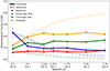 |
Fig. 7. Same as Fig. 6, but for the CANDELS star-forming subsample. |
| In the text | |
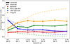 |
Fig. 8. Same as Fig. 6, but for the CANDELS quiescent subsample. |
| In the text | |
|
Fig. 9. Morphological fractions in the TNG50 sample as a function of redshift. The observed morphological fractions are represented as dashed opaque lines, while the CSBD-corrected fractions are represented as solid lines. Likewise CANDELS, the effect of CSBD on the observed morphological fractions of early- and late-type disks and irregulars is significant. |
| In the text | |
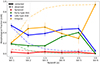 |
Fig. 10. Same as Fig. 9, but for the TNG50 star-forming subsample. |
| In the text | |
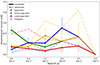 |
Fig. 11. Same as Fig. 9, but for the TNG50 quiescent subsample. |
| In the text | |
|
Fig. 12. Spearman correlation test conducted to quantify the degree of correlation between the variables ΔG and ΔM. The results indicate a significant correlation between the two variables at all redshifts. |
| In the text | |
|
Fig. 13. G − M20 plane as a function of redshift in CANDELS. The estimates of the coefficients obtained from the observed data are plotted in red, while the corrected coefficients are represented in blue, and the coefficients from bin 0 are shown in gray. As a reference, the orange lines displayed on the plot indicate the boundaries defined in Lotz et al. (2008) to classify galaxies into early-type, late-type and mergers in the G − M20 plane. |
| In the text | |
|
Fig. 14. Distributions of G (left column), M20 (middle column), and As (right column) are plotted for bin 1 (top row), bin 3 (middle row), and bin 6 (bottom row), respectively. The red histograms represent the observed values and the blue represent the CSBD-corrected values. The distribution of coefficients measured in bin 0 is plotted as a green histogram. It can be seen that in bin 1 the corrected and uncorrected distributions appear similar, suggesting that the impact of CSBD is negligible. However, in bin 6, a more pronounced difference between the observed and corrected values is evident. |
| In the text | |
|
Fig. 15. Morphological fractions as a function of redshift in CANDELS obtained with the G − M20 − As classification. Solid lines refer to CSBD corrected values, while dashed lines refer to the observed values. It can be seen that the difference between observed and corrected fractions is small. |
| In the text | |
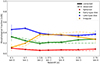 |
Fig. 16. Same as Fig. 15, but for star-forming galaxies. |
| In the text | |
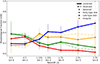 |
Fig. 17. Same as Fig. 15, but for quiescent galaxies. |
| In the text | |
|
Fig. 18. Morphological fractions obtained with method 2 plotted as a function of stellar mass in CANDELS. Each panel represents a morphological type, and the values in each redshift bin are plotted in the same color. The dashed lines correspond to the observed, uncorrected fractions. |
| In the text | |
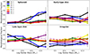 |
Fig. 19. Same as Fig. 18, but for the star-forming subsample. |
| In the text | |
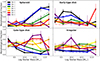 |
Fig. 20. Same as Fig. 18, but for the quiescent subsample. |
| In the text | |
|
Fig. 21. Median and 1σ widths of the distributions of the observed (red) G, M20, As, and half-light radius (Re) are displayed from top to bottom in each panel. The median of the corrected G, M20 and As values are shown as blue lines. |
| In the text | |
|
Fig. 22. Morphological fractions as a function of redshift in TNG50 estimated with method 2. The observed and corrected fractions are shown in dashed lines and solid lines, respectively. |
| In the text | |
|
Fig. 23. Morphological fractions estimated with method 2 as a function of stellar mass in TNG50. Each panel represents a morphological type, and the values in each redshift bin are plotted in the same color. The dashed lines correspond to the observed, uncorrected fractions. |
| In the text | |
|
Fig. 24. Over- and underestimation of the observed morphological fractions in CANDELS as a function of redshift. Dotted, dashed and solid lines represent the low-stellar mass sample (M* < 1010 M⊙), high-stellar mass sample (M* ≥ 1010 M⊙) and the entire sample, respectively. The y-axis represents the difference between the observed and corrected fractions. So all the values within the light-gray region correspond to underestimations of the morphological fractions, while the white area indicates the overestimation. Notably, the differences between the observed and corrected fractions increase with redshift, with the exception of the spheroid class. |
| In the text | |
|
Fig. 25. Three example images of artificially redshifted galaxies. Top row: images of three galaxies from the reference sample at bin 0, a spheroid, an early-type disk, and an irregular. Bottom row: redshifted versions of the galaxies in bin 6 (z ∼ 2.75). Each panel shows the morphological coefficients estimated for a galaxy in the bottom left corner and its segmentation image in the top right corner. Despite the evident change in visual appearance, the variations in the morphological coefficients are small. |
| In the text | |
|
Fig. 26. Morphological fractions as a function of redshift from published works. The plot includes Conselice et al. (2005; blue), Lotz et al. (2004; red), Mortlock et al. (2013; green), Whitney et al. (2021; purple), Margalef-Bentabol et al. (2022; yellow), Ferreira et al. (2022; orange), Huertas-Company et al. (2023; pink), and Jacobs et al. (2023; turquoise). The observed morphological fractions in this study are plotted in dark red, and the corrected morphological fractions obtained with Method 1 and Method 2 are plotted in gray and black, respectively. |
| In the text | |
Current usage metrics show cumulative count of Article Views (full-text article views including HTML views, PDF and ePub downloads, according to the available data) and Abstracts Views on Vision4Press platform.
Data correspond to usage on the plateform after 2015. The current usage metrics is available 48-96 hours after online publication and is updated daily on week days.
Initial download of the metrics may take a while.