| Issue |
A&A
Volume 682, February 2024
|
|
|---|---|---|
| Article Number | A12 | |
| Number of page(s) | 6 | |
| Section | Catalogs and data | |
| DOI | https://doi.org/10.1051/0004-6361/202348125 | |
| Published online | 29 January 2024 | |
Methodology for obtaining the relative orbit and individual masses of Gaia astrometric binaries★
1
Centro de Investigación e Tecnoloxía Matemática de Galicia (CITMAga),
15782
Santiago de Compostela,
Galiza,
Spain
2
Observatorio Astronómico R. M. Aller (OARMA), Universidade de Santiago de Compostela (USC),
Campus Vida,
15782
Santiago de Compostela,
Galiza,
Spain
e-mail: xabier.perez.couto@usc.es; joseangel.docobo@usc.es
3
Agrupación Astronómica Coruñesa 'Ío',
15005
A Coruña,
Galiza,
Spain
4
Real Academia de Ciencias de Zaragoza, Facultad de Ciencias,
C/ Pedro Cerbuna 12,
50009
Zaragoza,
Spain
5
Observatorio Astronómico Nacional,
C. de Alfonso XII, 3,
28014
Madrid,
Spain
e-mail: p.campo@oan.es
Received:
2
October
2023
Accepted:
21
November
2023
Context. The recent Gaia Data Release 3 has revealed a catalogue of more than eight hundred thousand binary systems. The release provides orbital solutions for half of the systems, with the majority of them being unresolved astrometric binaries. However, some astrophysical parameters are still unknown for most of them, such as the spectral type and the mass of each companion, since they can only be derived from the relative orbit and spectroscopic data.
Aims. The purpose of this work is to develop a methodology that would allow us to obtain those fundamental stellar parameters, along with those related to the geometry and the ephemeris of the system, to find out whether it can be optically resolved.
Methods. To obtain precise values for each component, we proposed an analytic algorithm to estimate the only two possible relative orbits and pairs of masses of main sequence (MS) astrometric binaries using all the available astrometric, photometric, and spectro-scopic data from Gaia DR3. In some cases, it is possible to select the solution that is more aligned with the rest of the data.
Results. We deduced two possible values for the individual absolute magnitudes, masses, and effective temperatures for each binary, as well as the size of the telescope necessary to resolve their components. We present the workflow of our algorithm applied to the Ephemeris, Stellar Masses, and relative ORbits from GAia (ESMORGA) catalogue, along with the individual masses, absolute magnitudes, and effective temperatures derived for 49 530 binaries.
Key words: methods: data analysis / methods: numerical / astrometry / binaries: general
Catalog is available at the CDS via anonymous ftp to cdsarc.cds.unistra.fr (130.79.128.5) or via https://cdsarc.cds.unistra.fr/viz-bin/cat/J/A+A/682/A12
© The Authors 2024
 Open Access article, published by EDP Sciences, under the terms of the Creative Commons Attribution License (https://creativecommons.org/licenses/by/4.0), which permits unrestricted use, distribution, and reproduction in any medium, provided the original work is properly cited.
This article is published in open access under the Subscribe to Open model. Subscribe to A&A to support open access publication.
1 Introduction
Since the orbital motion of binary stars was discovered more than 200 yr ago (Herschel 1803), the study of stellar systems has become a key topic in astronomy. The scope of binary research extends to several areas, including stellar dynamics, stellar evolution, exoplanetology, and galaxy mapping, since the determination of the individual masses of the system from calculated binary orbits allows for its evolution to be studied. In addition, binary orbits provide a good distance estimation tool, namely, the dynamical parallax (Heintz 1978).
The observational techniques that allow the greatest numbers of orbits to be calculated are speckle interferometry (Labeyrie 1970; Balega & Tikhonov 1977; McAlister 1983), adaptive optics (Babcock 1953), and space surveys (Perryman et al. 1997; Gaia Collaboration 2023). In this work, we focus on the latest data release of the Gaia mission: Gaia DR3.
The high accuracy of the positions and proper motions afforded by Gaia has allowed for detections of an unprecedented 338 215 astrometric binary stars, with orbital solutions for 145 259 of them to date. However, since the astrometric orbit shows the movement of the photocentre of the system around its centre of mass (rather than the orbital motion of one component around the other), the Gaia table of binary masses (gaiadr3.binary_masses) only includes estimates  and
and  of the individual masses of main sequence (MS) components if a spectroscopic orbit is also available (as it occurs for 33 467 AstroSpectroSB1 solutions; hereafter noted as: astro-spectroscopic solutions). For the 111792 binaries with only pure astrometric orbits, the
  is given, but for the secondary only an estimated interval,
 ![$\left[ {\widehat {\cal M}_{\rm{B}}^{\min },\widehat {\cal M}_{\rm{B}}^{\max }} \right]$](/articles/aa/full_html/2024/02/aa48125-23/aa48125-23-eq4.png) , has been provided (Gaia Collaboration 2023). Shahaf et al. (2019) proposed an alternative procedure that allows for the primary mass − and thereby two possible mass ratios − to be obtained; however, as the authors indicated, this method ignores the contribution of the secondary component to the photometry of the system.
, has been provided (Gaia Collaboration 2023). Shahaf et al. (2019) proposed an alternative procedure that allows for the primary mass − and thereby two possible mass ratios − to be obtained; however, as the authors indicated, this method ignores the contribution of the secondary component to the photometry of the system.
In this paper, we describe an algorithm that takes into account the photometric contribution of the secondary component of a system, which allows it to yield up to two possible solutions for the individual masses (demonstrating that, in fact, no more than two are possible) when sufficiently good data are supplied. Then, we used additional data from Gaia to achieve the most consonant solution for the individual masses. Finally, the ephemeris of the apparent orbit were obtained, so we could also assess the possibility of resolving the binary. The manuscript is organised as follows. In Sect. 2, we present our methodology, from the theoretical framework to the step-by-step description of the algorithm. The key results obtained by applying the method to Gaia data are shown and discussed in Sect. 3. Finally, our main conclusions are given in Sect. 4.
2 Methodology
2.1 Theoretical framework
As noted above, the orbital solutions given by the Gaia DR3 Non-Single Star (NSS) astrometric solution table correspond to the movement of the photocentre around the centre of mass. That orbit is related to the relative orbit via
 (1)
(1)
where a is the semi-major axis of the photocentric orbit, a″is that of the relative orbit, and f is the mass ratio:
 (2)
(2)
while β is the corresponding flux ratio, defined by
 (3)
(3)
where fG,A and fG,B are the spectral flux densities in the Gaia G-band of both components, and ΔmG is their magnitude difference. Therefore, starting with the α given by the Gaia NSS table, we can calculate a″ if we know the individual masses, ℳA and ℳB, of both companions, as well as their ΔmG. Unfortunately, those three mentioned variables are a priori unknown (in truth, they are among the unknowns that we want to solve). We can use the calibration of Pecaut & Mamajek (2013) for MS stars to obtain the stellar mass from its absolute magnitude or colour. However, it is very often the case that the absolute magnitude of each component is not determined, only the combination of light of both components, known as the combined absolute magnitude, MG.
Inspired by Edwards (1976) and Campo (2019), we performed a decomposition of the overall photometry of the system by expressing MG as an interpolation of the individual magnitudes, MG,A and MG,B, weighted by ΔmG:
 (4)
(4)
with MG,B = MG,A + ΔmG. We still need to know ΔmG to work but now we have it as an input parameter in both Eqs. (1) and (4), so that we can take advantage of that to develop an analytical and recursive algorithm (see Sect. 2.2) to get the set of possible solutions for ΔmG and, thus, the rest of the output parameters.
2.2 Algorithm: Step by step
The algorithm described here is used to obtain a set of candidates for the relative semi-major axis, a″ from the semi-major axis of an astrometric orbit, a. During the process, each solution yields a value for the ΔmG of the unresolved system along with a precise estimate of the individual mass of each component.
Furthermore, we can compute the orbital ephemeris so we can derive straightforwardly the minimum  and maximum
  angular separation between their components. Subsequently, and together with ΔmG, the minimum size that a telescope needs to resolve that system comes to light.
2.2.1 Sample selection and preprocessing
Given an NSS astrometric or astrospectroscopic solution from Gaia DR3, we first have to determine whether its composite spectrum corresponds to an MS star, since the calibrations we will use are only valid for stars with spectral types between B1.5V and L2V. The luminosity class of the input star can be determined using the logarithm of its surface gravity, log g, given in the Gaia DR3 source catalogue as logg_gspphot (in dex). For instance, on the basis of the work of Angelov (1996), Zboril et al. (1997) and Bastien et al. (2016), we could restrict the input MS stars to those with log g ≥ 4.0 dex. However, the surface gravity of an unresolved binary considered as a single star is not very reliable, as the cooler companion gives rise to underestimation of the effective temperature, and, thus, also of log ɡ, which is highly correlated with Teff and metallicity (El-badry et al. 2018; Ting et al. 2017). Therefore, instead of using the surface gravity computed by GSP-Phot on the basis of a single-star model, we redefine log g as the lesser of the Multiple Star Classifier (MSC) individual surface gravities, logg1_msc and logg2_msc, assuming that both components are at the same evolutionary stage and that their flux ratio is smaller than 5. This is the value of log g used to exclude stars that are not on the MS.
Next, the seven Campbell orbital elements for the astromet-ric orbit were derived together with their uncertainties, as fully detailed in Halbwachs et al. (2023). Thereafter, we applied the same filter used in Gaia Collaboration (2023) for discarding low signal-to-noise ratio (S/N) solutions, by imposing S /N > 5 for a and S /N > 2 for sin I in astrometric orbits, while log10(S /N) > 3.7−1.1 log10 P is also required for orbitalAlternative solutions. Moreover, S /N > 5 for  and a1 in the astrospec-troscopic ones is demanded. Next, we go on to describe how the algorithm works, step by step, below.
2.2.2 First step: Photometric decomposition
For each binary, we get its combined absolute magnitude (MG) from the G-band mean apparent magnitude, mG, given by Gaia DR3 as phot_g_mean_mag (mag): after mG is first corrected for interstellar absorption and scattering by subtracting the extinction in the G-band (available as ag_msc (mag)), MG is obtained from the distance-modulus relation using parallax (mas). The initial values for MG,A and MG,B are then obtained by choosing a small enough magnitude difference, e.g. ΔmG = 0.05 mag, and using Eq. (4).
2.2.3 Second step: Initial solution
Subsequently, the method uses the calibration of Pecaut & Mamajek (2013) to compute the individual masses, ℳA and ℳB, by means of a cubic spline interpolation. At the same time, we can use the later ΔmG to calculate the flux ratio, β, by means of the second equality in Eq. (3). Moreover, the mass ratio f is computed from Eq. (2) together with the individual masses, ℳA and ℳB, estimated in the first step. Therefore, we can obtain an initial value for a” that, like a, is measured in arc seconds. This is not a problem because we have the Gaia parallax,  , so that the value of a in au is recovered.
2.2.4 Third step: Again and again
From the value of a derived in the previous step in addition to the orbital period, P, available in the Gaia DR3 NSS astrometric solution, by means of Kepler’s third law, we can determine, the sum of the masses (in this case, referred to as ‘Keplerian masses’, to differentiate them from those obtained with the calibrations),  . On the other hand, by adding up the initial masses, we get ℳT = ℳA + ℳB; it is clear that if the assumed value for ΔmG is correct, then
For that reason, the core idea of the algorithm is to perform the previous set of calculations with different values of ΔmG, until the above equality is verified. Therefore, the algorithm repeat the previous steps increasing ΔmG by 0.05 mag and, by doing this recursively and performing the following multiplication for each i iteration,
 (5)
(5)
it is clear that if it changes its sign then the solution is located in the interval ![$\left[ {\Delta {m_{{\rm{G}},i - 1}},\Delta {m_{{\rm{G}},i}}} \right]$](/articles/aa/full_html/2024/02/aa48125-23/aa48125-23-eq16.png) (see Sect. 3.1 for further details).
(see Sect. 3.1 for further details).
Thus, the process continues until an arbitrarily high ΔmG, e.g. ΔmG = 10 mag, since there can be more than a possible solution. Subsequently, we consider the medium point of each solution interval as an estimator of the ΔmG solution.
2.2.5 Fourth step: Ephemeris calculation
Using the obtained solutions for ΔmG and the mean value of the individual masses (corresponding to the extremes of the interval in which we found the solution) we get, through Kepler’s third law, the relative semi-major axis, a.
From this − and together with the rest of the orbital parameters derived from the Innes constants − we are able to compute the apparent orbit through the widely known ephemeris algorithm (see e.g. Abushattal et al. 2020). Ultimately, the minimum (ρmin) and maximum (ρmax) angular separations between the components are derived, as well as their corresponding dates.
2.3 Evaluating consonance with Gaia DR3
For binaries with pure astrometric orbits in Gaia DR3 we quantify consonance with our possible solutions by assigning to each of the latter a grade defined in terms of the relative difference between  , as follows:
grade = 
grade = 
grade = 
grade = 
grade =  , and so on.
These grades are listed in the catalogue ESMORGA (see Sect. 3.3). The more consonant of our two possible solutions is identified as that with ℳA closer to  , so long as
 ![${\cal M}_{\rm{B}}^j \in \ \ \left[ {\widehat {\cal M}_{\rm{B}}^{\min },\widehat {\cal M}_{\rm{B}}^{\max }} \right].$](/articles/aa/full_html/2024/02/aa48125-23/aa48125-23-eq24.png) .
.
For binaries with astrospectroscopic orbits in Gaia DR3, we assign grades in the same way as above, but using, intead of  , the greater of
  and
and  , which is analogously defined. For these binaries, consonance with Gaia DR3 can also be examined in terms of the binary mass function (fm, in ℳ⊙), which (like the total mass) can be calculated by two routes: firstly, from the Innes constants C1 and H1 provided by Gaia DR3 for astrospectroscopic solutions (Gaia Collaboration 2023):
 (6)
(6)
where C1 and H1 are in au and P in years; and secondly, from the individual masses as
 (7)
(7)
We consider that our solution passes this test of consonance if
 (8)
(8)
This binary mass function test can also be applied to binaries with only pure astrometric orbits in Gaia DR3, using for fm the estimate used by Tanikawa et al. (2023):
 (9)
(9)
where K1 is the RV semi-amplitude of the primary component, approximated as half rv_amplitude_robust. However, this parameter corresponds to RV variability and not to a fitted RV curve, so caution is needed, especially for eccentric orbits.
2.4 Error propagation
Finally, to estimate the propagation of uncertainties σ, we have used the standard Taylor-expansion method to obtain  , assuming
  mag and
  = 0.025 mag. Subsequently, to estimate the error in the non-linear interpolations, we performed 10000 Monte Carlo simulations assuming normally distributed MG errors
  . Taking the mean and standard deviation of the interpolated samples of masses and effective temperatures as the estimates and their uncertainties, respectively, we followed the subsequent propagation of the uncertainty through to the ephemeris by means of partial derivatives.
3 Results and discussion
3.1 Examining the numerical convergence
The process is equivalent to find the zeros of the function:
 (10)
(10)
To study how Δℳ (ΔmG) behaves as we scan through a range of ΔmG values, we ran the algorithm on 796 Gaia DR3 astrometric binaries with well-established combined magnitudes available at SIMBAD1, computing Δℳ for ΔmG ∈ [0.5,8] mag with increments of 0.05 mag.
As can be seen in Fig. 1. the function Δℳ shows an asymmetric parabolic shape that, depending on the star, cut the abscissa axis in different points. The black and green quasi-parabolas show two and one zeros (but maybe one more could be found if we increase the superior limit of ΔmG). There is a straightforward mathematical explanation for this: β decreases by a factor of  , whereas f comes from the quotient of two polynomials of degree 3 (the cubic spline interpolations), so that β will decrease faster at the beginning and therefore a/a″ has a maximum. In Fig. 2, we show this behaviour for a generic Gaia DR3 MS binary. Then, for the same scale factor there are generally two feasible values for ΔmG.
Regarding the no-solution case, corresponding to the blue quasi-parabola that does not touch the abscissa axis, it should be recalled that even though we are evaluating Δℳ as a function of ΔmG, its values also depend on the dynamical (a,  , P) properties of the astrometric binary. Therefore, at one extreme of the spectrum of possibilities, this might be entirely due to the Gaia DR3 photocentre orbit being erroneous; at the other, this could be due to an inappropriate use of the Pecaut-Mamajek calibration, namely, erroneous assumptions as regards the luminosity class of the components.
 |
Fig. 1 Graphical representation of Δℳ for three Gaia DR3 unresolved astrometric binaries, with two solutions (black), a single solution (green), and zero solutions (blue) for ΔmG. |
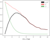 |
Fig. 2 Plot of f, f, β, and a/a″ versus ΔmG for Gaia DR3 5706079252076583424. |
3.2 Validation of the algorithm
To test the algorithm we have cross-matched the Gala’s sources with an astrometric solution with those contained in the Sixth Catalog of Orbits of Visual Binary Stars (WDS-ORB6), using a search radius of 5″. By doing so, we have constrained a set of 26 Gaia astrometric orbits with a resolved orbit in the WDS-ORB6. Then, we have selected those belonging to the MS, attending to SIMBAD and/or to the log(ɡ), and filtering them by means of the 10σ-criteria used in Chevalier et al. (2023) to discard different orbits within the same multiple system.
The comparison on the resulting 10 semi-major axes is shown in Table 1. By using the similarity criteria with  and
and  , or the fm to constrain the most consonant solution (see bold rows in Table 1), the relative discrepancy is 7−10%, respectively. The problem arises when comparing the ΔmG obtained by our algorithm with that of the ORB6. For each pair of solutions, there is one that is close to the ORB6 Δmv, whereas for WDS 09275-5806, 18040+0150, and 12114-1647, neither the Gaia masses nor fm selecting criteria seem to work. This holds true whether we calculate the fm with rv_amplitude_robust or with C1 and H1 (for AstroSpectroSB1 solutions), in which case the binary mass function calculation is especially strong. Therefore, if we accept the ground-based measurements as benchmarks, the Gaia data used to compute those SB1 orbits and masses may benefit from some revision.
3.3 Application on the Gaia DR3 astrometric orbits: ESMORGA catalogue
By means of the criteria described in Sect. 2.2.1, we selected an initial sample of 82 759 astrometric binaries. By applying the algorithm to all of them, with ΔmG ∈ [0.05, 20] mag in steps of 0.05 mag, we obtained solutions for a total of 52 678 systems. Subsequently, this set was reduced to 49 530 by choosing only those with individual masses and binary mass functions in consonance with the Gaia values. Finally, we have included these latter in the catalogue ESMORGA (Ephemeris, Stellar Masses and relative ORbits from GAia), which can be downloaded from the Ramon María Aller Astronomical Observatory website2. The full table will be made available on VizieR. Here, we present a description of the catalogue, column by column.
3.3.1 Description of the catalogue
Each binary corresponds to a row, while the uncertainties are shown in the row below. If two possible solutions for the binary are provided, they appear in consecutive rows. The columns with the parameters per source are organised as indicated in Table 2.
3.3.2 Catalogue statistics
The catalogue provides just a single solution for 10 643 binaries, 21.5% of the total, and 39 639 binaries are marked as grade 1. Several binary parameters can be thus studied, being the separations between the astrometric companions the most straightforward one. In Fig. 3, the density histogram of the semi-major axes in au is shown in red. The sample reaches the 99th percentile to enhance data visualization. As can be seen, Gaia astrometric binaries are very close, with separations within the Solar System scale, most of them having a semi-major axis between 0.5 and 2 au. Moreover, there is a deep decay around 1 au that, by comparison with the histogram of the periods (blue), shows to be associated with the Gaia s observational bias for binary orbits of 1 yr, which is due to the coupling of the orbital and parallactic motions (Gaia Collaboration 2023).
In the case of astrospectroscopic orbits, a1 is straightforwardly obtained and, by means of the following relation,
 (11)
(11)
the semi-major axis of the secondary component around the centre of mass, a2 = a1 ℳA/ℳB, is known. Then, we can derive an alternative semi-major axis  and, from it, another for the parallax
  (hereafter, the astrospectroscopic parallax).
It is clear that, if the relative orbit aligns with the Gaia spectroscopic one, then  . Indeed, from the comparison of the 3714 single-solution astrospectroscopic parallaxes of grade ‘1*’ and ‘2*’ with those of Gaia, there is a mean absolute discrepance of 0.8 mas (std = 2.6 mas) for grade ‘1*’, and 1.9 mas (std = 3.2 mas) for grade ‘2*’. This may be considered as an additional validation for astrospectroscopic solutions.
Finally, we present a histogram in Fig. 4 displaying the masses of primary and secondary components up to the 99.9th percentile, although the maximum mass obtained was 2.76Aℳ⊙ for a primary and 1.78 ℳ⊙ for a secondary, while the minimum masses correspond to a primary of 0.09ℳ⊙ and a secondary of 0.08 ℳ⊙.
Comparison between the semi-major axis of ten visual binaries found in the WDS-ORB6 and those computed by our algorithm
ESMORGA catalogue content, column by column.
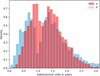 |
Fig. 3 Density histogram of a and P for 10 643 binaries. |
 |
Fig. 4 Mass distribution of the primaries (blue) and secondaries (red). |
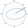 |
Fig. 5 Apparent orbit of Gaia DR3 1724494760222303872. The radial coordinate, ρ, is in arc seconds and θ = 0° in the north. |
3.4 Example of use in resolving an unresolved astrometric binary
As commented in Sect. 2.2.5, the algorithm allows to draw the apparent orbit of the secondary companion around the primary for any unresolved astrometric binary, as can be seen in Fig. 5. In this case, ΔmG = 0.78 mag, ρmin = 30.4 + 0.3 mas in 2024.36, and ρmax = 69.1 + 0.4 mas in 2024.88. Accordingly, a telescope of between 4 and 1.8 m would be required, respectively, to resolve it, depending on the observation date (see e.g. Tokovinin et al. 2022).
4 Conclusions
We have developed and implemented a novel algorithm to calculate the only two possible semi-major axes for the relative orbit of MS unresolved astrometric binaries. A unique solution can be obtained if additional spectroscopic data such as an SB 1 orbit or a reliable RV amplitude is available. Through our procedure, based on the decomposition of the combined photometry, we are able to determine precise values for decisive astrophysical parameters such as the masses and effective temperatures of each component. Moreover, the ephemerides of the calculated apparent orbits of these systems provide the maximum and minimum angular separations between the components, which, in turn, can be used to evaluate the feasibility of resolving them. The results for 49 530 binary systems using this methodology are presented in the ESMORGA catalogue.
We have validated our algorithm by comparing its results for the semi-major axis with ten orbits in the catalogue WDS-ORB6. The algorithmic semi-major axes differ, on average, by less than 10% from the ground-based ones, while for ΔmG we have found contradictory clues on that computed by the algorithm and the mass ratio of the Gaia binary mass table; thus, more observations over more astrometric systems must be carried out to improve on these results. On the other hand, the stellar masses computed by our methodology are in high consonance (mostly, grade = 1) with those calculated in Gaia Collaboration (2023), which validates the procedure and allows us to choose (when needed) the most plausible solution between those two provided in the first instance by the methodology. However, we recommend taking into account additional data whenever possible to choose the definitive solution.
We aim for this work to serve as a supplementary tool to exploit the enormous amount of astrometric and astrophysical data provided by Gaia and future astrometric missions. We expect that its application to the forthcoming Gaia Data Release 4 should allow us to choose the preferred solutions with more confidence, thanks to the growing number of released observations and more robust RV amplitudes.
Acknowledgements
The authors thank the referee, Andrei Tokovinin, for his valuable comments and suggestions that have served to improve the performance of the algorithm. This work presents results from the European Space Agency (ESA) space mission Gaia. Gaia data are being processed by the Gaia Data Processing and Analysis Consortium (DPAC). Funding for the DPAC is provided by national institutions, in particular the institutions participating in the Gaia Multi-Lateral Agreement (MLA). The Gaia mission website is https://www.cosmos.esa.int/gaia. The Gaia Archive website is http:/archives.esac.esa.int/gaia. Another catalogues and databases that have been crucially important for the preparation of this work, are: the Washington Double Star Catalog (WDS) and the Sixth Catalog of Orbits of Visual Binary Stars (ORB6), maintained by the US Naval Observatory (USA, https://crf.usno.navy.mil/wds); the SIMBAD database, operated by the Centre de Don-nees astronomiques de Strasbourg (France, http://simbad.cds.unistra.fr/simbad/); and the Astrophysics Data System (NASA/SAO, https://ui.adsabs.harvard.edu/). This paper was supported by the Spanish ‘Min-isterio de Ciencia e Innovation’ under the Project PID2021-122608NB-I00 (AEI/FEDER, UE), and by the European Union under the INVESTIGO (Next Generation) grant.
References
- Abushattal, A. A., Docobo, J. A., & Campo, P. P. 2020, AJ, 159, 28 [Google Scholar]
- Angelov, T. 1996, Publ. Astron. Obs. Belgrade, 154, 13 [Google Scholar]
- Babcock, H. W. 1953, PASP, 65, 229 [NASA ADS] [CrossRef] [Google Scholar]
- Balega, Y. Y., & Tikhonov, N. A. 1977, Sov. Astron. Lett., 3, 272 [Google Scholar]
- Bastien, F. A., Stassun, K. G., Basri, G., et al. 2016, Apl, 818, 43 [Google Scholar]
- Campo, P. P. 2019, PhD Thesis. USC, Galiza, Spain [Google Scholar]
- Chevalier, S., Babusiaux, C, Merle, T., & Arenou, F. 2023, A&A, 678, A19 [NASA ADS] [CrossRef] [EDP Sciences] [Google Scholar]
- Edwards, T. W. 1976, Al, 81, 245 [NASA ADS] [Google Scholar]
- El-Badry, K., Rix, H.-W., Ting, Y.-S., et al. 2017, MNRAS, 473, 5043 [Google Scholar]
- Gaia Collaboration (Arenou, F, et al.) 2023, A&A, 674, A34 [CrossRef] [EDP Sciences] [Google Scholar]
- Gaia Collaboration 2023, Gaia Data Release 3 documentation, ESA [Google Scholar]
- Halbwachs, l.-L., Pourbaix, D., Arenou, F., et al. 2023, A&A, 674, A9 [NASA ADS] [CrossRef] [EDP Sciences] [Google Scholar]
- Heintz, W. D. 1978, Double Stars, Geophys. Astrophys. Monogr. (Dordrecht: Reidel) [CrossRef] [Google Scholar]
- Herschel, W. 1803, Philos. Trans. R. Soc. Lond., 93, 339 [NASA ADS] [Google Scholar]
- Labeyrie, A. 1970, A&A, 6, 85 [Google Scholar]
- McAlister, H. A. 1983, IAU Colloquium 62, 125 [NASA ADS] [Google Scholar]
- Pecaut, M. I., & Mamajek, E. E. 2013, ApJS, 208, 9 [NASA ADS] [CrossRef] [Google Scholar]
- Perryman, M. A. C, Lindegren, L., Kovalevsky, I., et al. 1997, A&A, 323, 49 [NASA ADS] [Google Scholar]
- Shahaf, S., Mazeh, T., Faigler, S., et al. 2019, MNRAS, 487, 5610 [NASA ADS] [CrossRef] [Google Scholar]
- Tanikawa, A., Hattori, K., Kawanaka, N, et al. 2023, Apl, 946, 79 [Google Scholar]
- Ting, Y., Conroy, C., Rix, H., & Cargile, P. 2017, Apl, 843, 32 [Google Scholar]
- Tokovinin, A., Mason, B. D., Mendez, R. A., & Costa, E. 2022, Al, 164, 58 [NASA ADS] [Google Scholar]
- Zboril, M., North, P., Glagolevskij, Y. V., et al. 1997, A&A, 324, 949 [NASA ADS] [Google Scholar]
All Tables
Comparison between the semi-major axis of ten visual binaries found in the WDS-ORB6 and those computed by our algorithm
All Figures
|
Fig. 1 Graphical representation of Δℳ for three Gaia DR3 unresolved astrometric binaries, with two solutions (black), a single solution (green), and zero solutions (blue) for ΔmG. |
| In the text | |
|
Fig. 2 Plot of f, f, β, and a/a″ versus ΔmG for Gaia DR3 5706079252076583424. |
| In the text | |
|
Fig. 3 Density histogram of a and P for 10 643 binaries. |
| In the text | |
|
Fig. 4 Mass distribution of the primaries (blue) and secondaries (red). |
| In the text | |
|
Fig. 5 Apparent orbit of Gaia DR3 1724494760222303872. The radial coordinate, ρ, is in arc seconds and θ = 0° in the north. |
| In the text | |
Current usage metrics show cumulative count of Article Views (full-text article views including HTML views, PDF and ePub downloads, according to the available data) and Abstracts Views on Vision4Press platform.
Data correspond to usage on the plateform after 2015. The current usage metrics is available 48-96 hours after online publication and is updated daily on week days.
Initial download of the metrics may take a while.