| Issue |
A&A
Volume 682, February 2024
|
|
|---|---|---|
| Article Number | A84 | |
| Number of page(s) | 10 | |
| Section | Astronomical instrumentation | |
| DOI | https://doi.org/10.1051/0004-6361/202346929 | |
| Published online | 07 February 2024 | |
A strategy for sensing the petal mode in the presence of AO residual turbulence with the pyramid wavefront sensor
1
DOTA, ONERA, Université Paris Saclay,
91123
Palaiseau,
France
e-mail: This email address is being protected from spambots. You need JavaScript enabled to view it.
2
INAF – Osservatorio Astronomico di Arcetri,
50125
Firenze,
FI,
Italy
3
Aix-Marseille Univ, CNRS, CNES, LAM,
13013
Marseille,
France
4
University of California Santa Cruz,
1156 High St,
Santa Cruz,
USA
5
IFREMER, Laboratoire Détection, Capteurs et Mesures (LDCM),
Centre Bretagne, ZI de la Pointe du Diable, CS 10070,
29280
Plouzane,
France
Received:
17
May
2023
Accepted:
22
October
2023
Abstract
Context. With the Extremely Large Telescope (ELT) generation of telescopes come new challenges. The complexity of these telescopes’ pupils creates new problems for adaptive optics (AO) that prevent the telescopes from reaching the theoretical resolutions that their size allows. In particular, the large spiders necessary to support the massive optics of these telescopes create discontinuities in the wavefront measurement. These discontinuities appear as a new phase error dubbed the “petal mode.” This error is described as a differential piston between the fragment of the pupil separated by the spiders and is responsible for a strong degradation in the imaging quality, reducing the European ELT’s resolution to that of a 15m telescope.
Aims. The aim of this paper is to study the measurement of the petal mode by AO sensors. In particular, we want to understand why the pyramid wavefront sensor (PyWFS), the first-light wavefront sensor of any ELT-generation telescope, cannot measure this petal mode under normal conditions, and how to enable this measurement by adapting the AO control scheme and the PyWFS.
Methods. To facilitate our study, we considered a simplified version of the petal mode, featuring a simpler pupil than the ELT. This allowed us to quickly simulate the properties of the petal mode and its measurement by the PyWFS. We studied specifically how a system that separates the atmospheric turbulence from the petal measurement would behave. Studying the petal mode’s power spectral density, we proposed using a spatial filter to reduce the contribution of AO residuals to the benefit of petal mode contribution, eventually enabling it to be measured. Finally, we demonstrated our proposed system with end-to-end simulations.
Results. A solution proposed to measure the petal mode is to use an unmodulated PyWFS (uPyWFS), but the uPyWFS does not make accurate measurements in the presence of atmospheric residuals. A spatial filtering step, consisting of a pinhole around the pyramid tip, reduces the first path residuals seen by the uPyWFS and restores its accuracy. This system was able to measure and control the petal mode during the end-to-end simulation.
Conclusions. To address the petal problem, a two-path AO with a sensor dedicated to the measurement of the petal mode seems necessary. The question remains as to what could be used as the second path petalometer. Through this paper, we demonstrate that an uPyWFS can confuse the petal mode with the residuals from the first path. However, adding a spatial filter on top of said uPyWFS makes it a good petalometer candidate. This spatial filtering step makes the uPyWFS less sensitive to the first path residuals while retaining its ability to measure the petal mode.
Key words: instrumentation: adaptive optics / methods: numerical / telescopes
© The Authors 2024
 Open Access article, published by EDP Sciences, under the terms of the Creative Commons Attribution License (https://creativecommons.org/licenses/by/4.0), which permits unrestricted use, distribution, and reproduction in any medium, provided the original work is properly cited.
This article is published in open access under the Subscribe to Open model. This email address is being protected from spambots. You need JavaScript enabled to view it. to support open access publication.
1 Introduction
Due to atmospheric turbulence, building a telescope bigger than 15 cm in visible light improves only its capacity to collect more light, not its angular resolution. Telescopes bigger than this threshold have to use adaptive optics (AO) to compensate for the effect of the atmosphere before the light reaches the science instruments. This AO compensation step allows one to restore the diffraction limit and the gain in resolution offered by a larger primary pupil. The next generation of 30m-class telescopes is under construction and will have AO capability from the first light. In particular, in this paper, we focus on the Extremely Large Telescope (ELT; Cayrel 2012).
To meet the challenge of the size of these new telescopes, the classical AO wavefront sensor (WFS), the Shack-Hartmann (SH), is less adapted. Its separation of the pupil into multiple subpupils makes it less sensitive for each subpupil, as shown by Vérinaud (2004). To produce a diffraction-limited point spread function (PSF) on a larger telescope, the number of actuators and, consequently, the number of subpupils required for the measurement increase. The SH becomes more susceptible to noise, and hence not adapted to low-flux regimes. Furthermore, the SH needs more pixels to the point where it is not compatible with current AO cameras. As a result, the SH is being replaced by a new kind of WFS for single conjugated adaptive optics (SCAO), where our only source of light is a natural guide star (NGS). This kind of WFS is called a pyramid wavefront sensor (PyWFS), proposed by Ragazzoni (1996), and is employed in the SCAO mode of each 30 m-class telescope.
The utility of SCAO is to provide high-quality wavefront correction near a bright NGS. Specifically, the most demanding science case for such a system is the search for exoplanets, which requires high AO performance to detect faint objects close to their stars. The PyWFS allows the ELT-class telescopes to reach their diffraction limit and angular resolution with fainter targets than a SH.
Simulations of the HARMONI SCAO module taking the ELT pupil and the segmented M4 (Schwartz et al. 2018a) showed a new limit to the SCAO performances, with differential piston appearing between the pupil fragment separated by the large spiders of the ELT. This is due to the inability of the SCAO system to measure this differential piston and the absence of constraints on this differential piston with a segmented deformable mirror (DM). Owing to its occurrence in multiple systems, this effect has been specifically termed the “petal mode basis,” which is a linear combination of the differential pistons between the pupil fragments. This effect can be greatly reduced by adding constraints on the ELT deformable mirror, using techniques such as minioning (originally called slaving) or a continual DM basis (Bertrou-Cantou et al. 2020).
This adjustment reduces the differential piston to an atmospheric turbulence contribution under the spider rather than across the entire pupil. In this configuration, the turbulence is predominantly influenced by the size of the spider, and the r0. In Fig. 1, we simulate how the petal residuals of an AO loop using a modulated pyramid are impacted by the petal mode with min-ioning of the DM actuators (done in the simulation by using a continuous DM). In particular for the ELT-sized spider at 50 cm, with 15 cm r0 (not plotted), we observe mean petal residuals of 80 nm peak-to-valley (PTV) in residual phases (=40 nm rms). When we correct by the amplitude change caused by  , as shown in Fig. 1 we see that the amplitude of petal is directly proportional to the phase amplitude of the atmosphere. For the current SCAO instruments, this level of petal residuals falls within error budgets.
There are multiple questions about the origin of the petal mode and ways to mitigate it. One possibility is to study the efficiency of different reconstructors. As this paper is tackling the petal problem by improving the sensor’s measurement of the petal mode, we used the simplest wavefront reconstruction available for our sensor: a matrix linear reconstruction using an intensity map, as presented in Fauvarque et al. (2016). It has been shown by Bertrou-Cantou (2021) that an MMSE reconstructor exhibits similar performances to a minioned DM basis with a linear reconstructor, as reported in Schwartz et al. (2018b). Notably, using a sensor that is not sensitive to the petal mode – such as the Shack–Hartmann in a centre of gravity measurement mode, or when the subapertures are smaller than the spider – can still significantly reduce the petal mode. However, the petal will achieve errors comparable to the remaining petal flares in a minioning system, as observed in Bonnefond et al. (2016).
We detail in Sect. 2.2 the different sources of petal modes and why this approach is not suited for all of them. While effective for first-light instruments with purely atmospheric turbulence as the wavefront error, this method will not be adequate for all sources of petal mode. Additionally, it will not meet the error budget for second-generation instruments equipped with extreme adaptive optics (EXAO).
This paper aims to understand why the PyWFS cannot measure the petal mode and to propose a second path in the AO system dedicated to petal mode sensing. We separate here the problem of the ELT phasing of the segments of the ELT (the 798 × 1.45 m hexagonal mirrors that we do not consider) and the phasing of the fragments of the pupil (the six areas separated by the spiders). This would allow the measurement of the residual petal mode after minioning and the measurement of the exterior petal mode like the low wind effect (LWE; explained in Sect. 2.3), allowing EXAO instruments into the ELT. For the system to be quickly adaptable to an ELT instrument, we used the same wavelength constraint as the HARMONI instrument, with a sensing wavelength of 850 nm. As it must measure the fast-evolving atmospheric turbulence petal modes, it needs to be an AO-type sensor with a high sensitivity and linear reconstruction, so we start with the already-used AO sensor as the baseline for this paper.
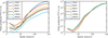 |
Fig. 1 Petal mode with variable r0 and spider size. Left: Petal variation for large spiders and variable r0 in first-stage residuals. For spiders larger than the pitch of the ELT DM, the petal mode increases quickly. Right: Petal variation for large spiders and variable r0 in first-stage residuals corrected of the atmospheric turbulence amplitude. |
2 State of the problem: the petal mode
2.1 Petal properties
To reach the diffraction limit the petal mode would need to be lower than a few tens of nanometers in the residuals.
An uncorrected petal mode creates light residuals in the PSF comparable to slit interference patterns. The resolution on long exposure (with a completely uncorrected petal mode) is then limited not by the size of the pupil of the telescope, but by the size of one fragment (≈15rn). This means the petal mode can be responsible for a loss of resolution up to  . With the atmospheric petal only, the loss of resolution is not of this order, as the mode does not reach high values. However, the LWE petal is expected to reach values over λ. From the differential piston between each fragment, we can define a petal mode basis constituted of five orthogonal petal modes for the ELT (as appears in Bertrou-Cantou et al. 2022). One particularity of the petal mode is that, although it appears in the residual after an AO stage, it can be projected on modes that are measured and compensated by the AO stage. The most obvious is tip-tilt, onto which a lot of the ELT petal modes (or the one from our simplified pupil seen in Fig. 2) can be projected. One might be tempted to orthogonalize this petal mode with the other mode of the basis. As the petal mode can be described in phase space as a Heaviside function, this can be done with an infinity of modes. The resulting petal, orthogonalized to a Zernike mode basis, will tend to a discontinuity phase mode around the spider. The orthogonalized petal mode resulting from this operation has become very different from the mode appearing in AO residuals, such as Schwartz et al. (2018b). To preserve the same mode as our studied mode, we chose to retain the original differential piston petal mode definition. However, to avoid confusion with other modes during phrase reconstruction, we also calibrated the basic Zernike modes (like tip-tilt, see Sect. 3.2 for more details). To simplify the problem, we considered a pupil with only one spider and, consequently, only one petal mode.
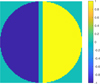 |
Fig. 2 Toy model petal mode. |
2.2 Toy model
For a simplification of the problem, we studied a simplified pupil with a single spider and only two fragments, and therefore only one petal mode. This simple case scaled to a 10 m diameter telescope can be simulated with a coarser sampling and considerably reduces our computational time. To keep the representativity of the ELT case it uses the following parameters: 50 cm spider size and 20 × 20 DM (the same pitch of a DM actuator = 50 cm as the ELT M4).
The petal mode is shown in Fig. 2. We note that this petal is defined with an rms amplitude of 1 radian, and thus has a PTV of 2 radians between the left and right fragments. To stay consistent throughout this article, we use an rms unit for the petal mode. With this normalization, an amplitude of π radians rms means a PTV of 2π radians, hence a λ OPD wrap.
2.3 Sources of the petal mode
As was shown by Bertrou-Cantou (2021), the petal mode is badly sensed by the modulated PyWFS. This means an effect akin to the waffle mode can appear where the mode is amplified by the reconstruction of the AO. Furthermore, if the DM can create this mode, it will create loop instabilities. As the petal mode in this case comes from the AO loop and in particular its control, it evolves as fast as the AO correction. It is currently solved by a technique called minioning (Bond et al. 2022). This technique acts on the control part of the AO loop by forbidding the creation of any differential piston by the DM. The remaining error is the atmospheric petal that exists under the spider. This residual atmospheric petal’s amplitude depends on the size of the spider and the r0 as was shown in the introduction in Fig. 1. There are two problems with this approach. First, this approach only works for atmospheric turbulence petalling. As the petal is not measured if it comes from other sources than atmospheric turbulence, it will not fall within the acceptable first-light instrument constraints. Then for the EXAO system, this is not an acceptable level of residual wavefront error. For a coronographic system, for instance, while it is possible to design coronographs less impacted by this type of wavefront error (Leboulleux et al. 2022), it comes at the cost of the inner working angle.
Another source of petal mode in the phase is the LWE. This is a phenomenon that was discovered on the VLT during the first light of the SPHERE instrument and described in Sauvage et al. (2015). This effect was mitigated on the VLT by improving the emissivity of the spider (i.e., the temperature of the spider is close to the temperature of the environment), but with the larger spiders of the ELT-class telescopes, the LWE is expected to be stronger. A simulation of the airflow around the spiders has recently shown a 1 µm OPD around the spiders, according to Martins et al. (2022), much larger than the petal residual after minioning. As the LWE is poorly understood, we consider it in this paper only as an uncontrolled source of petal mode. It appears in the end-to-end simulation as a brutal petal mode appearing in the phase. It is to be separated from the atmospheric petal as it is a perturbation created by the telescope and not by the atmosphere, though the final phase mode is equivalent.
2.4 Wavefront sensing measurement problem
The petal mode being a differential piston means that in monochromatic light the whole phase screen wraps every λ. This makes a petal larger than λ impossible to detect correctly with a monochromatic sensor, and thus the petal mode has a built-in limit to its range of measurements. This comes back to a phase-unwrapping problem, which we put to one side in the study presented here. In this paper, we only consider monochromatic light and test whether a measurement can be done accurately in ELT conditions.
2.5 Solutions proposed to the petal problem in the literature
Any slope sensor will not be able to measure the petal mode in a subpupil. This is not a problem when the spiders are small, like on the VLT where the petal created by the spiders is negligible. But with 50cm spiders, it becomes a mode large enough to decrease EXAO performances. Phase sensors like the Zernike wavefront sensor (ZWFS) or the unmodulated PyWFS (uPy-WFS) have been proposed as their intrinsic response is more sensitive to phase discontinuities. However, their dynamic is not large enough to measure the atmosphere at the same time.
There are two ways to solve the petal problem proposed in the literature: modify the AO wavefront sensor, or add an additional sensor dedicated to measuring the petal mode, a petalometer. The first solution appears in the METIS instrument. This instrument senses the wavefront at a longer wavelength. Thanks to a lower turbulence phase and a more linear sensor, it doesn’t show any petal mode in its residuals (see Hippler et al. 2019 and Carlomagno et al. 2020). Another solution is the flip-flop method proposed by Engler et al. (2022), where the modulation of the PyWFS is cut to use a temporary uPyWFS and measure the petal mode in the residual.
The GMT has opted for the second solution with the development of the holographic dispersed fringe sensor (HDFS, see Haffert et al. 2022), a sensor dedicated to the phasing of the GMT mirrors.
Moving all AO systems to IR looks like a simple solution but there are a lot of advantages to keeping the sensing in the visible light. IR detectors are slower and noisier than their visible counterparts, meaning fainter stars can be used as NGS by visible systems. Astronomical observations are mainly using IR for most of the first-light instruments. We make our simulation with the wavelength used in the HARMONI instrument: 850 nm. We instead study the petalometer approach in the rest of this paper.
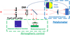 |
Fig. 3 2-Path sensor scheme considered. The green path is dedicated to atmosphere wavefront sensing and features a modulated PyWFS and a classical 20×20 actuator DM. The blue path is dedicated to the sensing of the petal mode, features an uPyWFS, and controls only the petal mode of the DM. |
3 Measurement of petal mode in AO residuals
3.1 2-Path AO system
As was shown by Bertrou-Cantou (2021), the uPyWFS produces a strong signal for the petal mode, even in the presence of a spider, compared to the modulated PyWFS. However, it is not able to measure the petal mode accurately among the whole atmospheric turbulence for a realistic r0. We proposed instead to use the uPyWFS to measure the petal mode among the residuals of an AO loop, as a petalometer. The question in this part is whether the uPyWFS can accurately reconstruct the petal mode among AO residuals. To test this capability, we analyzed the petal mode reconstructed by the PyWFS used as a petallometer, with the 2path system shown in Fig. 3.
There is a single DM correcting the aberrations in the AO loop. This mirror is described by a modal basis, including a pure petal mode of our toy model pupil, as well as the Gaussian influence functions of a 20 × 20 regular actuator grid. The Gaussian influence functions are controlled by the modulated PyWFS and are dedicated to the atmospheric turbulence compensation. The second path includes a petalometer that controls the pure petal mode of the DM. Diverse sensors could be proposed as petalometers for the second path. As we knew that the uPyWFS is a possible alternative in terms of sensing, we used it in this first test. The uPyWFS only controls the petal mode though it can measure other modes.
The first source of the petal mode is atmospheric turbulence. We used this configuration to take advantage of the reduced atmospheric petal mode in the residuals after a first stage using a minioning DM. The petalometer aims to measure and allow the control of both atmospheric petals and the LWE. We also added a fixed petal after some iterations to simulate the LWE.
3.2 uPyWFS petal mode reconstruction
We used the intensity map method described in Fauvarque (2017), so using all the pixels. The linearity curves presented later were reproduced with the slopes map method and give the same results. There does not seem to be a preferred method for measuring the petal mode. The first step was to calibrate the interaction matrix of our system. We created this interaction matrix by simulating the intensity map for a variety of modes. For the atmospheric control, the calibrated phase modes are the zonal base of the 400 actuators. For the petal mode interaction matrix, we needed not only to measure the petal mode but also other Zernike modes, in particular tip and tilt, to avoid confusion between these low-order modes and the petal modes. In practice, we calibrated a modal basis containing the petal mode and 30 Zernike phase modes.
 (1)
(1)
with I(ϕ) the intensity on the PyWFS detector for a given phase, ϕ, and є a factor small enough to work in the linear regime of the PyWFS. In the simulation, we used 10−10. δI(ϕ) is the push-pull intensity map of the mode, ϕ.
 (2)
(2)
see Eq. (1) for the computation of δI(ϕ1). The interaction matrix was then inverted using a Moore–Penrose pseudo inverse to get the control matrix, D†. We used a conditioning number of 100. Assuming a small phase, we should have the relationship
 (3)
(3)
We express any phase as its decomposition on the modal basis used,
 (4)
(4)
with ai being the amplitude of the mode, ϕi.
 (5)
(5)
with âi being the estimated amplitude of the mode, ϕi.
3.3 Linearity curve of petal mode reconstruction
We wanted to test the measurement of the petal mode with a PyWFS used as a petalometer. To that end, we computed the linearity curve to a petal mode, first without AO residuals to set the ideal case, and then with typical AO residuals. To plot this linearity curve, we took a given phase screen and added a given petal mode amplitude, varying between [−π : π]. As we were using monochromatic light, the signal was wrapped outside of these boundaries and computing the linearity curve for higher amplitude was of no use.
In the absence of residuals, we see the expected result previously shown by Esposito et al. (2003):
 (6)
(6)
with â1 the estimated petal mode amplitude for an input of a1 expressed in the rms value. This expression emphasizes the wrapping of the petal mode estimation with monochromatic light. In the absence of residuals, there is no difference in whether there is a spider or modulation as these are noiseless tests. We see here the intrinsic nonlinearity of the PyWFS and specifically the nonlinearity of the petal mode itself. The linearity of both modulated and uPyWFS was tested here because the first question that arises with any feature is whether the feature would remain with a modulated pyramid. However, it is inefficient for a real system to try to reconstruct the petal mode with a modulated PyWFS and we only kept this curve to demonstrate that the problem remains.
Toy model simulation parameter.
3.4 Linearity curve in the presence of residuals
We simulated the AO residuals with an AO loop using the parameters summed up in Table 1. As the petal mode has very high frequency parts, aliasing could be the source of a lot of issues. To reduce that problem, we used a large oversampling here with 100 × 100 subapertures. All the further results were confirmed with a 20 × 20 subapertures case. The resulting residuals have an amplitude of 120 nm rms and give a 55% SR at the top of the pyramid. The residuals were simulated without a spider and filtered from the petal mode to make sure that the further injected petal would be the only petal mode present in the phase. The tip-tilt, which could be changed by the petal mode filtering, has a negligible amplitude as it is already phase residuals and has an rms amplitude of 14 nm.
The resulting linearity curves in the unobstructed pupil and toy model cases are very different, as seen in Fig. 4. In the unobstructed pupil case, we see mostly the optical gains (OGs; Fig. 4a), 𝑔, which reduce the amplitude of the reconstructed petal mode. We can make a separation here between the OGs coming from all the other modes present in the residuals’ 𝑔, and the OG coming from the petal mode itself, the sin function.
 (7)
(7)
With the spider present, the linearity curves are offset. This means that the uPyWFS measures a petal mode amplitude when there is no petal mode in the phase, confusing another mode with the petal mode. This confused mode is seen in the linearity curve as a fixed offset value added to the sinusoidal that we note as c and call the “petal confusion.” Furthermore, as is shown in Fig. 5, c depends on the AO residual.
 (8)
(8)
The typical amplitude of the petal confusion, c, is a few tenths of a radian, which makes the value reconstructed by the PyWFS for a null input very far from the true value of the petal (0 here). We need to understand this parameter to use the petalometer efficiently, c is computed by taking the mean of the linearity curve. There is also sometimes a term of dephasing appearing. The first possible origin of this dephasing would be a petal mode in the residuals, but in this simulation, we made sure to specifically filter it. We consider it to be another defect of the reconstruction. Examples can be seen with various residuals in Fig. 5
 (9)
(9)
We also note that in some extreme cases the petal confusion is so large that the linearity curve only estimates non-zero values of the petal mode. Its phase reconstruction does not cross the 0 petal mode measured line. Another important parameter is its speed. Each curve plotted in Fig. 5 is separated by 500 ms. The petal confusion changes fast with each phase screen.
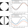 |
Fig. 4 Linearity curve in presence of residuals for unobstructed pupil and toy model pupil. Top left: Unobstructed pupil. Top right: Linearity curve of the petal mode around the residual phase screen for the unobstructed pupil. Bottom left: Obstructed pupil. Bottom right: Linearity curve of the petal mode around the residual phase screen for the toy model pupil. |
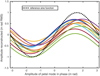 |
Fig. 5 Linearity curve with ten independent residuals with uPyWFS. |
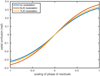 |
Fig. 6 Petal confusion variation with change in phase residual amplitude. |
3.5 Dependence of petal confusion on AO residuals
The first possible origin of this petal confusion comes from the nonlinearity of the uPyWFS. We tested the dependence of the petal confusion on the amplitude of the AO residuals. To do so, we plotted the petal confusion (as the average value of the linearity curve) with respect to the amplitude of the AO residuals. The scaling parameter is a multiplier on the original AO phase residuals. To this end, we used the same residual phase screens as before and scaled them by a multiplicative factor, s ∈ [−1,1]. The dependence curve of c with respect to AO residuals is plotted in Fig. 6 as a function of this scalar. Ten uncorrelated residual realizations were used and the curves of amplitude with scaling were averaged. When s is close to 0 we can write: c(s * ϕ) = s × c(ϕ). The petal confusion is very much a linear effect.
3.6 Origin of the petal confusion
The origin of the petal confusion seems nonetheless to be in the phase residuals. We have found a specific shape that it takes for the PyWFS, but its effects were already reported for the PyWFS and Zernike wavefront sensor by Bertrou-Cantou et al. (2022). Furthermore, it seems to be a linear effect, as was shown by the scalar test. The linearity of the confusion effect means we can construct the phase mode associated with it.
To that end, we computed a map of the confusion, for example how much each individual phase pixel creates petal confusion. As it is a linear effect we can then sum the petal confusion contribution of each pixel into a phase map. For this construction, we put all phase pixels at 0 except one, which was put at 1 rad. We orthogonalized this phase pixel to the petal mode to avoid our reconstruction creating the petal mode. We used this phase as the residual and tested the linearity of the petal mode with this residual. Then we computed the petal confusion caused by this pixel, cx,y. We then plotted the full map of confusion shown in Fig. 7.
This map, which we refer to as a “confusion map,” is expressed in phase space and can be interpreted as the phase mode responsible for the petal confusion. The mode creating petal confusion seems to have two distinct parts: a high-frequency line on each side of the spider (or discontinuity mode), and a low-spatial-frequency sinusoidal phase. This low-order mode comes from the number of modes calibrated in the interaction matrix for the reconstruction of the petal mode. This stems from the petal mode, which can be projected on an infinity of spatial frequencies. The high-frequency signal always appears, even with very high-frequency Zernike integrated in the petalometer interaction matrix. This mode is too high frequency to be controlled by our DM and cannot be separated from the rest of the typical AO residuals. As the petal mode contains high frequency due to its discontinuity, talking about a high frequency being reconstructed as a lower frequency is tricky, but petal confusion (in particular the spider discontinuity component) can be seen as a form of aliasing. It is not a classical aliasing, as over-sampling the phase measurement was tested and doesn’t solve the problem.
The conclusion of the analysis on petal confusion identification is that there will always be some petal confusion that cannot be separated from residuals. Therefore, to measure the petal mode efficiently and to increase the accuracy of the petal mode measurement, we need to reduce the effect of AO residuals.
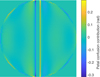 |
Fig. 7 Petal confusion map. |
4 Reducing the impact of residuals on petal mode measurement
To reduce the impact of the residuals on the signal, one solution would be a longer integration time, or moving to a longer wavelength for sensing. This is not compatible with our original aim, which was a fast measurement in the visible, so we need a new strategy to reduce the impact of residuals on the measurement.
4.1 Reducing the effect of residuals in phase space
We now computed the PSD of the atmospheric contribution and the PSD of the petal mode. The residuals’ PSD was computed using the same first-stage system as in part 4, and then their PSFs were averaged over 1000 independent residual phase screens. We can see in Fig. 8 (solid lines) that they have a different distribution in the spatial frequency domain. The PSD of the petal mode was plotted for the same rms amplitude of petal mode as the rms amplitude of residuals (120 nm rms). Residuals have lower PSD values than the petal mode in the low spatial frequencies but dominate in the high spatial frequencies. So if one can filter selectively to keep only the low spatial frequencies, it makes the separation between the petal mode and residuals easier. One can consider the residual as a form of noise on our petal mode measurement. We then want to improve the signal-to-noise (S/N) by selectively filtering the residuals. In the focal plane, there is already this organization by frequency and there is a focal plane already accessible when using a PyWFS: the tip of the PyWFS. We have a new kind of sensor adapted to be a petalometer: a spatially filtered uPyWFS (SF+uPyWFS).
It is to be noted that Usuda et al. (2014) already proposed such a PyWFS for their second WFS channel to lift the λ uncertainty, but with reverse filtering. It was proposed for GMT to filter the low-order frequencies with a chip hiding at the heart of the PSF. When looking at the PSD, the petal mode does indeed evolve differently at higher frequencies than the atmosphere or residuals. Due to the discontinuity in the phase, at high spatial frequencies, the petal mode PSD is over the atmospheric PSD for a comparable amplitude. In terms of petal confusion that would mean a reduction of the low-order part of the petal confusion, so it would be interesting to test it in a further paper.
We simulated the effect of a spatial filter at the tip of the pyramid, as observed from the pupil phase. In this example, we started with the electric field in the entrance pupil plane, propagated it to a focal plane, used a focal plane filter (a circular pinhole), and propagated it to a pupil plane following Fig. 9a.
We then computed the PSD of residuals and petal mode after focal plane filtering (Fig. 8). The pinhole size used for this computation was 5λ/D of the radius.
We see that the first path residuals are suppressed before the petal mode by this focal plane filter. A balance has to be found between reducing the first-stage residual and keeping the spatial filter open to let in as much light as possible. To decide what would be the best size of filter we can think in terms of the S/N. The signal we are interested in is the petal mode. The “noisy signal” comprises the residuals. We computed the variance of the residuals and the variance of the petal mode with a different spatial filter size (SF size).
 (10)
(10)
With our simulation parameter, the 2λ/D spatial filter has the best phase S/N (see Fig. 9). However, having a small SF means limiting the intensity entering the WFS. There is a compromise to find here between the S/N and a loss in intensity. We made the following simulation with a 5λ/D spatial filter. With this spatial filter, we have a S/N of 4 and lose 50% of the intensity. In Fig. 9, curve we see a drop in the S/N starting at 10λ/D. This is due to the residual of the AO (in particular the fitting error), which appears as the intensity at a spatial frequency higher than 10λ/D. In practice, the spatial filter doesn’t filter the AO residuals anymore if it is larger than this radius.
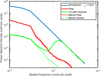 |
Fig. 8 PSD comparison. Atmosphere, first path residual, and petal mode without (plain line) and with 5λ/D filter (dotted line). |
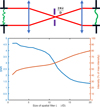 |
Fig. 9 Petal mode to residual ratio for variable spatial filter size. Top: Optical path considered for the spatial filtering test. Bottom: Signal-to-noise ratio for the petal mode and the first path residuals compared to the intensity going through the spatial filter. |
4.2 Effect of the spatial filter on PyWFS signal
A spatially filtered PyWFS (SF+PyWFS) was implemented in the simulation. From a mathematical point of view, a SF+uPyWFS has a phase (uPyWFS) and amplitude mask (SF) in the focal plane. A modulated SF+PyWFS needs the spatial filtering step before the modulation step and is not simply a change of the focal plane mask.
4.3 Effect of spatial filter on linearity curve of PyWFS
The previous linearity test was done using the SF+uPyWFS as the second path petalometer (Fig. 10).
There are two remarkable effects of spatial filtering. The first is less impact on the OGs. As the spatial filter reduces the residuals drastically, the PyWFS is used in a regime closer to the low aberration approximation. Hence, the linearity of the signal improves in the visible here as the OGs are closer to one. Another effect is in the modes impacted by the spatial filter. The sensitivity to the modes drops when the spatial filter radius is under the spatial frequency of the mode. In Fig. 11, we compare the sensitivity of the petal mode, a 3λ/D and 10λ/D sinusoïdal mode, with respect to the spatial filter size. The sensitivity drops fast once the modulation radius is under the spatial frequency of the phase mode. In Fig. 12, we computed the sensitivity of a different SF+uPyWFS compared to the uPyWFS (dark red curve). These two effects make the measurement of the petal mode with a SF+uPyWFS more accurate, as is visible with multiple different residuals in Fig. 13. Compared to Fig. 5, the petal mode reconstruction is closer to the expected sinus reconstruction when using a SF+uPyWFS.
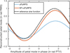 |
Fig. 10 Comparison of the petal mode reconstruction between an uPyWFS and a SF+uPyWFS. |
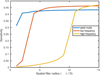 |
Fig. 11 Comparison of the sensitivity of three modes for various spatial filter radii. Low spatial frequency is a 3λ/D sinus and high spatial frequency is a 10λ/D sinus. |
5 Performance on an AO system assisted by a petallometer
Finally, we simulated the full system of the two-path sensor to test the proposed concept of the petalometer as presented in Fig. 3. We compared an uPyWFS and a SF+uPyWFS. The full system was described previously in part 3. The AO first path sensor (a modulated PyWFS) controls the DM (with simple Gaussian continuous influence functions, 20 × 20 actuators), so it creates minioning-type petal residuals. The petalometer commands a hypothetical DM with a pure petal mode as influence function. We subtracted the atmospheric petal mode at frame 0 from the atmospheric phase screen during the whole loop to start from a 0 petal. Measuring the petal with a SF+uPyWFS is equivalent to using the pyramid in a full aperture gain mode (see Plantet et al. 2015). With an optimized sensor, we can at least expect a flux distribution between AO-WFS and petal-WFS of 4000/6: the number of modes used for AO, and the number of petal modes. This would turn into a very small reduction (1/1000th in flux) in terms of the system limit magnitude. On top of this, the characteristic times might be different between the petal mode and the atmosphere mode, depending on their origin. If the petal mode is slow enough (like LWE for instance), its measurement can be averaged with time on a few frames of AO loop, allowing the flux taken for the petalometer path to be reduced further. Since we were using monochromatic PyWFS, the best possible result was to have the petal mode locked at its initial value (zero) during the whole simulation. A bad petalome-ter would not be able to lock the petal mode at a stable value. Furthermore, we added (starting at frame 400 = 0.4 ms of the simulation) a 300 nm rms static petal mode to the atmospheric phase. The aim was to test if our proposed strategy could measure and compensate for the petal mode from other sources than the atmosphere. The parameters were the same as in Table 1 and covered a 1s simulation. The results, in the rms error and projected onto the petal mode, are shown in Figs. 14 and 15, respectively.
The result shows that our continuous influence functions allow the petal mode to stay around zero in the presence of petal flares. The residuals are mostly dominated by the fitting error (dotted red line) with the petal mode on top of it. But if an exterior petal mode is added during the simulation it is not measured and remains uncorrected, as shown by the difference between the green and dotted green line (respectively with and without the 300 nm petal mode jump). The uPyWFS is not a good petalometer: due to the first path residuals it does not measure correctly the petal mode and jumps randomly of 2π petal mode value. We have shown that the SF+uPyWFS can correctly measure the petal mode surrounded by AO residuals, and use this measurement in a correction loop. Moreover, it is able to measure a sudden petal mode jump during the whole simulation. This two-path system allows the AO to stay as close to the fitting error as possible.
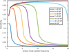 |
Fig. 12 Comparison of sensitivity to pure spatial frequency modes. We see that the SF+uPyWFS has the same sensitivity as the uPyWFS until the spatial frequency is close to the SF radius. |
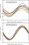 |
Fig. 13 Petal mode reconstruction with 10 independent first path residuals. Comparison between uPyWFS and SF+uPyWFS behavior. The OGs are greatly reduced, as is the petal confusion (reduced by a mean factor of 6). Top: Petal mode reconstruction with ten independent residuals with uPyWFS presented earlier (Fig. 5). Bottom: Petal mode reconstruction with ten independent residuals with SF+uPyWFS. |
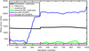 |
Fig. 14 rms error from atmosphere in black, first path AO residuals in green, first path assisted by uPyWFS-petalometer in blue, and first path assisted by SF+uPyWFS-petalometer in magenta. A pure petal mode was added at frame 400 of 300 nm PTV to simulate a petal mode exterior to the atmosphere. We see regular flares of the first path PyWFS, while the SH+uPyWFS helps to keep the residual stable around zero petal during the whole sequence. |
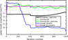 |
Fig. 15 Residual phase of Fig. 14 projected on petal mode. The first path creates visible petal mode residuals as oscillations are between −π and +π. uPyWFS keeps the residual petal closer to 0 petal, but with a jump of −6π (around iteration 250) where it loses its lock on the petal, while SF+uPyWFS stays locked around zero petal. |
6 Conclusion
When the 30 m-class telescopes are completed and take their first scientific images, the petal mode will most certainly be an issue, both for first-light instruments where the LWE is not controlled, and for 2nd generation instruments, in particular those with ExAO where the current petal is unacceptable. This paper proposes a new way of measuring and controlling the petal mode in the loop using visible light. For this aim, we studied a two-path system with one sensor dedicated to atmospheric turbulence measurement and a second one dedicated to the measurement of the petal mode. As a first proposed implementation, we simulated a two-path system using a modulated PyWFS for the atmospheric control and an uPyWFS as the petalometer. We showed that the residuals of the first path still prevent the accurate reconstruction of the petal mode even by an uPyWFS. Another step is needed to accurately reconstruct the petal mode. By analysing the spatial structure of the residuals and the petal mode we showed that a focal plane spatial filter can significantly improve the petal mode reconstruction. After simulation and optimization of the spatial filter size, the spatial filter seemed to greatly improve our reconstruction. With end-to-end simulation we confirmed its interest as a petalometer, precise enough to lock petal mode during the AO loop and capable of measuring unexpected petal flares. The next steps are threefold. First, the spatial-filtering-assisted reconstruction of the petal mode should be tested on bench then on sky using, respectively, the LOOPS bench at Laboratoire d’Astrophysique de Marseille and the PAPYRUS instrument at Observatoire de Haute Provence. Other potential petalometer solutions can be proposed and would surely benefit from the spatial filtering step as well (interferometric measurement with an adapted number of observables). Finally, the solution must also be optimized to a real systems – the proposed SCAO systems of the ELT and the GMT – to prepare for the second generation of instruments.
Acknowledgements
This work benefited from support by the french government under the France 2030 investment plan, as part of the Initiative d’Excellence d’Aix-Marseille Université AMIDEX, program number AMX-22-RE-AB-151, support of the French National Research Agency (ANR) with WOLF (ANR-18-CE31-0018), APPLY (ANR-19-CE31-0011) and LabEx FOCUS (ANR-11-LABX-0013) the Programme Investissement Avenir F-CELT (ANR-21-ESRE-0008), the Action Spécifique Haute Résolution Angulaire (ASHRA) of CNRS/INSU co-funded by CNES, the ECOS-CONYCIT France-Chile cooperation (C20E02), the ORP H2020 Framework Programme of the European Commission’s (Grant number 101004719) and STIC AmSud (21-STIC-09),
References
- Bertrou-Cantou, A. 2021, PhD Thesis, Université de Paris, France [Google Scholar]
- Bertrou-Cantou, A., Gendron, E., Rousset, G., et al. 2020, in Proc. SPIE, 11448, 1144812 [NASA ADS] [Google Scholar]
- Bertrou-Cantou, A., Gendron, E., Rousset, G., et al. 2022, A&A, 658, A49 [NASA ADS] [CrossRef] [EDP Sciences] [Google Scholar]
- Bond, C. Z., Sauvage, J.-F., Schwartz, N., et al. 2022, Proc. SPIE, 12185, 121851B [Google Scholar]
- Bonnefond, S., Tallon, M., Le Louarn, M., & Madec, P.-Y. 2016, Proc. SPIE, 9909, 990972 [NASA ADS] [CrossRef] [Google Scholar]
- Carlomagno, B., Delacroix, C., Absil, O., et al. 2020, J. Astron. Telescopes Rostrum. Syst., 6, 035005 [NASA ADS] [Google Scholar]
- Cayrel, M. 2012, Proc. SPIE, 8444, 84441X [NASA ADS] [CrossRef] [Google Scholar]
- Engler, B., Louarn, M., Vérinaud, C., Weddell, S., & Clare, R. 2022, J. Astron. Telescopes Instrum. Syst., 8, 021502 [NASA ADS] [Google Scholar]
- Esposito, S., Pinna, E., Tozzi, A., Stefanini, P., & Devaney, N. 2003, Proc. SPIE, 5169, 72 [NASA ADS] [CrossRef] [Google Scholar]
- Fauvarque, O. 2017, PhD Thesis, Aix-Marseille, France [Google Scholar]
- Fauvarque, O., Neichel, B., Fusco, T., Sauvage, J. F., & Girault, O. 2016, Optica, 3, 1440 [CrossRef] [Google Scholar]
- Haffert, S. Y., Close, L. M., Hedglen, A. D., et al. 2022, ArXiv e-prints [arXiv:2206.03615] [Google Scholar]
- Hippler, S., Feldt, M., Bertram, T., et al. 2019, Exp. Astron., 47, 65 [NASA ADS] [CrossRef] [Google Scholar]
- Leboulleux, L., Carlotti, A., N’Diaye, M., et al. 2022, Proc. SPIE, 12188, 121881S [Google Scholar]
- Martins, D., Holzlöhner, R., Vérinaud, C., & Kleinclaus, C. 2022, Proc. SPIE, 12187, 1218712 [NASA ADS] [Google Scholar]
- Plantet, C., Meimon, S., Conan, J.-M., & Fusco, T. 2015, Opt. Express, 23, 28619 [NASA ADS] [CrossRef] [Google Scholar]
- Ragazzoni, R. 1996, J. Mod. Opt., 43, 289 [Google Scholar]
- Sauvage, J.-F., Fusco, T., Guesalaga, A., et al. 2015 in Adaptive Optics for Extremely Large Telescopes 4, Conf. Proc., 1 [Google Scholar]
- Schwartz, N., Sauvage, J.-F., Correia, C., et al. 2018a, ArXiv e-prints [arXiv: 1809.08839] [Google Scholar]
- Schwartz, N., Sauvage, J.-F., Correia, C., et al. 2018b, Proc. SPIE, 10703, 1070322 [Google Scholar]
- Usuda, T., Ezaki, Y., Kawaguchi, N., et al. 2014, in Proc. SPIE, 9145, 91452F [NASA ADS] [Google Scholar]
- Vérinaud, C. 2004, Opt. Commun., 233, 27 [Google Scholar]
All Tables
All Figures
|
Fig. 1 Petal mode with variable r0 and spider size. Left: Petal variation for large spiders and variable r0 in first-stage residuals. For spiders larger than the pitch of the ELT DM, the petal mode increases quickly. Right: Petal variation for large spiders and variable r0 in first-stage residuals corrected of the atmospheric turbulence amplitude. |
| In the text | |
|
Fig. 2 Toy model petal mode. |
| In the text | |
|
Fig. 3 2-Path sensor scheme considered. The green path is dedicated to atmosphere wavefront sensing and features a modulated PyWFS and a classical 20×20 actuator DM. The blue path is dedicated to the sensing of the petal mode, features an uPyWFS, and controls only the petal mode of the DM. |
| In the text | |
|
Fig. 4 Linearity curve in presence of residuals for unobstructed pupil and toy model pupil. Top left: Unobstructed pupil. Top right: Linearity curve of the petal mode around the residual phase screen for the unobstructed pupil. Bottom left: Obstructed pupil. Bottom right: Linearity curve of the petal mode around the residual phase screen for the toy model pupil. |
| In the text | |
|
Fig. 5 Linearity curve with ten independent residuals with uPyWFS. |
| In the text | |
|
Fig. 6 Petal confusion variation with change in phase residual amplitude. |
| In the text | |
|
Fig. 7 Petal confusion map. |
| In the text | |
|
Fig. 8 PSD comparison. Atmosphere, first path residual, and petal mode without (plain line) and with 5λ/D filter (dotted line). |
| In the text | |
|
Fig. 9 Petal mode to residual ratio for variable spatial filter size. Top: Optical path considered for the spatial filtering test. Bottom: Signal-to-noise ratio for the petal mode and the first path residuals compared to the intensity going through the spatial filter. |
| In the text | |
|
Fig. 10 Comparison of the petal mode reconstruction between an uPyWFS and a SF+uPyWFS. |
| In the text | |
|
Fig. 11 Comparison of the sensitivity of three modes for various spatial filter radii. Low spatial frequency is a 3λ/D sinus and high spatial frequency is a 10λ/D sinus. |
| In the text | |
|
Fig. 12 Comparison of sensitivity to pure spatial frequency modes. We see that the SF+uPyWFS has the same sensitivity as the uPyWFS until the spatial frequency is close to the SF radius. |
| In the text | |
|
Fig. 13 Petal mode reconstruction with 10 independent first path residuals. Comparison between uPyWFS and SF+uPyWFS behavior. The OGs are greatly reduced, as is the petal confusion (reduced by a mean factor of 6). Top: Petal mode reconstruction with ten independent residuals with uPyWFS presented earlier (Fig. 5). Bottom: Petal mode reconstruction with ten independent residuals with SF+uPyWFS. |
| In the text | |
|
Fig. 14 rms error from atmosphere in black, first path AO residuals in green, first path assisted by uPyWFS-petalometer in blue, and first path assisted by SF+uPyWFS-petalometer in magenta. A pure petal mode was added at frame 400 of 300 nm PTV to simulate a petal mode exterior to the atmosphere. We see regular flares of the first path PyWFS, while the SH+uPyWFS helps to keep the residual stable around zero petal during the whole sequence. |
| In the text | |
|
Fig. 15 Residual phase of Fig. 14 projected on petal mode. The first path creates visible petal mode residuals as oscillations are between −π and +π. uPyWFS keeps the residual petal closer to 0 petal, but with a jump of −6π (around iteration 250) where it loses its lock on the petal, while SF+uPyWFS stays locked around zero petal. |
| In the text | |
Current usage metrics show cumulative count of Article Views (full-text article views including HTML views, PDF and ePub downloads, according to the available data) and Abstracts Views on Vision4Press platform.
Data correspond to usage on the plateform after 2015. The current usage metrics is available 48-96 hours after online publication and is updated daily on week days.
Initial download of the metrics may take a while.