| Issue |
A&A
Volume 680, December 2023
|
|
|---|---|---|
| Article Number | L12 | |
| Number of page(s) | 7 | |
| Section | Letters to the Editor | |
| DOI | https://doi.org/10.1051/0004-6361/202348435 | |
| Published online | 15 December 2023 | |
Letter to the Editor
Bisymmetric pupil modification deconvolution strategy for differential optical transfer function (dOTF) wavefront sensing
1
Université Côte d’Azur, Observatoire de la Côte d’Azur, CNRS, Laboratoire Lagrange, 06304 Nice Cedex, France
e-mail: This email address is being protected from spambots. You need JavaScript enabled to view it.
2
Indian Institute of Astrophysics, II Block Kormangala, Bangalore 560034, India
Received:
30
October
2023
Accepted:
24
November
2023
Abstract
Context. The differential optical transfer function (dOTF) is a model-independent image-based wavefront sensor for measuring the complex pupil field (phase and amplitude). This method is particularly suitable for compensating non-common path aberrations or for the phasing of segmented telescopes that often prevent the so-called diffraction-limit resolution from being achieved with real-world instruments.
Aims. The main problem inherent to the dOTF approach is to address the effect of the convolution. The resolution of the recovered complex pupil field is impacted by the size of the pupil modification. The complex pupil field estimated by the dOTF is blurred by convolution with the complex conjugate of the pupil modification. If the pupil modification involves a non-negligible region of the pupil (actuator or segment poke), it causes significant blurring and resolution loss.
Methods. We propose a bisymmetric pupil modification deconvolution strategy to solve this problem. We use two different dOTFs with the opposite-sign pupil modification to identify the pupil modification location and four dOTFs with a symmetric pupil modification to complete the knowledge of their impact on the complex pupil field prior to the deconvolution process in the Fourier domain. The proposed strategy solves the intrinsic limitation of a former deconvolution algorithm, namely the cross-iteration deconvolution algorithm, which is restricted to amplitude pupil modification and precludes its applicability to phase pupil modification.
Results. The bissymetric pupil modification deconvolution strategy is a novel probing pattern that permits the extension of iterative cross-deconvolution to phase-only probes. The effectiveness of the proposed approach has been validated analytically and with numerical simulations.
Conclusions. The bisymmetric pupil modification deconvolution strategy can improve the resolution and accuracy of dOTF wavefront sensing and contributes to efficient and precise image-based wavefront sensing techniques.
Key words: instrumentation: adaptive optics / instrumentation: high angular resolution / techniques: high angular resolution / telescopes
© The Authors 2023
 Open Access article, published by EDP Sciences, under the terms of the Creative Commons Attribution License (https://creativecommons.org/licenses/by/4.0), which permits unrestricted use, distribution, and reproduction in any medium, provided the original work is properly cited.
This article is published in open access under the Subscribe to Open model. This email address is being protected from spambots. You need JavaScript enabled to view it. to support open access publication.
1. Introduction
Maintaining an almost aberration-free wavefront over time for any coronagraphic instrument used in high-contrast imaging is a must, but is very challenging in practice because of aberrations. This goal requires a high level of wavefront control, which involves correcting for dynamical, quasi-static, and static aberrations. This is the so-called speckle noise. To address these challenges, various wavefront sensors have been developed and proposed for applications such as adaptive optics, active optics for telescopes and instruments, and cophasing optics.
The differential optical transfer function (Codona 2013; Codona & Doble 2015, dOTF) is a phase-retrieval technique used to estimate the complex field of an optical system. Unlike some other phase-retrieval methods, such as Gerchberg–Saxton (Gerchberg 1972), phase diversity (Mugnier et al. 2006), fast and furious (Korkiakoski et al. 2014), or parametric phase retrieval (Brady et al. 2018), dOTF is model independent and entirely empirical. The dOTF technique features various advantages: (i) It does not rely on a prior model of the optical system, which can be challenging to obtain accurately; (ii) it works by comparing two differential images of the optical transfer function (OTF, which describes the system’s ability to transfer spatial frequencies from the object to the image) taken in the focal plane of the imaging system; (iii) unlike some other phase-retrieval techniques that require iterative algorithms to converge to a solution, dOTF is a single-step, open-loop method. It provides an estimate of the electric field of the entire pupil with as few as three images. It can be advantageous in situations where speed and simplicity are expected.
A fundamental challenge in the dOTF method is the trade-off between the signal-to-noise ratio (S/N) of the dOTF and the resolution of the recovered complex pupil field. This trade-off occurs because of the convolution of the complex pupil field with the complex conjugate of the pupil modification. Involving a small portion of the pupil in the modification provides a high-resolution image of the pupil field, but with a weaker signal. Alternatively, involving a large portion of the pupil in the modification provides a low-resolution image of the pupil field, but with a higher signal. In particular, when the dOTF method is used to sense the phasing error of a segmented telescope, pupil modification can be introduced by blocking one segment near the edge of the pupil. The recovered phase is significantly blurred, and the resolution of the recovered phase is significantly decreased. While deconvolution can potentially improve the resolution of the recovered phase in dOTF applications, it requires precise knowledge of the complex pupil modification and location, which is challenging to obtain in practical scenarios. Even if a known phase change with a known piston (or tip-tilt) change of a pupil region is introduced, the exact nature of the complex pupil modification remains uncertain. This limitation underscores the complexity and practical considerations associated with using dOTF in applications such as segmented telescope phasing error sensing or non-common path aberrations (NCPA) correction. The bisymmetric pupil modification deconvolution strategy proposes a solution to this problem.
The paper is structured as follows: in Sect. 2 we briefly recall the principle of the dOTF wavefront sensor, signal properties, and sequence options, and discuss practical limitations. In Sect. 3 we explain the bisymmetric pupil modification strategy in detail. Section 4 concludes with the efficiency of the technique.
2. Differential optical transfer function
2.1. Principle and conventions
In this section, we briefly recall the principle of the dOTF and the notation conventions we used, which are described in Fig. 1. We note ψ as the product of the incident electric field ψ0 and the pupil transmission mask function M. For convenience, pupil plane and focal plane variables are omitted in the following. The Fourier transform of a function f is noted ℱ(f), and the inverse Fourier transform is expressed as ℱ−1(f). The asterisk means the complex conjugate, the cross denotes the product operator, and the crossed circle denotes the convolution product. The pupil transmission function M can be altered when applying a dOTF probe (i.e., a pupil modification), as in Codona (2013), so that M is transformed into M + δM (see Fig. 1). For the sake of simplicity, Ψ and δΨ are the Fourier transforms of ψ and δψ. For a deeper understanding of the dOTF method, we refer to the full treatment in the original paper from Codona (2013) or other relevant references (Codona 2012; Codona & Doble 2015).
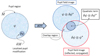 |
Fig. 1. Generic pupil with a pupil modification near the edge of the pupil (left), and conceptual drawing of the dOTF contents and location relative to the introduced pupil modification (right). |
The dOTF wavefront sensor is a noninterferometric, noniterative method for estimating the complex amplitude field (amplitude and phase) in the pupil of an optical imaging system, without requiring any specialized hardware or sophisticated postprocessing techniques. dOTF works by comparing two differential images of the optical transfer function (OTF) of the imaging system. The OTF, denoted 𝒪, can be expressed as the autocorrelation of the pupil field ψ. Differential images are taken in the focal plane of the system, where for one of the images, a pupil modification is introduced. The pupil modification can be in phase or amplitude, or both. Because deformable mirrors are routinely used in high-contrast imaging, pupil modification can be implemented by an actuator or segment poke in a straightforward way.
The dOTF, denoted δ𝒪, can be given by
 (1)
(1)
Equation (1) can further be rewritten as
 (2)
(2)
Equation (2) shows that the dOTF includes three terms that are represented in the right part of the conceptual design shown in Fig. 1. Each term is a correlation between two field factors, either the unmodified pupil field (ψ), or the pupil modification (δψ). The first term corresponds to the field in the pupil region that is convolved by the pupil modification. The second term corresponds to the conjugated copy of the first term, reflected about the origin. It provides redundant information. The last term is the quadratic term where these two first terms overlap at the location of the pupil modification and are related to the autoconvolution of the pupil modification. The first and second terms include a region of overlap between the two pupil regions that depends on the placement of the pupil modification. A cartoon example of the form of the dOTF is given for a pupil modification localized to the edge of the pupil in Fig. 1.
Equation (2) shows that a smaller pupil modification area can lead to a higher resolution in the recovered wavefront phase map by reducing the blurring effect associated with cross correlation. However, this choice may also depend on the specific application, the level of detail required, and the trade-offs between modification size and other factors. Equation (2) also shows that a complete measurement of ψ (over the whole pupil) requires two dOTFs with different pupil modifications. Because we lose information in the pupil modification region, we need to combine two dOTFs with different pupil modification locations in order to build up a complete measurement of the electric field across the entire pupil.
2.2. Alternative implementation
As shown by Eq. (1), the original implementation of dOTF takes a difference between an OTF image with a pupil modification and an OTF image without any pupil modifications. An alternative implementation proposed by Nguyen et al. (2023) takes a difference between an OTF image with a pupil modification and an OTF image with the opposite sign of pupil modification. This implementation conceptually refers to pair-wise probing wavefront-sensing techniques (Give’on et al. 2007) (see Appendix E for a brief discussion) and is expressed as
 (3)
(3)
Equation (3) can further be rewritten as
![Mathematical equation: $$ \begin{aligned} \delta \mathcal{O} = 2 \times \left[ \psi \otimes \delta \psi ^{*} + \delta \psi \otimes \psi ^{*} \right], \end{aligned} $$](/articles/aa/full_html/2023/12/aa48435-23/aa48435-23-eq4.gif) (4)
(4)
where taking a difference of a positive- and negative-sign pupil modification, the quadratic terms of Eq. (2) cancel, leaving just the two cross terms, whose magnitudes are doubled. Because the overlap region of the quadratic term cancels, it provides valuable information on the pupil modification location in the dOTF: We can extract both pupil modification location and dimension from this missing term, which will appear obscure in the image. This property (illustrated in Appendix A, Fig. A.1) is used as a first calibration step in our deconvolution strategy for a set of symmetric pokes (diametrically opposite pokes).
We note that the quadratic term size is double the pupil modification size because of the convolution process.
2.3. Deblurring the dOTF
In both the original (Eq. (2)) and alternative implementation (Eq. (4)), the pupil field is blurred by convolution with the complex conjugate of the pupil modification. A comparison between the original phase and the recovered phase using dOTF demonstrates that the recovered phase is blurred, resulting in a significant reduction in resolution (see Appendix C). A solution for the problem involves a deconvolution algorithm that can improve the resolution and accuracy of wavefront-phase maps. However, it is contingent on accurate knowledge of the complex pupil modification, which is often elusive in practical situations (Knight et al. 2015).
A recent deconvolution strategy has been proposed by Jiang et al. (2019) and is referred to as the cross-iteration deconvolution algorithm. The cross-iteration strategy is proposed for the deconvolution of the dOTF (i.e., δ𝒪1) using an additional dOTF (δ𝒪2), which corresponds to a different pupil modification and localization. In this scheme, the two different dOTFs provide two estimated pupil fields with different regions of overlap. The first dOTF can be expressed as
 (5)
(5)
and the second dOTF as
 (6)
(6)
where δψ1 and δψ2 are the two different pupil field modifications. In the cross-iterative deconvolution process, and because the modification is obtained by blocking/occulting a small area of the pupil, the estimate of the pupil modification (δψ1) is directly obtained from δ𝒪2 in its corresponding pupil subdomain (see Eq. (3) of Jiang et al. 2019). The deconvolution of δ𝒪1 is performed with δψ1 estimated in the Fourier space, using Fourier transformation,
 (7)
(7)
Equation (7) can be written as
 (8)
(8)
Then inverse Fourier transform is further performed to obtain
 (9)
(9)
Equation (9) shows that in the first term, the pupil field ψ is no longer blurred by convolution with the complex conjugate of the pupil modification. Because the accuracy of the estimate δψ1 is affected by the convolution inherent in the second dOTF, the performance of the deconvolution has to be improved iteratively, and thus Eq. (9) provides an estimator of ψ that needs to be refined iteratively. However, a drawback of this strategy is that it precludes the use of phase modification in the pupil. According to Jiang et al. (2019), the technique can only work when the amplitude pupil modification (pupil blockage) satisfies Eq. (3) of that paper. The complex field of pupil modification is defined as the difference between the modified pupil field after blocking and the unmodified field. In this context, the complex field of modification represents the opposite of the unmodified pupil field in the area of modification in a straightforward way (Jiang et al. 2019, Eqs. (3) and (11)). This underlying prior knowledge when pupil blockage is used to introduce pupil modification has no equivalent when phase pupil modification is involved. In addition, we note that in the cross-iteration deconvolution algorithm, the third term in Eq. (9), the quadratic term from Eq. (5), remains.
3. Bisymmetric pupil modification strategy
We propose a novel deconvolution strategy that ends the limitation of the cross-iteration deconvolution algorithm. This then allows a precise and accurate estimate of the complex pupil modification ( or equivalently
  ) that is required for an efficient deconvolution (see Eq. (8)) when phase modification is involved (segment or actuator poke). Our approach is indeed independent of the pupil modification type (amplitude or phase).
The basic principle of the algorithm is described in the flow diagram presented in Fig. 2. Step 1 represents a calibration step in which two sets of dOTF are produced, namely  and
and  . The first set corresponds to the difference between an OTF image with a pupil modification (+δM0) and an OTF image with the opposite-sign pupil modification (−δM0). The second set is identical, but involves a symmetric segment or actuator that is diametrically opposite (denoted
  ) to that of the first dOTF. In Appendix A, Fig. A.1 presents a conceptual drawing of this step. These two dOTFs can be written as
 (10)
(10)
 (11)
(11)
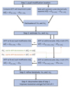 |
Fig. 2. Flow diagram of the bisymetric pupil modification deconvolution strategy for the dOTF wavefront sensing. |
This first set of dOTFs reveals the precise location of δψ0 and  because the quadratic term in the dOTF cancels. In addition, the magnitude of the first term in the dOTF is doubled, and a full field of ψ can later be estimated because δM0 and
  are different (symmetric over the pupil).
Steps 2 and step 3 are fundamentally equivalent to the whole architecture procedure as proposed by Jiang et al. (2019), but instead of relying on two dOTFs, it requires four dOTFs to adapt for phase pupil modification (see Appendix D). Two sets of two dOTFs are produced. Each set of two dOTFs provides an estimate of the pupil field with different regions of overlap. The first set of dOTFs ( and
and  ), defined as
 (12)
(12)
and
 (13)
(13)
intends to provide a first estimate of the pupil field modification ( , because the subtraction of
  by
by  allows calibration of the impact of
  ) used in the second set for deconvolution according to Eq. (9). Therefore, the first stage of step 2 is to estimate the second complex pupil modification, which can be used for the deconvolution of the second set of dOTFs. From the second set of dOTFs (
 and
and  ), defined as
 (14)
(14)
and
 (15)
(15)
an estimate of δψ0 used for deconvolution of the first set of dOTFs is possible. In Appendix B, Fig. B.1 presents a conceptual drawing of step 2. Because the accuracy of  is affected by the convolution inherent in the first set of dOTF and results in a blurring effect, the performance of the deconvolution of the second set of dOTFs is restricted. However, we can improve the performance of the deconvolution in a cross-iteration manner as proposed in Jiang et al. (2019). This is the purpose of step 3, described in Fig. 2, which illustrates the iterative nature of the deconvolution process. The iterative procedure is deterministic.
Finally, when the optimal performance in the deconvolution process of all sets of dOTFs is reached, so that optimal estimates of  and δψ0 are obtained, they can be applied to deconvolve data from step 1, providing an estimate of ψ over a full field and with an improved resolution. This corresponds to step 4 in the flow diagram presented in Fig. 2. In Appendix C, a demonstration of phasing optics is provided to illustrate the efficiency of the algorithm (here restricted to steps 2 and 3, which are the heart of the strategy, and because in the simulation, step 1 is unnecessary).
4. Conclusion
The dOTF offers a practical and model-independent approach that can work in various imaging scenarios, particularly when there is a need for a rapid and straightforward solution. The bisymmetric pupil modification deconvolution strategy ends the limitation of the cross-iteration deconvolution algorithm and allows an efficient deconvolution when phase pupil modification (actuator or segment poke) is used in the dOTF process. By introducing a controllable phase pupil modification, such as actuating a telescope or instrument deformable mirror segment or actuator in a piston (or tip-tilt) to make the dOTF measurement, we propose a procedure for increasing the resolution along with an increase in the S/N. Because deformable mirrors of various kinds are routinely used on most telescopes today or on high-contrast imaging instruments, the segment or actuator poke can be used for dOTF in a straightforward way. When pupil blockage is selected (amplitude pupil modification instead of phase pupil modification), we note that the cross-iteration deconvolution strategy proposed by Jiang et al. (2019) corresponds to a particular and simplified case of our general strategy.
Acknowledgments
The authors acknowledge the financial support from the scientific council de l’Observatoire de la Côte d’Azur under its strategic scientific program.
References
- Ahn, K., Guyon, O., Lozi, J., et al. 2023, A&A, 673, A29 [NASA ADS] [CrossRef] [EDP Sciences] [Google Scholar]
- Brady, G. R., Moriarty, C., Petrone, P., et al. 2018, in SPIE Astronomical Telescopes + Instrumentation (Austin: SPIE) [Google Scholar]
- Codona, J. 2012, Proceedings Adaptive Optics Systems III, 8447, 84476P [NASA ADS] [CrossRef] [Google Scholar]
- Codona, J. L. 2013, Opt. Eng., 52, 097105 [CrossRef] [Google Scholar]
- Codona, J. L., & Doble, N. 2015, J. Astron. Telesc. Instrum. Syst., 1, 029001 [NASA ADS] [CrossRef] [Google Scholar]
- Gerchberg, R. W. 1972, Optik, 35, 237 [Google Scholar]
- Give’on, A., Kern, B., Shaklan, S., Moody, D. C., & Pueyo, L. 2007, in Astronomical Adaptive Optics Systems and Applications III, eds. R. K. Tyson, & M. Lloyd-Hart, SPIE Conf. Ser., 6691, 66910A [Google Scholar]
- Haffert, S. Y., Males, J. R., Ahn, K., et al. 2023, A&A, 673, A28 [NASA ADS] [CrossRef] [EDP Sciences] [Google Scholar]
- Jiang, F., Ju, G., Qi, X., & Xu, S. 2019, Opt. Lett., 44, 4283 [NASA ADS] [CrossRef] [Google Scholar]
- Knight, J. M., Rodack, A. T., Codona, J. L., Miller, K. L., & Guyon, O. 2015, in Techniques and Instrumentation for Detection of Exoplanets VII, ed. S. Shaklan, SPIE Conf. Ser., 9605, 960529 [NASA ADS] [CrossRef] [Google Scholar]
- Korkiakoski, V., Keller, C. U., Doelman, N., et al. 2014, Appl. Opt., 53, 4565 [NASA ADS] [CrossRef] [Google Scholar]
- Mugnier, L. M., Blanc, A., & Idier, J. 2006, Advances in Imaging and Electron Physics (Elsevier), P. Hawkes, 141, 1 [CrossRef] [Google Scholar]
- Nguyen, M. M., Por, E. H., Sahoo, A., et al. 2023, in Techniques and Instrumentation for Detection of Exoplanets XI, SPIE, 12680, 834 [Google Scholar]
Appendix A: Illustration of step 1
A conceptual drawing illustrating step 1 of the bisymmetric pupil modification deconvolution algorithm is presented in Fig. A.1. Generic pupils are presented in the left part of the drawing, and the right part presents the resulting sketch of the corresponding dOTF. In Fig. A.1, two situations are presented: (i) A dOTF, namely  , is obtained from the difference between an OTF image with a pupil modification (δM0) and an OTF image with the opposite-sign pupil modification; (ii) a second dOTF, namely
  , is obtained from the difference between an OTF image with another pupil modification (
 ) different from δM0, and an OTF image with the opposite-sign pupil modification, where
  is the symmetric about the origin of δM0. In both dOTFs, the quadratic term of Eq. 2 or 5 and 6 cancels and leaves an empty space (arbitrarily expressed in white) in the drawing, corresponding to a region in which the values are nearly zero. The size of the cancelled region is twice the size of the pupil modification field δψ0 or
  . This first step 1 allows an accurate identification of the location of the δψ0 or
  terms that are required further in the whole algorithm for deconvolution aspects.
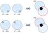 |
Fig. A.1. Conceptual drawing representing step 1 of the flow diagram in Fig. 2. Left: Generic situation in which a pupil modification near the edge of the pupil is performed, with the opposite-sign pupil modification between the pupil image and with a diametrically symmetric pupil modification (top/bottom). Right: Corresponding dOTF in which all terms involved are located relative to the pupil modification. The part that is reflected about the origin (red) and the conjugated part of the pupil field image (blue) are also shown. |
Appendix B: Step 2 illustration
A conceptual drawing illustrating step 2 of the bisymmetric pupil modification deconvolution algorithm, involving four dOTFs, is presented in Fig. B.1. Generic pupils are presented in the left part of the drawing, and the right part presents the resulting sketch of the corresponding dOTF. From a practical point of view, dOTFs operate as pairs of dOTFs. Both  and
and  are required to estimate the contribution of
  (illustrated by a circle with a blue-and-white checkerboard pattern in the top left corner of
  ), corresponding to the
  pupil modification term.
  corresponds to a classical dOTF form when
  includes a common segment or actuator poke term in the two OTF images for calibration purposes. Similarly, both
  and
and  are required to estimate the δψ0 (illustrated by a circle with a blue-and-white checkerboard pattern in the right bottom corner of
  ) contribution corresponding to the δM0 pupil modification term.
  corresponds to a classical dOTF form when
  includes a common segment or actuator poke term in the OTF images for calibration purposes.
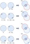 |
Fig. B.1. Conceptual drawing representing step 2 of the flow diagram in Fig. 2. Left: Generic pupil where the pupil modification near the edge of the pupil is presented. Right: Corresponding dOTF. The part that is reflected about the origin (red) and the conjugated part of the pupil field image (blue) are also shown. |
Appendix C: Cophasing optics demonstration
The selection of the size of the modification area in the pupil is a delicate balance between obtaining high spatial resolution and maintaining a strong signal against image noise. Practical considerations often lead to a compromise, where a larger modification area is chosen to enhance the S/N, even though it results in a decrease in the resolution of the recovered wavefront phase map. Nonetheless, in the scenario involving the use of dOTF to sense the phasing error of a segmented telescope, pupil modification is introduced by blocking or poking one segment near the edge of the pupil. A cophasing operation is presented with numerical simulations to demonstrate that the bisymmetric pupil modification deconvolution algorithm works as expected. The simulations assumed a segmented hexagonal telescope composed of 37 segments over four hexagonal rings without central obscuration or secondary mirror supports. The simulations used simple Fraunhofer propagators between the pupil and image planes that were implemented as fast Fourier transforms (FFTs) generated with a Python code. The matrices were 1024 × 1024 pixels in size, and the focal plane sampling was about 4 pixels per λ/D, where D is the entrance pupil diameter. No dynamical aberrations were included, and the system was free of aberrations with a spatial frequency that was lower than the segment size was large. Monochromatic light with a wavelength λ = 632 nm was used. The simulations were noise free and made for illustration purposes alone. All segment pokes involved in dOTFs were λ/4 segment mechanical displacements, as proposed in Codona (2013). We independently analyzed the convergence and efficiency of the deconvolution algorithm as well as the residual RMS in two cases: first with piston alone, and then with both piston and tip-tilt errors. The simulations assumed random piston and tip/tilt errors following a normal distribution over the pupil with an initial RMS of 105 nm (piston alone, λ/6 RMS) and 72 nm (piston and tip/tilt, ∼λ/9 RMS, with equal RMS distribution for all aberrations). Figure C.1 shows the result of dOTF wavefront sensing without deconvolution that is readily affected by the blurring effect (left image), with the proposed bisymmetric pupil modification deconvolution algorithm after iteration 1 (middle image), and similarly, after iteration 5 (right image) for the piston-only scenario. Figure C.2 shows similar results for the simulation involving both piston and tip/tilt errors. We can see the resolution improvement and that the proposed approach is effective. Figure C.3 shows the error in piston measurement (for the piston-only scenario) between the recovered phase and the original phase during the bisymmetric pupil modification deconvolution process as a function of the segment number. The blue dots represent data without deconvolution, and the orange, green, red, and purple dots after iterations 1, 2, 3, and 4 of the deconvolution algorithm.
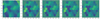 |
Fig. C.1. Results of the bisymmetric pupil modification deconvolution algorithm with piston only (λ/6 nm RMS). The first image on the left shows the original phasing error of a segmented pupil with the blurring effect. From left to right, the images show the intermediate result of the dOTF phase during the algorithm process from the first to the fourth iteration. The corresponding quantitative results are presented in Fig. C.3. |
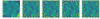 |
Fig. C.2. Results of the bisymmetric pupil modification deconvolution algorithm with piston and tip/tilt errors (λ/9 nm RMS). The first image on the left shows the original phasing error of a segmented pupil with the blurring effect. From left to right, the images show the intermediate result of dOTF phase during the algorithm process from the first to the fourth iteration. The corresponding quantitative results are presented in Fig. C.4. |
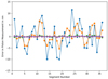 |
Fig. C.3. Measured error in piston (piston-only scenario) between the recovered phase and the original phase during the bisymmetric pupil modification deconvolution process as a function of the segment number. The blue, orange, green, red and purple dots correspond to the situation without deconvolution and with deconvolution after iterations 1, 2, 3, and 4. |
The dispersion in the data is greatly and rapidly reduced with the deconvolution process. Figure C.4 presents the same error in the piston (left plot) and tip/tilt (middle and right plots) measurement in the case of piston and tip/tilt errors. In the piston and tip/tilt scenario, while without deconvolution of the RMS (blue) error in piston is 12 nm and ∼ 35 nm for tip/tilt, it reduces at iteration 4 (purple) of the proposed algorithm to 1.5 nm (piston) and 4 nm (tip/tilt).
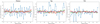 |
Fig. C.4. Results of the bisymmetric pupil modification deconvolution algorithm with piston and tip/tilt errors (λ/9 nm RMS). From left to right: Error in measurement of piston, tip, and tilt. |
Appendix D: Phase pupil modification
When using the dOTF with noncompact phase pupil modification (e.g., segment or actuator poke), and even when we have a good idea of how much we move a test segment or actuator, the introduced phase change is not entirely known. Even if the phase change by poking an actuator or segment is known, the modification of the complex field at the actuator or segment location remains unknown. This is particularly true for the segment poke, where the initial piston and tip/tilt alignment are unknown and not ideal. We can model the situation, following the Nguyen et al. (2023) formalism to consider in the dOTF the effect of the environmental drifts, by adding an additional delta term (ΔM) to the pupil modification (δM), where ΔM < δM. In this situation, the dOTF is modified from the original expression
 (D.1)
(D.1)
to the following expression:
 (D.2)
(D.2)
Equation D.2 can be rewritten as
 (D.3)
(D.3)
After distribution and simplification, Eq. D.3 can further be rewritten as
 (D.4)
(D.4)
where δ𝒪0 is the original dOTF. Equation D.4 shows two additional terms, where δψ ⊗ Δψ* belongs to the reflected and conjugated pupil field image and Δψ ⊗ δψ* belongs to the pupil field image. When redundant information (selecting only pupil field image terms) is omitted, Eq. D.4 can be simplified or restricted to
 (D.5)
(D.5)
Equation D.5 shows that the estimate of the electric field is subject to a phase offset corresponding to the unknown phase present at the poke location. The result emphasizes the need of calibrating dOTF images to remove the global piston and tip/tilt aberrations in phase when outer pupil segment is used for dOTF. Because poking an actuator instead of a segment cannot be considered an idealized Dirac but Gaussian poke, the reasoning still applies. While the offset is small in principle, segment poke may introduce significant segment piston or tip/tilt error (misalignment) in addition to other types of wavefront errors. Either way, segment or actuator pokes, the resulting phase pupil modification reduces the resolution and adds an additional phase term to the dOTF.
Appendix E: Controlling amplitude and phase
In pair-wise probing (PWP), phase probes are added to the deformable mirror (DM) to modulate the focal plane speckles to reconstruct the full electric field. PWP make the use of several phase offsets of the probe as well as a sign change of the phase probe. This sensing method is commonly combined with electric field conjugation (EFC, Give’on et al. 2007)), which cancels the electric field in the focal plane by injecting equal-strength speckles with an opposite phase. The recently proposed implicit electric field conjugation (iEFC, Haffert et al. 2023) is a model-independent version of EFC and it can be empirically calibrated by a probing-the-probe technique used for self-calibration of the electric field probes applied (Haffert et al. 2023; Ahn et al. 2023). In this context, iEFC and dOTF share important similarities that may suggest they may be one and the same, just one Fourier transform away from each other: (i) both techniques are model-independent, (ii) the complete electric field is measured or can be measured by adding phase probes on the DM, (iii) both techniques make the use of self-estimation of the probes, and (iv) both techniques rely on difference of images: iEFC assumes a linear response between the DM commands and the differential images from PWP, while the dOTF relies on the differential OTFs, where the difference of numerical Fourier transform of images is equivalent to performing the numerical Fourier transform of the difference of the images.
All Figures
|
Fig. 1. Generic pupil with a pupil modification near the edge of the pupil (left), and conceptual drawing of the dOTF contents and location relative to the introduced pupil modification (right). |
| In the text | |
|
Fig. 2. Flow diagram of the bisymetric pupil modification deconvolution strategy for the dOTF wavefront sensing. |
| In the text | |
|
Fig. A.1. Conceptual drawing representing step 1 of the flow diagram in Fig. 2. Left: Generic situation in which a pupil modification near the edge of the pupil is performed, with the opposite-sign pupil modification between the pupil image and with a diametrically symmetric pupil modification (top/bottom). Right: Corresponding dOTF in which all terms involved are located relative to the pupil modification. The part that is reflected about the origin (red) and the conjugated part of the pupil field image (blue) are also shown. |
| In the text | |
|
Fig. B.1. Conceptual drawing representing step 2 of the flow diagram in Fig. 2. Left: Generic pupil where the pupil modification near the edge of the pupil is presented. Right: Corresponding dOTF. The part that is reflected about the origin (red) and the conjugated part of the pupil field image (blue) are also shown. |
| In the text | |
|
Fig. C.1. Results of the bisymmetric pupil modification deconvolution algorithm with piston only (λ/6 nm RMS). The first image on the left shows the original phasing error of a segmented pupil with the blurring effect. From left to right, the images show the intermediate result of the dOTF phase during the algorithm process from the first to the fourth iteration. The corresponding quantitative results are presented in Fig. C.3. |
| In the text | |
|
Fig. C.2. Results of the bisymmetric pupil modification deconvolution algorithm with piston and tip/tilt errors (λ/9 nm RMS). The first image on the left shows the original phasing error of a segmented pupil with the blurring effect. From left to right, the images show the intermediate result of dOTF phase during the algorithm process from the first to the fourth iteration. The corresponding quantitative results are presented in Fig. C.4. |
| In the text | |
|
Fig. C.3. Measured error in piston (piston-only scenario) between the recovered phase and the original phase during the bisymmetric pupil modification deconvolution process as a function of the segment number. The blue, orange, green, red and purple dots correspond to the situation without deconvolution and with deconvolution after iterations 1, 2, 3, and 4. |
| In the text | |
|
Fig. C.4. Results of the bisymmetric pupil modification deconvolution algorithm with piston and tip/tilt errors (λ/9 nm RMS). From left to right: Error in measurement of piston, tip, and tilt. |
| In the text | |
Current usage metrics show cumulative count of Article Views (full-text article views including HTML views, PDF and ePub downloads, according to the available data) and Abstracts Views on Vision4Press platform.
Data correspond to usage on the plateform after 2015. The current usage metrics is available 48-96 hours after online publication and is updated daily on week days.
Initial download of the metrics may take a while.