| Issue |
A&A
Volume 680, December 2023
|
|
|---|---|---|
| Article Number | A46 | |
| Number of page(s) | 14 | |
| Section | Astrophysical processes | |
| DOI | https://doi.org/10.1051/0004-6361/202347647 | |
| Published online | 12 December 2023 | |
Linear stability analysis of relativistic magnetized jets
The Kelvin-Helmholtz mode
Department of Physics, National and Kapodistrian University of Athens, University Campus, Zografos, 157 84 Athens, Greece
e-mail: This email address is being protected from spambots. You need JavaScript enabled to view it.
; This email address is being protected from spambots. You need JavaScript enabled to view it.
Received:
3
August
2023
Accepted:
8
September
2023
Abstract
Aims. We study the stability properties of relativistic magnetized astrophysical jets in the linear regime. We consider cylindrical cold jet configurations with constant Lorentz factor and constant density profiles across the jet. We are interested in probing the properties of the instabilities and identifying the physical quantities that affect the stability profile of the outflows.
Methods. We conducted a linear stability analysis on the unperturbed outflow configurations we are interested in. We focus on the unstable branches, which can disrupt the initial outflow. We proceeded with a parametric study regarding the Lorentz factor, the ratio of the rest mass density of the jet to that of the environment, the magnetization, and the ratio of the poloidal component of the magnetic field to its toroidal counterpart measured on the boundary of the jet. We also consider two choices for the pressure of the environment, either thermal or magnetic, and check if this choice affects the results. Additionally, we applied a WKBJ method at the radius of the jet in order to study the local stability properties. Finally, we adapted the jet configuration in Cartesian geometry and compared the planar flow results with the results of the cylindrical counterpart.
Results. While investigating the stability properties of the configurations, we observed the existence of a specific solution branch, which showcases the growth timescale of the instability comparable to the light crossing time of the jet radius. Our analysis focuses on this solution. All of the quantities considered for the parametric study affect the behavior of the mode while the magnetized environments seem to hinder its development compared to the hydrodynamic equivalent. Also, our analysis of the eigenfunctions of the system alongside the WKBJ results show that the mode develops in a very narrow layer near the boundary of the jet, establishing the notion of locality for the specific solution. The results indicate that the mode is a relativistic generalization of the Kelvin-Helmholtz instability. We compare this mode with the corresponding solution in Cartesian geometry and define the prerequisites for the Cartesian Kelvin-Helmholtz to successfully approximate the cylindrical counterpart.
Conclusions. We identify the Kelvin-Helmholtz instability for a cold nonrotating relativistic jet carrying a helical magnetic field. Our parametric study reveals the important physical quantities that affect the stability profile of the outflow and their respective value ranges for which the instability is active. The Kelvin-Helmholtz mode and its stability properties are characterized by the locality of the solutions, the value of the angle between the magnetic field and the wavevector, the linear dependence between the mode’s growth rate and the wavevector, and finally the stabilization of the mode for flows that are ultrafast magnetosonic. The cylindrical mode can be approximated successfully by the Cartesian Kelvin-Helmholtz instability whenever certain length scales are much larger than the jet radius.
Key words: instabilities / magnetohydrodynamics (MHD) / methods: analytical / ISM: jets and outflows / galaxies: jets / relativistic processes
© The Authors 2023
 Open Access article, published by EDP Sciences, under the terms of the Creative Commons Attribution License (https://creativecommons.org/licenses/by/4.0), which permits unrestricted use, distribution, and reproduction in any medium, provided the original work is properly cited.
This article is published in open access under the Subscribe to Open model. This email address is being protected from spambots. You need JavaScript enabled to view it. to support open access publication.
1. Introduction
Jets are collimated plasma outflows that are most often created by the accretion of matter onto a massive cosmic object. The first ever observed jet was that of M87 (Curtis 1918). Since then, many such cosmic outflows have been discovered and many have been thoroughly studied. The central engine properties of these jets may vary greatly in terms of physical parameters. There are outflows generated by protostars (young stellar objects; YSOs), supermassive black holes (in active galactic nuclei; AGN), and stellar mass black holes (in gamma ray bursts; GRBs), and binary systems (systems of dual black holes or a black hole and a companion star in X-ray binaries; XRBs).
The most plausible launching mechanism requires an accretion disk threaded by a vertical magnetic field. Due to the rotation of the black hole or the disk, a toroidal magnetic field component is created that launches the outflow. In the literature, this magnetic launching scenario was analyzed for example in the seminal publications of Blandford & Znajek (1977) and Blandford & Payne (1982). The jet launching mechanism consists of many subprocesses, which are studied independently in numerous publications. There are works studying the feeding process to the central object, the acceleration and collimation processes, and finally the properties and dynamics of jets at various length scales.
In the present study, we focus mainly on mildly relativistic jets. These outflows have a typical bulk Lorentz factor of ∼2 − 5 and lengths that span from ∼100 pc up to ∼1 kpc; a typical example of such an outflow could be an AGN jet. These scales imply enhanced stability properties, as the ratio of the total length of a jet to its radius is relatively large. Studies conducted on laboratory plasma contradict the above observations, as the respective configurations are disrupted quite rapidly. In order to understand why there is such a discrepancy, we need to examine the mechanisms that can alter or disrupt the outflows, and so we study the various kinds of plasma instabilities.
Most commonly, this effort focuses on two distinct stages. The linear phase of the instabilities, probing the initiation and growth of the perturbations and the nonlinear stage, which may include turbulence in the flow, energy dissipation, magnetic reconnection and other phenomena arising from the saturation of the instabilities. All of the above can be studied via numerical simulations and semi-analytical methodologies, such as linear stability analyses, which only apply to the early stages of destabilization.
In this regard, there have been numerous attempts to understand how the instabilities are triggered, grow, and affect the unperturbed jet state. Regarding kinetically induced instabilities, we mainly focus on the Kelvin-Helmholtz instability. In the Cartesian geometry, Bodo et al. (2004) derived an analytical dispersion relation in the relativistic hydrodynamic regime. Ferrari et al. (1980), Osmanov et al. (2008) studied the Kelvin-Helmholtz instability in a relativistic magnetized planar flow when the magnetic field is parallel to the velocity field. Chow et al. (2023a) probed the instability properties of Kelvin-Helmholtz instability when there is a cold relativistic magnetized flow in contact with a purely thermal static counterpart in planar geometry. The magnetic field can vary in direction and can be parallel or perpendicular, including every intermediate direction regarding the velocity of the flow. Chow et al. (2023b) relax the assumptions of Chow et al. (2023a) and study the properties of relativistic Kelvin-Helmholtz instability when two identical magnetized flows with anti-parallel velocities are in contact also in planar geometry. For cylindrical outflows, Bodo et al. (1994) treated hydrodynamic supersonic jets. Ferrari et al. (1978) studied cylindrical hydrodynamic relativistic beams and Ferrari et al. (1981) also considered the magnetic field in cylindrical geometry where the jet velocity field is aligned with the magnetic field.
Another kind of instability is introduced to the outflows from their magnetic fields or equivalently from the induced currents, and is therefore named current-driven instability. A very typical configuration to study the current-driven instability is a static jet in the force-free limit, where the inertia of the jet is omitted, as for example in Appl et al. (2000) and Sobacchi & Lyubarsky (2018). There is also the study of the current-driven instability in the relativistic regime; for example Istomin & Pariev (1996), Narayan et al. (2009) and Sobacchi et al. (2017). A more general configuration also includes thermal pressure coexisting with the magnetic fields; for example Begelman (1998), Das & Begelman (2019).
More recently, there have been works treating the full magnetohydrodynamic (MHD) configuration in both the Newtonian and relativistic regimes, including both kinds of instability. The authors attempted to clarify the conditions enabling each kind of instability to prevail over the other. Kim et al. (2015) consider magnetized Newtonian jets without current sheets on the jet boundary and Kim et al. (2016) added a sheared velocity profile, while Kim et al. (2017, 2018) considered the relativistic counterparts.
Bodo et al. (2013) conducted stability analysis on a relativistic magnetized jet without thermal pressure, focusing on the interplay between the Kelvin-Helmholtz and the current-driven instabilities. Bodo et al. (2016) focused on the effect the rotation of the jet has on the current-driven instabilities and analyzed the rotational instabilities that arise when the axial velocity of the jet is zero. Finally, Bodo et al. (2019) assumed the most general case of a relativistic, rotating magnetized jet and probed the parameter space of this configuration.
Here, we present our study of a relativistic magnetized cylindrical jet. We assume no rotation, and both a poloidal and a toroidal component for the magnetic field. The velocity profile is constant and the jet is assumed to be cold. We focus on a specific solution that showcases small growth timescales in particular. We carried out a parametric study of this mode, which is identified as the Kelvin-Helmholtz instability. More specifically, we conducted a parametric study of the behavior of this specific Kelvin-Helmholtz instability in a cylindrical relativistic jet.
In Sect. 2, we present the initial configuration of the jet. In Sect. 3, we briefly outline the methodology used to conduct the analysis and in Sect. 4 we present our results. Finally, in Sect. 5 we discuss our main findings and present our conclusions.
2. Unperturbed state of the jet
The dynamics of the outflow are described by the ideal relativistic magnetohydrodynamic (RMHD) set of equations (see, e.g., Vlahakis 2004). We require the initial configurations to be steady-state (∂t = 0), cold (i.e., zero thermal pressure, P = 0), and cylindrically symmetric (∂ϕ = ∂z = 0), meaning that every physical quantity depends solely on the cylindrical radius, ϖ. This paper adopts the units system and formulation of the RMHD set of equations as presented in Vlahakis (2023, hereafter V23). The units of length, time, and velocity are the radius of the jet ϖj, the light crossing time of the jet radius ϖj/c, and the speed of light c, respectively. We require the jet to be in force balance across its radius. Thus, the physical quantities of the system must obey the radial component of the momentum equation (V23):
 (1)
(1)
where γ is the Lorentz factor, ρ0 is the proper mass density, ξ is the plasma specific enthalpy, V the velocity vector, and B and E are the magnetic and electric vector fields, respectively. Π = P + (B2 − E2)/2 is the total pressure inside the jet. In the case of a cold jet, P = 0 and ξ = 1. Generally, both the magnetic and the velocity fields consist of two components B = Bz + Bϕ and V = Vz + Vϕ. Specifically, the configurations we are interested in do not rotate (Vϕ = 0 and  and so the second term of Eq. (1) vanishes. This gives us complete freedom of choice for the radial distribution of density. Finally, the electric field is provided by Ohm’s law for infinite conductivity E = −V × B.
We choose the Lorentz factor and the density profile to be constant. For the magnetic field components, we adopt the following relations (as in Mizuno et al. 2012):
 (2)
(2)
 (3)
(3)
where B0 is constant and represents the value of Bz on the axis of the jet and ϖ0 represents the jet’s magnetic core. The magnetic field for the fiducial case (case F in Table 1) is plotted in Fig. 1 (middle and bottom panels). Also in Fig. 1, the top plot shows the magnetization, which we define in general as
 (4)
(4)
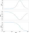 |
Fig. 1. Quantities corresponding to the fiducial case. The top plot is the magnetization, and the middle and bottom plots are the toroidal and poloidal components of the magnetic field, respectively. |
Parameters for the fiducial cases examined.
Equation (4) is used to find the value of B0 given ρ0 and the value of σ measured on the boundary of the jet. Also, we adopt the Matthews–Taub equation of state, which provides the formula for the specific enthalpy as a function of Θ = P/ρ0 (cf. Eq. (13) in Mignone & McKinney 2007).
The jet is assumed to be surrounded by a static environment. This creates a top-hat profile for the jet–environment system as the jet has a constant velocity up to the jet radius, which drops to zero for the environment. The pressure of the environment can be hydrodynamic or can only have magnetic field and zero thermal pressure (cold environment). In the case of the magnetized environment, the magnetic field is along the z-direction. We also assume a constant value for both the density and the pressure or the magnetic field profile. The environment is in pressure balance with the jet.
3. Linear stability analysis
3.1. Linearization
In order to study the stability properties of the outflows in the linear regime, we need to perturb the RMHD set of equations. This can be achieved by inserting small perturbations for every physical quantity, Q(ϖ, ϕ, z, t) = Q0(ϖ)+δQ(ϖ, ϕ, z, t), and we linearize the equations with respect to the perturbations. The zeroth-order quantities depend only on the radius, and so we can analyze the perturbations into Fourier parts, δQ(ϖ, ϕ, z, t) = Q1(ϖ)exp[i(−ωt + kz + mϕ)].
As for the Fourier transform variables, k is a real number and m is an integer, while ω = Re(ω) + iIm(ω) is a complex number, because we adopt the temporal approach. Essentially, the amplitude of the instabilities is time dependent, and modes with Im(ω) > 0 are deemed unstable, while modes with Im(ω) ≤ 0 are characterized as stable. This can be seen by inserting ω into the perturbation formula, which takes the form δQ = Q1exp[Im(ω)t]exp[i(−Re(ω)t+kz+mϕ)], where the time-dependent amplitude is the product Q1exp[Im(ω)t].
After applying the proper algebra, the final linearized system can be written as (V23):
 (5)
(5)
where  is associated to the Lagrangian displacement,
  is the total pressure perturbation and ω0 = ω − kVz − mVϕ/ϖ. These two variables are the unknowns of our system, while the ℱ and 𝒟 coefficients are complicated expressions of the unperturbed quantities, their respective derivatives, and also factors related to the Fourier transform (k, m, ω).
3.2. Boundary conditions
Regarding the boundary conditions, there are three points of interest in our computational box. The first is the axis of the jet (ϖ = 0), where we require the solutions to remain finite. For very long distances from the jet (ϖ → ∞), the solutions need to vanish.
The final point of interest is the boundary surface of the jet where y1 and y2 are required to be continuous. This statement is equivalent to
 (6)
(6)
 (7)
(7)
3.3. Solutions
The computational domain consists of two distinct areas. The first is the jet ϖ ≤ ϖj and the second is the surrounding medium ϖ > ϖj. As mentioned in Sect. 2, the environment is considered static, with a constant profile for the density. The pressure can be either purely thermal or purely magnetic and is also assumed constant. In the case of a magnetized environment, the magnetic field has only a z-component. Under these assumptions, the system of Eq. (5) yields a Bessel differential equation, the solution of which is a Hankel function of the first kind (see, e.g., Hardee 2007),  (for the full analysis of the solution derivation and the argument of the Hankel function, we refer to Sect. 5.1 of V23).
The choice of  is based on the asymptotic behavior of the function for ϖ ≫ ϖj, as it represents a wave propagating away from the jet with diminishing amplitude. Importantly, we require that there be no perturbations originating from large distances away from the jet, which are able to affect the configuration.
The system of Eq. (5) for the interior of the jet is perplexed, making it very difficult to find analytic solutions. Almost every configuration is treated numerically, and so we utilize a shooting method in order to find the unstable modes. The integration starts from a point in the proximity of the axis and ends on the boundary of the jet, where the boundary conditions (6) and (7) are applied. For details of the expressions, their derivation, and the boundary conditions on the rotation axis, we refer to V23.
4. Results
4.1. Parametric study of Kelvin–Helmholtz mode Fiducial case
While probing the stability properties of case F, we came across a specific mode on which we focus our analysis. The dispersion relation of the configuration for m = 0 can be viewed in Fig. 2, where we remind the reader that the units for ω and k are c/ϖj and 1/ϖj, respectively. Solid and dashed lines represent the real and imaginary part of ω, respectively, and the specific solution mentioned earlier is shown in red. The dashed line values are Im(ω) ≳ 1 for k ≳ 10 meaning that the instability growth timescales are comparable to the light crossing time of the jet radius. Additionally, the analysis in the present section reveals a number of traits for this specific solution, such as the locality of the mode and the linear dependence of Im(ω) on k, among others. These traits link to an established and well-studied instability in the literature, the Kelvin–Helmholtz instability. Here, we analyze a generalized relativistic equivalent in a cylindrical configuration. For brevity, the Kelvin-Helmholtz mode is denoted KH from this point onwards.
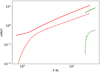 |
Fig. 2. Dispersion relation plot for the KH mode (solution show in red). The solid line represents Re(ω) while the dashed line shows Im(ω). This dispersion plot corresponds to case F and the environment is hydrodynamic. |
The mode shows a linear relation of Im(ω) with k (Im(ω) ∝ k) for k ≳ 2. This proportionality does not hold as k decreases, and so the linearity stops at k ∼ 2 and the mode becomes stable through a cut-off at k ∼ 1. It should be noted that every other mode has Im(ω) values, which are much smaller than in the KH solution, such as the green-colored mode in Fig. 2. The mode starts at k ∼ 20 and the Im(ω) ∼ 0.3 for k ∼ 30. At this wavenumber, the dashed colored line has a value of ∼4, and therefore the KH mode is much more unstable than the green-colored mode. Also, there are other possible solutions for even higher wavenumbers, but their respective Im(ω) are not comparable with the equivalent of the KH mode. KH instability will surely be the first to emanate and disrupt the initial configuration, outpacing every other mode.
In Fig. 3 we plot the dispersion relation of the KH mode when the environment of the jet is magnetized. The dispersion relation is quite similar to the respective one in Fig. 2. The imaginary part is proportional to the wavenumber for k ≳ 2 and Im(ω) ≳ 1 for k ≳ 10. The linearity stops for k ∼ 2 and the mode stabilizes via a cut-off at k ≃ 1. The next solution is found for k ≫ 20 and has Im(ω) ≪ Im(ω)KH, and so we do not include it in Fig. 3. In both Figs. 2 and 3, other solutions apart from the KH mode are sparse. The instability profile of the jet is KH mode dominated.
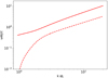 |
Fig. 3. Dispersion relation plot for the KH mode (solution show in red) for case F when the environment of the jet is magnetized. The solid line represents Re(ω) while the dashed line shows Im(ω). |
Apart from m = 0, the KH mode was also found for m ≠ 0. We opted to check four other cases with m = ±1, ± 3. In Fig. 4, we plot  for the KH mode versus the corresponding m, while k = π. For m ± 3, the mode attains smaller Im(ω) values than in all other cases. For m = −3, Im(ω) ≈ 0.05 and for m = 3, Im(ω) ≈ 0.14. Then for m = 0, ± 1, the Im(ω) values are very close and approximately equal to 0.21. We note that m = 0 is, by a small margin, the most unstable, followed by m = 1 and m = −1, respectively. As m increases, the Im(ω) decreases; the mechanism for this behavior is discussed in Sect. 5.
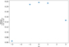 |
Fig. 4.
|

This linearity of Im(ω) gives us the chance to study the mode without having to plot the solution for multiple wavenumbers. The results are easily generalized simply by calculating the difference in the value of Im(ω) in relation to the change in k, and so we focus our analysis on this component.
In this section, we present a parametric stability analysis. We start by probing our fiducial configuration, which is denoted case “F” and the configuration is described in Sect. 2. The density profile is constant and the parameter values are shown in Table 1. Parameter η is the ratio of the rest mass density of the environment to that of the jet, η = ρe/ρ0.
This study focuses on the axisymmetric mode, as it is the most unstable. For the parametric study that follows, the wavenumber is fixed to k = π, corresponding to the wavelength equal to the jet diameter.
4.1.1. Dependence of the KH mode on the density ratio (η)
The first parameter under consideration is the density rest mass ratio, η. We discuss both purely thermal and magnetized environments depicted in Figs. 5 and 6, respectively. The parameter spans a wide value range from sparse environments (η = 10−2) to very dense counterparts (η = 102 − 103).
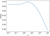 |
Fig. 5. Im(ω) versus density ratio η for case F and a jet in a hydrodynamic environment. |
Figure 5 shows Im(ω) versus η for the thermal environment. For η ≤ 1, a plateau of constant Im(ω) ≃ 0.7 is formed, while from η ≃ 1 up to η ≃ 10, a small increase in the value is noted. For higher ratio values, the Im(ω) decreases, and for η ∼ 103, Im(ω) has dropped down to ∼0.4. Therefore, the increase in the density of the environment generally stabilizes the mode, while for a wide range of the parameter value (η ≤ 1), the mode seems to not be affected by any change in η.
Figure 6 shows Im(ω) versus η in the case of a jet with a magnetized environment. Initially, we note a cutoff at η ∼ 1, and then the Im(ω) increases monotonically up until its maximum value of Im(ω) ≃ 0.6 for η ∼ 30. After this maximum, a decrease starts towards higher η. The maximum Im(ω) for the magnetized environment is smaller than for the thermal equivalent.
Figures 5 and 6 suggest different mode behavior regarding the pressure-providing mechanism of the environment, with the magnetized environment being more stable than its thermal counterpart. When we have magnetized environment, the KH mode is stabilized for η ≲ 1. The thermal environment solution spans a greater range of η and has higher maximum Im(ω). Clearly, the two different kinds of environment lead to different results, meaning that the physics of the medium supporting the jet is an important factor. In general, denser environments stabilize the mode either by entirely eliminating Im(ω) or sufficiently reducing it.
4.1.2. Dependence of the KH mode on the magnetization (σ)
Moving on, we study how the magnetization of the jet affects the growth rate. We note that the magnetization value is calculated for ϖ = ϖj along every other quantity that is radius dependent. The reason for making this choice is extensively discussed in Sects. 4.4 and 4.3. At this point, it suffices to state that we have observed that only the conditions of the region around the jet boundary are important for the KH mode. We begin with Fig. 7, for which the environment is hydrodynamic. Clearly, the increase in the magnetization leads to an increase in Im(ω). For σ ≪ 1 and σ ≫ 1, the Im(ω) becomes approximately constant. For σ ≪ 1, Im(ω) → 0, while for Im(ω) ≫ 1, Im(ω) ≃ 0.8. The transition between these two extremes occurs at σ ∼ 1.
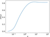 |
Fig. 7. Im(ω) versus magnetization σ for case F and a jet in a hydrodynamic environment. |
Figure 8 presents Im(ω) versus σ for a magnetized environment. When σ ≪ 1, Im(ω) → 0, similarly to Fig. 7. As magnetization increases, the imaginary part of ω also increases and reaches its maximum, Im(ω) ≃ 0.5, at σ ≃ 1. Immediately after this maximum, a steep descent follows and the instability effectively vanishes at σ ≃ 4. Importantly, the KH mode is active only for a specific range of σ, contrary to the hydrodynamic counterpart for which this range is much more extended towards the higher σ values.
Also, the maximum Im(ω) between the two cases is different, as the thermodynamic environment shows higher Im(ω) values compared to the magnetized equivalent. In general, the magnetized environment seems to weaken the instability strength and even stabilize the mode entirely for the highly magnetized jets.
4.1.3. Dependence of KH mode on the Lorentz factor (σ)
In this section, we explore the relation between Im(ω) and the Lorentz factor. In Figs. 9 and 10, we present the plots of Im(ω) versus γ for thermal and magnetized environment, respectively. Specifically, instead of γ, we plot the Im(ω) versus the proper jet velocity,  .
.
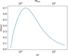 |
Fig. 9. Im(ω) versus the proper velocity of the outflow γυ for case F. The environment of the jet is hydrodynamic. The plot incorporates a secondary axis on the top edge of the plot box. The axis shows the proper fast magnetosonic Mach number. |
Starting with the hydrodynamic environment (Fig. 9), we first note that the KH mode is active for a specific velocity range. The mode disappears for γυ ≲ 0.5 and its maximum is located near this cut-off with Im(ω) ∼ 0.7 for γυ ∼ 1. After the maximum, the Im(ω) decreases with increasing γ, attaining a value of Im(ω) ∼ 0.2 for γυ ≃ 10. This means that the effective range for the instability is set between γυ ≳ 0.5 and roughly γυ ≲ 10 − 15. The axis at the top of the plot shows the proper fast magnetosonic Mach number. The relation providing this Mach number is given by Mfast = γυ/(γfυf), where  . It can be seen that for a cold jet,
  (cf. Appendix C of Vlahakis & Königl 2003). For the fiducial setup, γfυf = 1, and therefore the two horizontal axes are identical. We see that the instability is in a hinderance for ultrafast magnetosonic velocities, with its maximum being close to Mfast ∼ 1. In general, the KH mode is significantly less unstable for both ultrarelativistic and nonrelativistic configurations.
In Fig. 10 the configuration with the magnetized environment is shown. Once more, the mode lies in a specific range regarding the γ value. Similar to Fig. 9 for γυ ≃ 10 the Im(ω) ≃ 0.2. The maximum is located at γυ ∼ 2 and has a value of Im(ω) ∼ 0.5. As the flow velocity further decreases, a cut–off is formed, where the mode stabilizes at γυ ≃ 1. Hence, jets with γυ ≲ 1 ⇒ γ ≲ 1.4 are not affected by the KH mode when the environment is magnetized. The mode becomes most unstable for Mfast ≈ 2 and vanishes for ultrafast magnetosonic velocities.
The magnetized environment negatively affects the KH mode, which is similar to the situations described in Sects. 4.1.1 and 4.1.2; it decreases both the value of the maximum Im(ω) and the γ range for which the jet is being affected by the mode.
4.1.4. Dependence of the KH mode on the ratio of the magnetic field components (ϖ0)
The next parameter to take into consideration is ϖ0. As can be seen in Eq. (8), ϖ0 is directly associated with the ratio of the magnetic field components in the co-moving reference frame,
 (8)
(8)
In the central source frame, the ratio is equal to ϖ0/(ϖγ). Changing the value of ϖ0 affects which component of the jet is dominant over the other. In order to better understand the effect ϖ0 has on Bz/|Bϕ, co|, we keep the z-component of the magnetic field constant and vary only the toroidal counterpart, thereby isolating the effect Bϕ has on the KH mode. This is done by fixing the value of Bz|ϖ ≃ ϖj to that corresponding to the fiducial case F. The variation in ϖ0 then only changes the value of the toroidal magnetic field.
Figure 11 presents the Im(ω) versus ϖ0 for the hydrodynamic environment. For ϖ0 ≪ 1, the Im(ω) has an approximately constant value ≈0.8. As ϖ0 increases, the Im(ω) decreases, especially after ϖ0 ≈ 0.1. At this particular value, a cut-off is formed, leading to the subsequent mode stabilization (Im(ω) → 0).
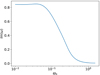 |
Fig. 11. Im(ω) versus the ratio between magnetic field components ϖ0 for case F. The jet is in a hydrodynamic environment. |
In Fig. 12, the environment is magnetized. The two plots are quite different. For ϖ0 ≈ 0.05, we note the inhibition of the mode through a cut-off. The growth rate becomes maximum for ϖ0 ≈ 0.1 with Im(ω) ≈ 0.5 and then decreases as ϖ0 further increases. For both Figs. 11 and 12, the instability has already been stabilized when ϖ0 becomes equal to 1. The hydrodynamic environment case has larger maximum Im(ω) compared to the magnetized counterpart. In summary, for both scenarios, it seems that when Bz/|Bϕ, co| ≥ 1 the KH mode is stabilized.
4.2. Alternative configuration, γ = 5
In this section, we discuss an alternate configuration to case F. The setup is identical to the previous case, apart from the Lorentz factor, which is set to γ = 5. We denote the new configuration as F5 and the fiducial values of its parameters are also summarized in Table 1, including the corresponding ω when k = π. In Fig. 13, we present the dispersion relation for this modified setup. The KH is denoted by the red lines. The Im(ω) clearly increases with k, but does not show a strict linear dependence on it. There are also numerous solutions whose Im(ω) become comparable to the KH Im(ω) value as k increases. Some of them are ∝k (yellow- and brown-colored solutions) but as the blue-colored mode ceases to be linear for sufficiently large k, it is possible that the rest of the modes behave similarly.
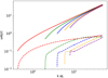 |
Fig. 13. Dispersion relation plot for KH mode (red colored solution) for the alternative configuration (case F5), for which the Lorentz factor γ = 5. |
It should be noted that the physical mechanism of these new modes could be different from that of the KH solution. This was probed via a multiple η test, where we increased the density ratio to η = 100. This resulted in the elimination of the KH mode but did not affect any of the other modes at all. This trait is typical of current-driven instabilities (Appl et al. 2000) and these solutions could be linked to this type of instability. These modes will be studied in a future work.
Following the structure of Sect. 4.1, we present our parametric study of the stability analysis for the F5 configuration, regarding η, σ, and ϖ0 for both hydrodynamic and magnetized environment.
4.2.1. Alternative configuration: Dependence of the KH mode on density ratio (η)
Beginning with the density ratio, Figs. 14 and 15 show the Im(ω) versus η for hydrodynamic and magnetized environment, respectively. Both plots resemble Figs. 5 and 6, except for a few details. In general, we observe smaller Im(ω) values across the whole η range. This could already be expected given the result of Im(ω) versus γ in Sect. 4.1.3, where for γ = 5 ⇒ γυ ≃ 5 the Im(ω) is substantially smaller than the corresponding value for γ ∼ 2.
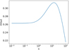 |
Fig. 14. Im(ω) versus density ratio η for the alternative configuration F5. The environment is hydrodynamic. |
In Fig. 14 we once more observe a plateau of constant value for η ≪ 1. As η increases, the Im(ω) also increases starting from η ≈ 1 up to η ≈ 20, where its maximum is reached. The amount of total increase in Im(ω) is quite substantial, whereas this trend in case F is almost negligible. Then, as η further increases, the mode begins to weaken and shows a stabilizing behavior for η ≫ 1.
In a magnetized environment (Fig. 15), the behavior of Im(ω) appears almost identical to that seen in Fig. 6. Apart from the smaller Im(ω) values, the distribution in Fig. 15 has its maximum slightly shifted towards smaller η. The mode is stabilized at η ≈ 0.2, which is just a little less than the respective value in case F.
4.2.2. Alternative configuration: Dependence of the KH mode on magnetization (σ)
As in Sect. 4.1.2, we probe the dependence of the KH mode on the value of the magnetization for ϖ ≈ ϖj. In Fig. 16, we plot the Im(ω) versus σ for the hydrodynamic environment. Figures 7 and 16 are similar, presenting two constant values of Im(ω) for σ ≪ 1 and σ ≫ 1, respectively. The instability is favored by highly magnetized configurations, while as σ decreases the mode fades out. The transition between the two plateaus, similarly to Fig. 7, occurs at σ ∼ 1.
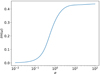 |
Fig. 16. Im(ω) versus magnetization σ for the alternative configuration F5. The environment is hydrodynamic. |
Figure 17 presents results corresponding to the magnetized environment. The mode is stabilized for both σ ≪ 1 and σ ≳ 20. The decrease for σ ≳ 3 is quite steep. The maximum is located at σ ≈ 3, which is slightly higher than the corresponding value in Fig. 8. The Im(ω) values, in general, are smaller compared to the ones in Fig. 8. Overall, the results regarding magnetization are in line with the results of Sect. 4.1.2.
4.2.3. Alternative configuration: Dependence of the KH mode on the ratio of the magnetic field components (ϖ0)
Finally, we present the results for Im(ω) versus ϖ0 for both hydrodynamic and magnetized environment. Figure 18 depicts results for the hydrodynamic environment. As in Fig. 11, the mode is favored by small ϖ0, specifically ϖ0 ≲ 0.1. While ϖ0 decreases further below 0.1, the mode shows a slight increase in Im(ω). This trait is not present in Fig. 11. For ϖ0 ≳ 0.1, the Im(ω) decreases rapidly until ϖ0 ≈ 1, where the Im(ω) becomes negligible.
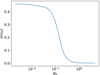 |
Fig. 18. Im(ω) versus the ratio of the magnetic field components ϖ0 for the alternative configuration F5. The environment is hydrodynamic. |
Figure 19 shows Im(ω) versus ϖ0 for the magnetized environment. Similar to the hydrodynamic counterpart, Figs. 19 and 12 present substantial similarities. The mode is stabilized for ϖ0 ≪ 1 and ϖ0 ≫ 1, while the maximum is located at ϖ0 ≈ 0.1, with Im(ω) ≈ 0.35. The maximum Im(ω) is smaller than the corresponding value for case F. The mode is effectively stabilized for ϖ0 ≈ 10−2 through a steep descent.
4.3. Eigenfunctions
The eigenfunctions for the fiducial case (case F) are depicted in Fig. 20. The top panel shows y1 and in the bottom panel shows y2 for k = π. We show both the real and the imaginary component for each eigenfunction. Beginning with y1, we observe that both the real and the imaginary part have their respective maxima in the vicinity of the jet boundary surface. This indicates that the jet’s flow lines are going to be displaced mainly in the area where ϖ ≈ ϖj. Lagrangian displacement diminishes for both ϖ → 0 and ϖ → ∞.
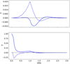 |
Fig. 20. Eigenfunctions in case F. The top plot shows y1 and the bottom plot shows y2. Solid and dashed lines represent the real and the imaginary part of the eigenfunctions. |
For y2, we observe different traits compared to y1. Both components tend to present their global maxima near the axis of the jet. As radius increases, the eigenfunction’s components decrease in value, but upon closer inspection we see that both real and imaginary parts present local maxima in the vicinity of the boundary. This means that both eigenfunctions share the trend of localized activity at ϖ ≈ ϖj. The heightened values of y2 for ϖ → 0 could be due to the reflection of waves on the axis of the jet. Therefore, the main scenario is that the mode is mostly local; it is created on the boundary of the jet and propagates towards the axis and the ambient medium.
In order to provide clearer evidence for the previous statement, in Fig. 21 we plot the eigenfunctions for the fiducial case, and for k = 10. Evidently, both eigenfunctions are well established in the neighborhood of the jet boundary; they diminish rapidly propagating away from this surface, and therefore the maximum intensity of the mode is expected to be at ϖ ≈ ϖj.
Figure 22 presents the eigenfunctions for case F5. Both y1 and y2 present their maxima near the boundary of the jet. The total pressure perturbation shows evidence of possible reflection similar to that seen in Fig. 20. One important difference is that the mode does not decrease rapidly as the radius changes from ϖj. Particularly for Im(y2), the mode gradually decreases towards the axis of the jet, while both eigenfunctions decrease smoothly as ϖ → ∞. This result alongside the variation from the strict linear behavior in Fig. 13 could suggest that, as γ changes, the solution progressively transforms to a different kind of instability that is similar but not identical to the KH mode.
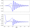 |
Fig. 22. Eigenfunctions for alternative configuration F5. The top and bottom plots correspond to y1 and y2, respectively. Solid and dashed lines represent the real and the imaginary part of the eigenfunctions. |
4.4. WKBJ approximation
Our analysis of the KH mode eigenfunctions in Sect. 4.3 supports the idea that the solution is localized, that is, the mode emanates and affects mainly a specific portion of the cross-section of the jet and not the entirety of the configuration. To further test this claim, we apply the WKBJ approximation to zeroth order to the fiducial configuration, case F. A thorough description of the WKBJ approximation on the linearized RMHD set of equations can be found in Sect. 4 of V23. We apply the WKBJ methodology to the system of Eq. (5) at the jet radius, ϖ ≈ ϖj. We only present and discuss results for the hydrodynamic environment, but we confirm that similar conclusions also apply to the magnetized counterpart. Figures 23–26 show Im(ω) versus η, σ, γ, and ϖ0, respectively.
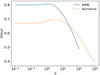 |
Fig. 23. Im(ω) versus density ratio η for the fiducial case F with a hydrodynamic environment. This plot compares results from the WKBJ approximation and the full numerical methodology. The WKBJ solution is depicted with blue solid lines and the numerical results are depicted with the orange dashed lines. |
The main result is that the WKBJ predictions are in good agreement with the full numerical counterpart. The best fit can be seen in Fig. 25, which depicts the Im(ω) versus γ. Over the whole γ range, the solid and dashed lines are close, especially for γ ≳ 3.
Regarding σ and ϖ0, we also observe good agreement between the two methods. The overall behavior of the solutions is predicted correctly by the WKBJ approximation. It is really important that the transitions in both plots between the stabilized and nonstabilized states is found to occur at the same parameter values. The least successful comparison between WKBJ and the full numerical treatise is noted for the density ratio in Fig. 23. The WKBJ methodology overestimates Im(ω) for the majority of the range of η; nonetheless, the general behavior of Im(ω) versus η is predicted correctly and the error is not more than ∼20%.
It should be highlighted that the WKBJ prediction accuracy relies heavily on the value of k. As k increases, the results from the two methods tend to be even closer. Figure 27 is similar to Fig. 23, but for k = 10. The convergence between the two solutions is relatively good, and most importantly is much better than the corresponding convergence seen for k = π. The solid line is able to follow the dashed counterpart more closely.
4.5. Comparison with Kelvin–Helmholtz instability in Cartesian geometry
Relativistic Kelvin–Helmholtz has already been studied assuming Cartesian geometry for a variety of configurations (e.g., Bodo et al. 1994; Osmanov et al. 2008; Chow et al. 2023a,b). Results from Sect. 4.1 suggest a possible relation between the Kelvin-Helmholtz from the cylindrical jet and the Cartesian counterpart. As an example, the linear relation of Im(ω) with k is an indicative element, as in the Cartesian geometry the Kelvin-Helmholtz instability is characterized by Im(ω) ∝ k across the entire range of k values. It is therefore interesting to compare the results for the cylindrical jet with the KH results generated for a planar geometry.
To this end, we assume two planar flows in contact along the yz surface. The first is the “jet”, which has relativistic velocity along the z-direction, while the second is static and we consider it to be the “environment”. Essentially, we replicate the configuration of Sect. 2 in Cartesian geometry. Therefore, for the jet, we have γ = 2, ρ0 = 1, and P = 0, and for the magnetic field we adopt Eqs. (2) and (3) at ϖ = ϖj, that is, Bz|cartesian = Bz(ϖj) and By|cartesian = Bϕ(ϖj). The environment is assumed to be nonmagnetized, with constant pressure and density profiles. Below we present parametric plots of Im(ω) versus η, σ, and γ for different values of k.
We are able to obtain the Cartesian dispersion relation by approximating the cylindrical system for ϖ ⋙ 1. The cylindrical wavenumber components can be related to the Cartesian counterparts as m/ϖ → ky, k → kz. V23 discuss when the equations give the corresponding ones for the planar geometry, and the radial wavenumber is given by  (Eq. (53) in V23). The ℱ symbols are provided by Eqs. (54)–(57) in V23, with the second term in ℱ21/𝒟 omitted. The dispersion relation can be written in the following form:
 (9)
(9)
where  (including the radial part), kcoz = γ(kz−ωV), and
  , and
, and  is the proper Alfvén velocity. The quantities of the environment are denoted with the subscript “e”.
Figure 28 shows Im(ω)/k versus σ for case F and for k = π, 10. The solid line represents the Cartesian solution while orange and green dashed lines represent the results from the cylindrical system for k = π, 10, respectively. The solid line indicates stabilization for the mode at σ ≈ 0.5. As σ increases, the value of Im(ω) also increases. For σ ≳ 10, the rate of increase for Im(ω) becomes smaller, and the Im(ω) values form a plateau-like region. The solid line overestimates and underestimates the Im(ω) values for σ > 2, σ < 2 respectively. For σ ≲ 0.5, both of the cylindrical results are not immediately stabilized as they are in the Cartesian solution. When we set k = 10, we notice that the blue line is much closer to the cylindrical counterpart, as the differences in Im(ω) values of the two lines are much smaller. Briefly, as k increases the solid line tends to approximate the dashed lines quite successfully.
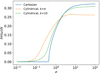 |
Fig. 28. Im(ω)/k versus σ for case F. The jet is surrounded by a hydrodynamic environment. The solid line represents the solution in Cartesian geometry and the dashed lines show the solution in cylindrical geometry for k = π, 10. |
Figure 29 shows Im(ω)/k versus η for case F. Similarly to Fig. 28, the solid line is the result corresponding to the Cartesian geometry and the dashed lines correspond to the cylindrical jet for k = π, 10. We observe that the Cartesian mode has two cut-offs with values γυ ∼ 0.1 and γυ ∼ 4, respectively. The cylindrical solutions present a cut-off at γυ ∼ 0.2 − 0.5 while they diminish gradually for increasing Lorentz factor values beyond γυ ∼ 1. As k becomes larger, the blue solid line starts to converge with the cylindrical solution, as also observed in Fig. 28. For larger γυ values, the stabilization of the cylindrical mode becomes less gradual, while the lower cut-off is closer to the Cartesian counterpart.
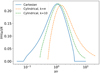 |
Fig. 29. Im(ω)/k versus σ for case F. The jet is surrounded by a hydrodynamic environment. The solid line represents the solution in a Cartesian geometry and the dashed line represents that in a cylindrical geometry for k = π, 10. |
Similar to Figs. 28 and 29, we plot Im(ω)/k versus η in Fig. 30. This plot includes an extra wavelength value, k = 15, depicted with the red dashed line. The Cartesian solution forms a plateau for Im(ω) values when η ≲ 1. For η ≳ 1, the Im(ω) values decrease up until η ∼ 20, where the KH mode fully stabilizes. The cylindrical solutions also form a plateau for η ≲ 1 similar to the planar geometry. For η ≳ 1, the Im(ω) decreases but does not fully stabilize for η ∼ 20. Once more, we observe that, as k increases, the Cartesian solution begins to approximate the cylindrical equivalent more precisely. In this plot, we include the extra wavelength (k = 15) to emphasize the fact that increasing k values further aids the Cartesian solution to follow the behavior of the cylindrical mode.
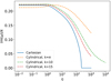 |
Fig. 30. Im(ω)/k versus η for case F. The jet is surrounded by a hydrodynamic environment. The solid line represents the solution in a Cartesian geometry and the dashed line shows that in a cylindrical geometry for k = π, 10, 15. |
It is evident that the Cartesian geometry successfully predicts the KH mode of the cylindrical geometry, and the quality of the prediction is enhanced as k increases. More specifically, there are three length scales involved into the efficient approximation of the cylindrical geometry by the Cartesian counterpart. The first is the wavenumber k, the second is the  and the last one is the wavelength of the Hankel function’s argument λ; these are defined and analyzed in Sects. 5 and 5.1 of V23. Our analysis indicates that the cylindrical geometry can be omitted whenever k ≫ 1/ϖj,
  , and λ ≫ 1/ϖj. Hence, there are three length scale relations that need to be fulfilled simultaneously. Each of them needs to be much larger than the radius of the jet so that the curvature of the cylindrical jet can be discarded and the planar approximation is valid.
5. Discussion and conclusions
In this study, we conducted a linear stability analysis of a cylindrical relativistic magnetized jet. The unperturbed outflow is in force balance with its environment, includes a helical magnetic field, and does not have thermal pressure. We chose to study axisymmetric solutions as they are found to be the most unstable. During the analysis, a rapidly growing mode arose that showed instabilities with growth timescales comparable to the light crossing time of the jet radius. Also, the solutions present a linear relation between Im(ω) and k (Im(ω) ∝ k), which is typical of the Kelvin-Helmholtz mode in Cartesian geometry. As wavenumber decreases, the solution vanishes via a cut-off at k ∼ 1, and so the cylindrical counterpart does not extend to k → 0. This is not the case for the Cartesian KH for which as k → 0 ⇒ Im(ω) → 0.
In order to fully understand the relation between this mode and the various outflow parameters, we proceeded with a parametric study regarding the ratio of the rest mass density of the jet to that of the environment (η), the jet’s Lorentz factor (γ), the magnetization (σ), and the ratio of the magnetic field’s poloidal component to the toroidal component measured in the co-moving frame of reference (ϖ0). Also, we tested whether the mode is affected by the pressure-providing mechanism of the environment (thermal or magnetic pressure).
The mode is favored by jets that are denser than their environment. Im(ω) diminishes with increasing η, while it retains a constant high value for η ≪ 1. When the environment becomes magnetized, the plateau for Im(ω) disappears and the mode is stabilized for η ≲ 1. For η ≫ 1, the increased inertia of the environment is a prominent factor for the stabilization of the KH mode.
Next, we examined the effect of Im(ω) on the magnetization value. In general, increasing σ leads to more unstable configurations. The instability weakens when the configuration becomes less magnetized. The change on σ was made by properly altering the amplitude of the magnetic field B0. When the environment becomes magnetized, the mode terminates via a cut-off at σ ≈ 4. The main element affecting this result is the presence of the magnetic field in the environment. As σ increases, so does the external magnetic field in order to provide adequate pressure to support the jet. When the instability emanates and starts displacing the field lines, the tension from the external magnetic field will be more intense for large σ values. Finally, for even higher σ, the jet cannot overcome the tension and the KH mode is stabilized.
We continued our analysis with the dependence of Im(ω) on the Lorentz factor value. This parameter also affects the KH mode, as the solution is stabilized for nonrelativistic velocities. This also happens for Lorentz factors γ ≳ 8, as the Im(ω) gradually decreases with increasing Lorentz factor value for γ ≳ 2. The maximum growth for the KH mode is observed for γ ≃ 2. When the environment becomes magnetized, the general behavior remains similar except for the small γ. The cut-off changes from γ ∼ 1 to γ ≈ 1.4, stabilizing a group of mildly relativistic configurations. In general, the magnetized environment hinders the mode. A similar result is seen in Fig. 9 of Bodo et al. (2013), which is quite similar to both Figs. 9 and 10.
In Figs. 11 and 12, we analyze the relation of Im(ω) versus ϖ0. The physical quantity related to ϖ0 is the ratio of the magnetic field components measured on the boundary of the jet in the co-moving frame, Bz/|Bϕ, co|. The most important result is the rapid stabilization of the mode when Bz/|Bϕ, co| ∼ 1. The poloidal component of the magnetic field fully suppresses the mode. Technically, we opted to fix the value of Bz and change Bϕ. We are therefore also able to state that, when Bϕ becomes negligible compared to Bz, the mode is weakened. The toroidal component of the magnetic field seems to be an integral element of the mechanism that generates the KH solution.
At this point, it is important to note that our results can also be characterized by the angle of the magnetic field with the wavevector k. In our case, the wavevector is always parallel to the z-direction, and therefore we essentially measure cos(θ) = Bz/||Bco||, where  . This angle can be related to the ϖ0 parameter through
  . For case F, the angle between Bco and k is ≃π/2.
In order to better understand the dependence on ϖ0, one should note that by changing ϖ0 we also change the angle between the magnetic field and the z-direction (or equivalently the k). When ϖ0 ≫ 1 ⇒ cos(θ)→1, which means that the magnetic field tends to align with the wavevector. In this scenario, the instability needs to overcome the increased tension provided by the aligned magnetic field and leading to the inhibition of the KH mode. On the contrary, when Bco ⊥ k, the effect of the magnetic field’s tension on the instability is minimized.
The magnetic tension effect also explains why the axisymmetric mode is the most unstable, as seen in Fig. 4. As |m| increases, the angle between the co-moving magnetic field and the wavenumber decreases, and therefore the instability needs to overcome the increased tension of the magnetic field. This leads to the instability inhibition and to lower growth rates.
The eigenfunctions of the mode present an exponential increase near the boundary of the jet. This trait is found in both the jet and the environment near their common interface. The mode fades out for ϖ → 0 and ϖ → ∞. The rate of descent for both directions is relatively intense, implying that the rest of the jet remains unaffected. This result establishes the notion of the locality for the KH mode. The spatial range of the instability’s effect on the configuration is local and exhibited mainly near the boundary surface of the jet. Also, the KH mode profile is shaped by the local jet configuration at ϖ ≈ ϖj, while the rest of the jet and environment are disregarded.
In order to test the locality of the KH mode, we applied a WKBJ approximation on the system of Eq. (5) for ϖ = ϖj. We noticed that the WKBJ serves as an efficient proxy for the ω values of the mode. This behavior is enhanced when k is increased. It is imperative to highlight the fact that the WKBJ approximation does not take into consideration the behavior of the solution near the jet’s axis, nor towards infinity. This means that the provided efficiency of the WKBJ method reinforces the conclusions provided by the analysis of the eigenfunctions.
Next, we considered an alternative configuration, which has γ = 5, compared to the fiducial case, which has γ = 2. The results of Sect. 4.2 only consider a hydrodynamic environment surrounding the jet. In general, the parametric study reveals that the KH mode in the alternative configuration is related to the corresponding mode for the fiducial setup but is not identical. It is evident that there are differences between the two cases. First of all, in Fig. 13 the mode is not linear with respect to k and the ω-plane is full of other modes that are not present in the fiducial setup with γ = 2. In Fig. 22, the eigenfunctions are not concentrated around ϖ ≈ ϖj. Here, y1 and y2 extend with nonzero values for ϖ < ϖj, while for ϖ > ϖj, the eigenfunctions diminish gradually as ϖ increases. On the other hand, the WKBJ correctly predicts the growth rate of the instability. Moreover, the parametric study suggests that the behavior of the KH mode of the alternative configuration is similar to the corresponding behavior of the fiducial case, besides the fact that the growth rates are in general lower.
These results could indicate that the KH mode fuses with other types of instability, such as the current-driven modes. This way, the instability retains its traits even if they are mildly modified compared to the results for the fiducial case. This phenomenon is also noted in Bodo et al. (2013), where the KH and current-driven instabilities cannot be distinguished for a relativistic jet with a helical magnetic field.
Finally, we made the comparison between the KH mode in cylindrical and Cartesian geometry, respectively. This was based on the existence of various common traits of the KH mode in both geometries, which are Im(ω) ∝ k, the locality of the mode, the effect that the angle between Bco and k has on the instability, and finally the decrease in Im(ω) while Mfast increases. Our analysis allowed us to establish a definite criterion regarding the characteristic length scales of the system. This criterion requires that  simultaneously. Whenever this is fulfilled, the cylindrical geometry can be discarded and the results can be approximated by the Cartesian KH instability.
Various traits of the KH mode can be identified in publications studying the Cartesian KH instability. For example the dependence of the mode’s intensity on the angle between Bco and k was also observed to be crucial by Osmanov et al. (2008), Chow et al. (2023a,b). The cut-off for small Mfast values is also discussed in Chow et al. (2023a), where the “jet” velocities need to be super-Alfvénic. High-density contrasts between the two fluids lead to stabilization of the KH mode Ferrari et al. (1980). Nonetheless, we show here that the cylindrical KH mode is not identical to the Cartesian counterpart and the properties of the KH instability emanating in a jet are considerably modified.
Furthermore, the KH instability could have substantial implications for the phenomenology of the astrophysical jets. This is related to the nonlinear evolution of the modes. Most notably, the KH mode creates vortices on the boundary layer of the jet and its environment. This layer is characterized by the velocity shear between the two media. The vortices distort the field lines and twist them in such a way that a variety of phenomena may arise, such as turbulence. Moreover, this alteration of the magnetic field topology may create sites where field lines of opposite polarity can become adjacent, triggering magnetic reconnection and subsequently nonthermal particle acceleration, as discussed in Sironi et al. (2021).
The nonlinear evolution of the KH instability in astrophysical environments can only be studied numerically through MHD simulations, as in for example Millas et al. (2017), Berlok & Pfrommer (2019a,b), or using particle in cell (PIC) simulations, as in Sironi et al. (2021). We leave the study of the nonlinear evolution of the modes we find to a future paper.
Acknowledgments
This research is co-financed by Greece and the European Union (European Social Fund-ESF) through the Operational Programme “Human Resources Development, Education and Lifelong Learning” in the context of the project “Strengthening Human Resources Research Potential via Doctorate Research” (MIS-5000432), implemented by the State Scholarships Foundation (IKY).
References
- Appl, S., Lery, T., & Baty, H. 2000, A&A, 355, 818 [NASA ADS] [Google Scholar]
- Begelman, M. C. 1998, ApJ, 493, 291 [NASA ADS] [CrossRef] [Google Scholar]
- Berlok, T., & Pfrommer, C. 2019a, MNRAS, 485, 908 [NASA ADS] [CrossRef] [Google Scholar]
- Berlok, T., & Pfrommer, C. 2019b, MNRAS, 489, 3368 [NASA ADS] [CrossRef] [Google Scholar]
- Blandford, R. D., & Payne, D. G. 1982, MNRAS, 199, 883 [CrossRef] [Google Scholar]
- Blandford, R. D., & Znajek, R. L. 1977, MNRAS, 179, 433 [NASA ADS] [CrossRef] [Google Scholar]
- Bodo, G., Massaglia, S., Ferrari, A., & Trussoni, E. 1994, A&A, 283, 655 [NASA ADS] [Google Scholar]
- Bodo, G., Mignone, A., & Rosner, R. 2004, Phys. Rev. E, 70, 036304 [NASA ADS] [CrossRef] [Google Scholar]
- Bodo, G., Mamatsashvili, G., Rossi, P., & Mignone, A. 2013, MNRAS, 434, 3030 [Google Scholar]
- Bodo, G., Mamatsashvili, G., Rossi, P., & Mignone, A. 2016, MNRAS, 462, 3031 [Google Scholar]
- Bodo, G., Mamatsashvili, G., Rossi, P., & Mignone, A. 2019, MNRAS, 485, 2909 [Google Scholar]
- Chow, A., Davelaar, J., Rowan, M., & Sironi, L. 2023a, ApJ, 951, L23 [NASA ADS] [CrossRef] [Google Scholar]
- Chow, A., Rowan, M. E., Sironi, L., et al. 2023b, MNRAS, 524, 90 [CrossRef] [Google Scholar]
- Curtis, H. D. 1918, Pub. Lick Obs., 13, 9 [NASA ADS] [Google Scholar]
- Das, U., & Begelman, M. C. 2019, MNRAS, 482, 2107 [NASA ADS] [CrossRef] [Google Scholar]
- Ferrari, A., Trussoni, E., & Zaninetti, L. 1978, A&A, 64, 43 [NASA ADS] [Google Scholar]
- Ferrari, A., Trussoni, E., & Zaninetti, L. 1980, MNRAS, 193, 469 [NASA ADS] [Google Scholar]
- Ferrari, A., Trussoni, E., & Zaninetti, L. 1981, MNRAS, 196, 1051 [NASA ADS] [Google Scholar]
- Hardee, P. E. 2007, ApJ, 664, 26 [Google Scholar]
- Istomin, Y. N., & Pariev, V. I. 1996, MNRAS, 281, 1 [Google Scholar]
- Kim, J., Balsara, D. S., Lyutikov, M., et al. 2015, MNRAS, 450, 982 [Google Scholar]
- Kim, J., Balsara, D. S., Lyutikov, M., & Komissarov, S. S. 2016, MNRAS, 461, 728 [Google Scholar]
- Kim, J., Balsara, D. S., Lyutikov, M., & Komissarov, S. S. 2017, MNRAS, 467, 4647 [Google Scholar]
- Kim, J., Balsara, D. S., Lyutikov, M., & Komissarov, S. S. 2018, MNRAS, 474, 3954 [Google Scholar]
- Mignone, A., & McKinney, J. C. 2007, MNRAS, 378, 1118 [Google Scholar]
- Millas, D., Keppens, R., & Meliani, Z. 2017, MNRAS, 470, 592 [NASA ADS] [CrossRef] [Google Scholar]
- Mizuno, Y., Lyubarsky, Y., Nishikawa, K.-I., & Hardee, P. E. 2012, ApJ, 757, 16 [Google Scholar]
- Narayan, R., Li, J., & Tchekhovskoy, A. 2009, ApJ, 697, 1681 [NASA ADS] [CrossRef] [Google Scholar]
- Osmanov, Z., Mignone, A., Massaglia, S., Bodo, G., & Ferrari, A. 2008, A&A, 490, 493 [NASA ADS] [CrossRef] [EDP Sciences] [Google Scholar]
- Sironi, L., Rowan, M. E., & Narayan, R. 2021, ApJ, 907, L44 [CrossRef] [Google Scholar]
- Sobacchi, E., & Lyubarsky, Y. E. 2018, MNRAS, 473, 2813 [NASA ADS] [CrossRef] [Google Scholar]
- Sobacchi, E., Lyubarsky, Y. E., & Sormani, M. C. 2017, MNRAS, 468, 4635 [CrossRef] [Google Scholar]
- Vlahakis, N. 2004, ApJ, 600, 324 [NASA ADS] [CrossRef] [Google Scholar]
- Vlahakis, N. 2023, Universe, 9, 386 [NASA ADS] [CrossRef] [Google Scholar]
- Vlahakis, N., & Königl, A. 2003, ApJ, 596, 1080 [NASA ADS] [CrossRef] [Google Scholar]
All Tables
All Figures
|
Fig. 1. Quantities corresponding to the fiducial case. The top plot is the magnetization, and the middle and bottom plots are the toroidal and poloidal components of the magnetic field, respectively. |
| In the text | |
|
Fig. 2. Dispersion relation plot for the KH mode (solution show in red). The solid line represents Re(ω) while the dashed line shows Im(ω). This dispersion plot corresponds to case F and the environment is hydrodynamic. |
| In the text | |
|
Fig. 3. Dispersion relation plot for the KH mode (solution show in red) for case F when the environment of the jet is magnetized. The solid line represents Re(ω) while the dashed line shows Im(ω). |
| In the text | |
|
Fig. 4.
|
| In the text | |
|
Fig. 5. Im(ω) versus density ratio η for case F and a jet in a hydrodynamic environment. |
| In the text | |
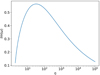 |
Fig. 6. Similar to Fig. 5 but for case F and a magnetized environment. |
| In the text | |
|
Fig. 7. Im(ω) versus magnetization σ for case F and a jet in a hydrodynamic environment. |
| In the text | |
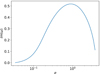 |
Fig. 8. Similar to Fig. 7 but for case F and a magnetized environment. |
| In the text | |
|
Fig. 9. Im(ω) versus the proper velocity of the outflow γυ for case F. The environment of the jet is hydrodynamic. The plot incorporates a secondary axis on the top edge of the plot box. The axis shows the proper fast magnetosonic Mach number. |
| In the text | |
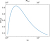 |
Fig. 10. Similar to Fig. 9 but for case F and a magnetized environment. |
| In the text | |
|
Fig. 11. Im(ω) versus the ratio between magnetic field components ϖ0 for case F. The jet is in a hydrodynamic environment. |
| In the text | |
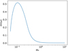 |
Fig. 12. Similar to Fig. 11 but for case F and a magnetized environment. |
| In the text | |
|
Fig. 13. Dispersion relation plot for KH mode (red colored solution) for the alternative configuration (case F5), for which the Lorentz factor γ = 5. |
| In the text | |
|
Fig. 14. Im(ω) versus density ratio η for the alternative configuration F5. The environment is hydrodynamic. |
| In the text | |
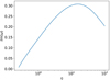 |
Fig. 15. Similar to Fig. 14 for case F5 and a magnetized environment. |
| In the text | |
|
Fig. 16. Im(ω) versus magnetization σ for the alternative configuration F5. The environment is hydrodynamic. |
| In the text | |
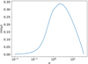 |
Fig. 17. Similar to Fig. 16 but for case F5 and a magnetized environment. |
| In the text | |
|
Fig. 18. Im(ω) versus the ratio of the magnetic field components ϖ0 for the alternative configuration F5. The environment is hydrodynamic. |
| In the text | |
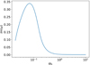 |
Fig. 19. Similar to Fig. 18 but for case F5 and a magnetized environment. |
| In the text | |
|
Fig. 20. Eigenfunctions in case F. The top plot shows y1 and the bottom plot shows y2. Solid and dashed lines represent the real and the imaginary part of the eigenfunctions. |
| In the text | |
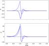 |
Fig. 21. Similar to Fig. 20 but for case F and k = 10. |
| In the text | |
|
Fig. 22. Eigenfunctions for alternative configuration F5. The top and bottom plots correspond to y1 and y2, respectively. Solid and dashed lines represent the real and the imaginary part of the eigenfunctions. |
| In the text | |
|
Fig. 23. Im(ω) versus density ratio η for the fiducial case F with a hydrodynamic environment. This plot compares results from the WKBJ approximation and the full numerical methodology. The WKBJ solution is depicted with blue solid lines and the numerical results are depicted with the orange dashed lines. |
| In the text | |
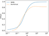 |
Fig. 24. Similar to Fig. 23 (case F) but for Im(ω) versus magnetization σ. |
| In the text | |
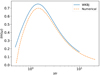 |
Fig. 25. Similar to Fig. 23 (case F) but for Im(ω) versus proper velocity γυ. |
| In the text | |
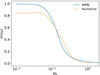 |
Fig. 26. Similar to Fig. 23 (case F) but for Im(ω) versus the ratio of magnetic field components ϖ0. |
| In the text | |
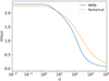 |
Fig. 27. Similar to Fig. 23 but for case F and k = 10. |
| In the text | |
|
Fig. 28. Im(ω)/k versus σ for case F. The jet is surrounded by a hydrodynamic environment. The solid line represents the solution in Cartesian geometry and the dashed lines show the solution in cylindrical geometry for k = π, 10. |
| In the text | |
|
Fig. 29. Im(ω)/k versus σ for case F. The jet is surrounded by a hydrodynamic environment. The solid line represents the solution in a Cartesian geometry and the dashed line represents that in a cylindrical geometry for k = π, 10. |
| In the text | |
|
Fig. 30. Im(ω)/k versus η for case F. The jet is surrounded by a hydrodynamic environment. The solid line represents the solution in a Cartesian geometry and the dashed line shows that in a cylindrical geometry for k = π, 10, 15. |
| In the text | |
Current usage metrics show cumulative count of Article Views (full-text article views including HTML views, PDF and ePub downloads, according to the available data) and Abstracts Views on Vision4Press platform.
Data correspond to usage on the plateform after 2015. The current usage metrics is available 48-96 hours after online publication and is updated daily on week days.
Initial download of the metrics may take a while.