| Issue |
A&A
Volume 680, December 2023
|
|
|---|---|---|
| Article Number | A65 | |
| Number of page(s) | 8 | |
| Section | Atomic, molecular, and nuclear data | |
| DOI | https://doi.org/10.1051/0004-6361/202346347 | |
| Published online | 08 December 2023 | |
Infrared spectra of TiO2 clusters for hot Jupiter atmospheres
1
Space Research Institute, Austrian Academy of Sciences,
Schmiedlstrasse 6,
8042
Graz, Austria
e-mail: This email address is being protected from spambots. You need JavaScript enabled to view it.
2
Centre for Exoplanet Science, University of St Andrews,
North Haugh,
St Andrews,
KY169SS,
UK
3
SUPA, School of Physics & Astronomy, University of St Andrews,
North Haugh,
St Andrews,
KY169SS,
UK
4
Institute for Astronomy, KU Leuven,
Celestijnenlaan 200D,
3001
Leuven, Belgium
5
TU Graz, Fakultät für Mathematik, Physik und Geodäsie,
Petersgasse 16,
8010
Graz, Austria
6
Department of Chemistry and Molecular Biology, University of Gothenburg,
Kemigården 4,
412 96
Gothenburg, Sweden
Received:
7
March
2023
Accepted:
21
June
2023
Abstract
Context. Clouds appear to be an unavoidable phenomenon in cool and dense environments. Hence, their inclusion is a necessary part of explaining observations of exoplanet atmospheres, most recently those of WASP 96b with the James Webb Space Telescope (JWST). Understanding the formation of cloud condensation nuclei in non-terrestrial environments is therefore crucial in developing accurate models to interpret current and future observations.
Aims. The goal of the paper is to support observations with infrared spectra for (TiO2)N clusters to study cloud formation in exoplanet atmospheres.
Methods. We derived vibrational frequencies from quantum-chemical calculations for 123 (TiO2)-clusters and their isomers and we evaluated their line-broadening mechanisms. Cluster spectra were calculated for several atmospheric levels for two example exoplanet atmospheres (WASP 121b-like and WASP 96b-like) to identify possible spectral fingerprints for cloud formation.
Results. The rotational motion of clusters and the rotational transitions within them cause significant line broadening, so that individual vibrational lines are broadened beyond the spectral resolution of the medium-resolution mode of the JWST mid-infrared instrument (MIRI) at R = 3000. However, each individual cluster isomer exhibits a ‘fingerprint’ IR spectrum. In particular, larger (TiO2) clusters have distinctly different spectra from smaller clusters. The morning and evening terminator for the same planet can exhibit different total absorbances, due to the greater abundance of different cluster sizes.
Conclusions. The largest (TiO2) clusters are not necessarily the most abundant (TiO2) clusters in the high-altitude regions of ultra-hot Jupiters and the different cluster isomers do contribute to the local absorbance. Planets with a considerable day-night asymmetry will be most suitable in the search for (TiO2) cluster isomers with the goal of improving cloud formation modelling.
Key words: line: profiles / molecular data / planets and satellites: atmospheres / infrared: planetary systems
© The Authors 2023
 Open Access article, published by EDP Sciences, under the terms of the Creative Commons Attribution License (https://creativecommons.org/licenses/by/4.0), which permits unrestricted use, distribution, and reproduction in any medium, provided the original work is properly cited.
This article is published in open access under the Subscribe to Open model. This email address is being protected from spambots. You need JavaScript enabled to view it. to support open access publication.
1 Introduction
The presence of clouds has been inferred for many exoplanet atmospheres as an explanation for suppressed absorption features and overall flat spectra (Charbonneau et al. 2002; Pont et al. 2008; Kreidberg et al. 2014). For hot Jupiters, cloud models predict that cloud particles are primarily made of a mix of silicates and other metal oxides (Helling et al. 2008; Mollière et al. 2017). Silicate spectra exhibit a vibrational Si-O stretching feature at 10 µm (Hackwell et al. 1970). With the launch of JWST in December 2021 and its near infrared observation capabilities in NIRCam, NIRSpec, and MIRI, the near-infrared (NIR) wavelength range (λ = 0.6–5 µm for NIRCam and NIR-Spec and λ = 5–28 µm for MIRI) has become accessible for observations at medium spectral resolutions. Miles et al. (2023) provided the first direct detection of absorption around the 10 µm band and, thus, of silicate-based clouds in a planetary mass companion, while observing VHS 1256b with JWST’s NIR-Spec and MIRI’s MRS instruments. Observations released for the JWST initial science release target WASP 96b showed that clouds were needed to explain its spectral features. Additionally, models for future JWST targets such as WASP 121b or WASP 43b do already exist, predicting their cloud coverage or lack thereof (Helling et al. 2021). In order to quantify the impact of clouds on the chemistry and elemental abundances in exoplanet atmospheres, their formation processes need to be understood. Cloud particles condense from supersaturated gas on so-called cloud condensation nuclei (CCN). On gaseous exoplanets, these CCN need to be formed from the gas phase through a process called nucleation. This process is the first step in cloud formation and starts as soon as the densities of the nucleating species are high and the temperatures are low enough. During the nucleation process, differently sized small clusters or different isomers of the same-sized cluster of the CCN-forming species co-exist and it is unknown whether only one or all participate in the chemical path to a thermally stable CCN, which then triggers the formation of a cloud particle. These clusters may have distinct spectral fingerprints, different to both that of the monomer and the bulk. Finding such spectral fingerprints may put the cloud formation modelling for extrasolar planets on much more solid ground. The aim of this paper is therefore to provide harmonic vibrational spectra of these small clusters for the nucleating species Titanium dioxide (TiO2) to enable discoveries similar to the unexpected SO2 detection in WASP-39b with JWST (Rustamkulov et al. 2023). These spectra arise from excited vibrational states of the clusters and their isomers that have energies that correspond to wavelengths in the infra-red range that can be probed by JWST’s MIRI. Rotational transitions have energies in the millimetre wavelength ranges, but they also happen within vibrational state transitions, broadening the corresponding vibrational bands.
Section 2 describes how the harmonic vibrational spectra are extracted from quantum-chemical calculations performed in Sindel et al. (2022) and the broadening mechanisms considered. Section 3 compares the spectra for different clusters and isomers and presents the resulting total absorbance caused by (TiO2)N clusters for two exoplanet atmosphere models. In Sect. 4, we discuss our results and their limits. Section 5 summarises the paper and gives and outlook on possible future work.
Number of isomers for each cluster size, N.
2 Methods
2.1 Extraction of harmonic IR frequencies
This work investigates the infrared spectra of small (TiO2)N clusters. The harmonic vibrational spectra discussed in this work are based on the results of density functional theory (DFT) frequency calculations performed with the B3LYP functional (Becke 1993), cc-pVTZ basis-set (Wilson et al. 1996), and gd3bj empirical dispersion (Grimme et al. 2011). The cluster structure and energy calculations were presented in Sindel et al. (2022), for (TiO2)N clusters of sizes N = 1–15. For all clusters with sizes N > 1, multiple isomers were considered. (see Table 1). For each cluster size, N, there is one most energetically favourable cluster configuration, the so-called global minimum candidate (GM). The GM is given the suffix ‘-A’; for instance, TI6O12-A denotes the GM cluster of size 6. The second lowest-energy isomer, namely, the energetically next favourable cluster at T = 0K is given the suffix -B, the third -C, and so on.
The frequencies and their corresponding infrared (IR) intensities are given in units of [cm−1] and  , respectively. We note that some of the low-energy and high-wavelength modes (λ ≳ 77 µm) are not pure vibrational modes, but can arise from hindered rotation, where certain rotations of the molecule are inhibited due to its geometry. In this work, we treat all modes as purely harmonic vibrational modes. We converted the IR intensities to molar absorption coefficients according to Spanget-Larsen (2015). The unknown quantity for this transformation is the line-width for each active IR mode. To quantify the line-width several broadening mechanisms are evaluated for the physical parameter spaces of exoplanetary atmospheres.
2.1.1 Thermal broadening
The thermal broadening of a line is caused by the multidirectional movement of individual line-sources within a gas. The broadening in frequency (∆ν) by thermal broadening is dependent on the temperature (T), the frequency (ν), and the mass of the individual line-sources, namely, the cluster, (m) through:
 (1)
(1)
where kB is the Boltzmann constant and c is the speed of light. As a consequence, large and more massive clusters show smaller thermal line broadening than small clusters. Here, we assume that each active frequency mode ofaclusteris broadened equally.
2.1.2 Collisional broadening
In a dense gas, spontaneous emissions can typically be induced, that is, triggered prematurely through collisions with other particles. This shortens the average lifetime of the state and therefore increases the uncertainty in energy and thereby in frequency. The relative broadening at a frequency is given by
 (2)
(2)
where νcol is the frequency of collisions within the gas, which is given by the root mean square (RMS) velocity of the gas particles (υrms) and the mean free path (λ):
 (3)
(3)
with the RMS velocity of a gas being:
 (4)
(4)
with the ideal gas constant, R, the gas temperature, T, and the mean molecular weight of the gas, M. The mean free path is given as:
 (5)
(5)
with the gas pressure, p, the effective cross-section of the cluster, σ, and the Avogadro constant, NA.
2.1.3 Rotational broadening
A molecule with n atoms has 3n − 6 vibrational modes. The rotational motion of the molecule can affect the vibrational motion and vice versa. This means that the vibrational energy levels are slightly dependent on the rotational energy levels. As a result, when rotational transitions occur, they can slightly shift the vibrational energy levels, which then leads to additional broadening of the vibrational spectral lines. The population of rotational states J follows a Boltzmann distribution. In order to quantify the broadening mechanism induced by these rotational states, the maximum rotational quantum number Jmax is used. It is defined by:
 (6)
(6)
Here, B is the rotational constant of the molecule and defines the spacing of rotational energy levels. This maximum rotational quantum number specifies the most likely occupied rotational energy state (Hollas 2002). Since the broadening effect is symmetric, the frequency space spanned by the rotational states from J = 0 to Jmax is taken as the FWHM for our broadening approximation. The broadening induced by this process is therefore given as:
 (7)
(7)
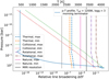 |
Fig. 1 Comparison of the considered broadening mechanisms along a (pgas, Tgas) profile. All broadening mechanisms are evaluated for their potential minimum and maximum contribution. Thermal broadening is weakest for large clusters (N = 15, ‘Thermal, min’) and strongest for small clusters (N = 1, ‘Thermal, max’). Collisional broadening is weakest for small clusters at high frequencies (N = 1, λ = 10 µm, ‘Collisional, min’) and strongest for large clusters at low frequencies (N = 15, λ = 100 µm, ‘Collisional, max’). Rotational broadening is weakest for large clusters (N = 15, ‘Rotational, min’) and strongest for small clusters (N = 1, ‘Rotational, max’). Natural broadening is weakest for long state life-times at high frequency (τ = 1µs, λ = 10 µm, ‘Natural, min’) and strongest for short state life-times at low frequency (τ = 1ns, λ = 100 µm, ‘Natural, max’). The T(p) profile is one of the WASP-96b-like profiles from Sect. 2.3. |
2.1.4 Natural broadening
Natural broadening occurs due to the Heisenberg uncertainty principle. An uncertainty in the life-time of an excited state (∆t) leads to an uncertainty in its energy (∆E) and, thus, in in its frequency (∆ν), as follows:
 (8)
(8)
Natural broadening effects are usually small when compared to other broadening effects (Fig. 1), so they are not considered in this work.
2.2 Number densities of (TiO2)N clusters
To calculate not only the relative molar absorbances of the individual (TiO2)N clusters at different pressure and temperature points, but the absolute absorbance of each species at certain pressure levels in the atmosphere as well, number densities for as many species as possible need to be included, because they all contribute differently to the overall absorption. In order to achieve this, we input the thermochemical cluster-data into the equilibrium chemistry code GGCHEM Woitke et al. (2018). The molecular equilibrium constants are fit using the approach from Stock et al. (2018). The Gibbs free energies of the formation  are calculated via:
 (9)
(9)
Values for  are taken from Sindel et al. (2022), while
  for Ti and O are taken from the JANAF-NIST thermochemical tables (Chase 1998). The resulting fit for the kp values is then done via Eqs. (13) and (17) in Woitke et al. (2018), which are thus combined as follows:
 (10)
(10)
with the fit-coefficients a0, a1, b0, b1, and b2. These are then implemented into GGCHEM for the 123 considered (TiO2)N cluster isomers (see Table 1), enabling the calculation of their number densities from equilibrium chemistry at any pressure temperature point with T > 100 K.
2.3 Atmospheric pressure – temperature profiles
We use 1D pressure-temperature (pgas, Tgas) profiles that were extracted from Baeyens et al. (2021) and extended to pressures of 10−15 bar. We focus on two specific cases: a WASP-121b-like planet (T* = 6500 K, Teff = 2200 K, log(g) = 3) and a WASP-96b like planet (T* = 5650 K, Teff = 1200 K, log(g) = 3). WASP 96b is a puffy hot Jupiter that is cold enough to produce cloud coverage everywhere but the substellar point, and the existence of clouds has been predicted by cloud formation models (Samra et al. 2023). WASP 121b is an ultra-hot Jupiter with extremely high dayside-nightside temperature differences, whereby clouds are only expected to form on the nightside (Helling et al. 2021). For both of the planets a (pgas, Tgas) profile for the morning and the evening terminator were used.
2.4 Absorbance of clusters
For all of the (pgas, Tgas)-profiles, we started from a gas of solar composition (Asplund et al. 2009) and ran GGCHEM for gasphase species only at every point along the (pgas, Tgas)-curve. This provides the number densities for all isomers. At each pressure and temperature point, all broadening mechanisms are evaluated for all vibrational lines of all clusters and the strongest broadening mechanism is chosen. The broadening through this method is used as the input broadening width, w, to convert the lines IR intensity into an absorption profile, σ, with units of [cm2/molecule]. All absorption profiles are mutliplied by the number density ![Mathematical equation: $\left[ {{{{\rm{molecule}}} \over {{\rm{c}}{{\rm{m}}^{\rm{3}}}}}} \right]$](/articles/aa/full_html/2023/12/aa46347-23/aa46347-23-eq15.png) of their respective cluster, giving their total absorbance Atot in
of their respective cluster, giving their total absorbance Atot in ![Mathematical equation: $\left[ {{{\rm{1}} \over {{\rm{cm}}}}} \right]$](/articles/aa/full_html/2023/12/aa46347-23/aa46347-23-eq16.png) as follows:
as follows:
 (11)
(11)
3 Results
3.1 Broadening mechanisms
The impact of the broadening mechanisms at different pressure levels at the morning-side terminator of a WASP-96b like planet is investigated here as an example (Fig. 1). The point of interest here is whether the individual vibrational modes could possibly be resolved by JWSTs MIRI instrument at its working spectral resolution of R ~ 3000. Any mechanisms that would broaden the lines further than that would also make them resolvable at this resolution.
The impact of collisional broadening significantly depends on the pressure. In our test case atmosphere, it is only relevant at high pressures low in the atmosphere. For the atmosphere used in this test case, the upper layers are largely isothermal. Therefore, the broadening mechanisms that depend predominantly on temperature such as thermal and rotational broadening are constant throughout most of the atmosphere and only change when the temperature changes as well. For natural broadening, the smallest broadening effects are characterised by a long state life-time and a small emission wavelength (see Eq. (8)). Here, τ = 1µs and λ = 10 µm are chosen as representative values. The maximum broadening scenario corresponds to a short state life-time (τ = 1ns) and a large emission wavelength (λ = 100 µm). In both cases, the relative line broadening is far below the rotational broadening. Therefore, the choice to neglect natural broadening is justified. The most impactful broadening mechanism throughout most of the atmosphere is rotational broadening, dominating everywhere but deep in the atmosphere.
3.2 Raw spectra of (TiO2)N clusters
Every (TiO2)N cluster contains X = 3N atoms and shows 3X − 6 vibrational modes. Therefore, the overall opacity is expected to increase with the cluster size, N. Wavelength-dependent cross-sections, ![Mathematical equation: ${\sigma _{{\rm{cluster}}}}\left( \lambda \right)\left[ {{{{\rm{c}}{{\rm{m}}^{\rm{2}}}} \over {{\rm{molecule}}}}} \right]$](/articles/aa/full_html/2023/12/aa46347-23/aa46347-23-eq18.png) , were computed for 123 isomers of sizes N = 1–15 of the (TiO2)N clusters. The broadening for each line at a temperature of T = 1000 K and a pressure of p = 1 bar was calculated and the lines broadened according to Spanget-Larsen (2015): each line profile is given by a Lorentzian with a FWHM of w and a maximum of
, were computed for 123 isomers of sizes N = 1–15 of the (TiO2)N clusters. The broadening for each line at a temperature of T = 1000 K and a pressure of p = 1 bar was calculated and the lines broadened according to Spanget-Larsen (2015): each line profile is given by a Lorentzian with a FWHM of w and a maximum of  . The width, w was computed by comparing the broadening mechanisms (discussed in Sect. 2.1) and using the width produced by the dominant one. A comparison to show trends between different sizes is shown in Fig. 2. In the whole spectral range of λ = 5–100 µm cross-sections of larger clusters tend to be larger than ones of smaller clusters. Especially in the wavelength-range observed by the JWST/MIRI instrument of 5–28 µm, larger clusters are stronger absorbers than smaller clusters, while the TiO2 monomer has no significant absorption cross-section over most of this range. Cluster growth (i.e. nucleation) will therefore lead to an increase of absorption in the ~4–25 µm wavelength region, with the largest clusters dominating the absorption.
Generally, not only the GM cluster will be present, but energetically less favourable isomers will also be present in the atmosphere. Since their geometries are different, their vibrational spectra also differ. A comparison is made of cross-sections for the three isomers of the size N = 2 (Fig. 3) and the four lowest-energy isomers of size N = 15 (Fig. 4).
For the molecular cross-sections of a small cluster, (TiO2)2, there are differences between the isomers, especially for wavelengths towards the tail at 100 µm. Within the MIRI wavelength range (5–28 µm), they agree in terms of the key features, such as the peak being just short of ~10 µm and the double peak at ~15 µm for the two most favourable isomers. For the large cluster (TiO2)15, the forest of lines at shorter wavelengths covering most of the MIRI wavelength range can only be disentangled at high spectral resolutions. At longer wavelengths, differences in line positions become clearer. It is important to note that all four energetically favourable isomers share a strong line feature at ~10 µm.
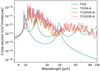 |
Fig. 2 Wavelength-dependent cross-sections, σduster(λ), for the GM clusters for sizes of N = 1, 2, 10, 15. |
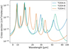 |
Fig. 3 Wavelength-dependent cross-sections, σcluster(λ), for all three isomers of the (TiO2)2 cluster. |
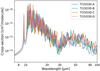 |
Fig. 4 Wavelength-dependent cross-sections, σcluster(λ), for the four energetically most favourable isomers of the (TiO2)15 cluster. |
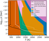 |
Fig. 5 Most abundant Ti-containing species in chemical equilibrium at solar metallicity as a function of temperature and pressure. Letters after clusters indicate energetic isomer ordering within isomers of the same size, i.e. -A indicates the GM isomer, while -B would indicate the second most energetically favourable isomer. Temperature pressure profiles for morning (in black) and evening (in white) terminators of a WASP 96b-like planet and a WASP 121b-Hke extrasolar planet are over-plotted. |
3.3 Cluster number densities in chemical equilibrium
To calculate the total absorbance of a species, the cross-sections for each isomer of each cluster need to be multiplied by their respective number density in the atmosphere. The chemical equilibrium code GGCHEM is used to compute the number densities of all Ti-bearing molecules and clusters from solar metallicity in a grid of pressures from p = 10−15−700 bar and temperatures of T = 300–3000 K (Fig. 5). On the WASP 96b-like planet (solid lines in Fig. 5), the cluster composition in the upper atmosphere is dominated by the largest cluster resulting from the calculations (TiO2)15 for both terminators. It is reasonable to assume that larger clusters would be more favourable if they were included in the calculations. In the lower atmosphere between ~ 1–100 bar, the largest cluster is no longer the most favoured Ti-bearing compound and, instead, the second-largest cluster, (TiO2)14 is more abundant. At these pressure levels, a limit to the stability of larger clusters has been reached, making the smaller cluster more favourable. For the WASP 121b-like planet (dotted lines), the terminators probe different conditions leading to different atmospheric compositions. At the top of the atmosphere at the morning terminator, the TiO2 monomer is dominant, as any larger clusters are less favourable at these temperatures and pressures. This tendency changes when moving downwards in the atmosphere, as the pressure increases and, thus, the densities of the atmosphere increase as well. At pressures between ~10−11−10−6 bar, some growth of clusters is favoured, again leaving the second largest cluster (TiO2)14 as the most abundant one. As pressures further increase, namely, deeper in the atmosphere, larger clusters, represented by (TiO2)15 in this work, become the most favourable species (pgas ≈ 10−6−10−1 bar), after which the temperature increases beyond the stability limit and follows a similar path to the terminators of the WASP 96b-like planet. The hotter evening terminator starts within the TiO-dominated regime, where temperatures are high enough for the smaller molecule to be favoured over the TiO2 monomer. This dominance continues down to p ~ 10−5 bar, interrupted by a small section (~10−13−10−11 bar) where TiO2 is most abundant. Larger clusters (N ≥ 15) are never favoured along this terminator and only the (TiO2)14 cluster is most abundant between p ≈ 10−5−10−2 bar. Deep in the atmosphere, where temperatures are higher, the titanium content is dominated by first the more thermally stable TiO and at higher pressures, it is instead the atomic Ti. A slice through this graph at p = 10−8 bar showcases the prevalence of different clusters at different temperatures (Fig. 6). For temperatures of T < 600 K, the GM candidate of the largest cluster, (TiO2)is, is the only relevant Ti-bearing species. As the temperature rises, the second largest cluster (TiO2)14 rises in abundance, indicating a comparatively enhanced preference at certain temperatures and pressures, as it becomes the most abundant species at T ≈ 1100 K. In the region between ~900–1300 K, low abundances of many intermediate sized GM clusters and their respective metastable isomers can be seen. In particular, the size N = 12 cluster (solid gold) and the N = 2 cluster (solid red) play a role in such cases. The relative energies between isomers of the same size vary with temperature, so that different isomers may become the most abundant of their size at different temperature points. For N = 15, the energy difference of isomers A and B at 300 K is  . At 1500 K, this difference decreases to
  . At 3000 K, isomer B is more energetically favourable, as the difference is
  . The first isomer of N = 15 that does not reach the cut-off concentration of
  is TI15O30-D. The relative energy to the most stable N = 15 isomer is always
  across the entire temperature range 300–3000 K. The relative cut-off energy is therefore at around
  for N = 15.
As the temperature increases beyond the stability for clusters, the abundance of the TiO2 monomer rises. The difference in peak abundance between TiO2 and (TiO2)15 is about an order of magnitude, indicating that a similar amount of Ti and O is used to produce these concentrations.
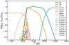 |
Fig. 6 Concentration of Ti-bearing gas-phase species across a temperature range of 300–3000 K. Letters after cluster names indicate different isomers, with -A being the energetically most favourable (GM) isomer. Only species that reach a concentration of |

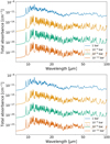 |
Fig. 7 Total absorbance from (TiO2)N clusters at different pressure levels of a WASP 96b-like exoplanet atmosphere as a function of the wavelength. Top: morning terminator. Bottom: evening terminator. |
3.4 Spectra at different atmospheric pressure levels
To investigate the change of the absorption profiles of (TiO2)N clusters at different pressure levels in the atmosphere, the spectra are computed at even logarithmic steps from p = 10−15−102 bar. At each pressure level, GGCHEM is run to obtain the number densities of all considered species, that is, the 576 atoms and molecules included in GGCHEM as well as the 123 clusters from this work. As the molecular cross-sections span no more than five orders of magnitude, contributions from clusters with abundances that are more than five magnitudes lower than the most abundant cluster are neglected to save on the computational cost of the absorbance calculation. For each of the remaining species, the absorbance is calculated by multiplying the molecular cross-section with its number density. All absorbances are then added up to the total absorbance of (TiO2)N clusters at the given pressure level.
For the WASP 96b-like planet (Fig. 7), there are only minor differences between the morning and evening terminator, owing to the fact that both temperature-pressure profile occupy similar regions in the phase-diagram (Fig. 5). At the bottom of the atmosphere at 1 bar, there are many cluster sizes and their isomers contributing to the total spectrum, which end up blending lines and causing the lack of distinct peaks towards the longer-wavelength part of the spectrum. Additionally, the higher pressure causes more collisional broadening, further blending the lines. This situation changes when moving upwards in the atmosphere, where the Ti content is dominated by the large cluster (TiO2)15, with its distinct lines across the wavelength range. The most visible difference between the morning and evening terminators are the small peaks at ~10 and 12 µm that exist for the evening terminator, but not for the morning terminator. As the evening terminator is hotter, (TiO2)15 becomes less favourable and some contribution from the next smaller cluster is visible, as these peaks are caused by absorption from (TiO2)14. One overall trend seen here is that the absorbance is higher at higher pressures, namely, lower in the atmosphere. This is due to the fact that number densities are much higher at the bottom of the atmosphere.
The spectra for the WASP 121b-like planet (Fig. 8) are more easily distinguishable with respect to their terminators. At the evening terminator, the only contributing TÍO2 species is the monomer for low pressures levels (p = 10−12, 10−8 bar) and high pressure levels (p = 1 bar). The TiO molecule is the dominant Ti-bearing species for most high and low pressures (p < 10−6 bar and p > 10−2 bar). Only at an intermediate pressure level (p = 10−4 bar) clusters may contribute to the spectrum. As the second largest cluster (TiO2)14 is the most abundant here, the peaks at 10 and 12 µm are well pronounced. It also showcases the strength of absorption of larger clusters in comparison to the monomer, as the total absorbance with the contribution of the clusters approaches, and sometimes exceeds, the absorbance of the monomer at much higher pressures. For the morning terminator, only the upper atmosphere is dominated by the TiO2 monomer. Lower in the atmosphere, the spectra have contributions from many clusters and isomers, as both (TiO2)14 and (TiO2)15 and its isomers are highly abundant. At the bottom of the atmosphere (p = 1 bar), fewer isomers and clusters are present due to the higher temperature, leading to less distinct lines, as well as the higher collisional broadening causing the lines to blend into each other.
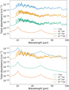 |
Fig. 8 Total absorbance from (TiO2)N clusters at different pressure levels of a WASP 121b-like exoplanet atmosphere as a function of the wavelength. Top: morning terminator. Bottom: evening terminator. |
4 Discussion
The (TiO2)N clusters considered in this work extend to a maximum size of N = 15. As the largest cluster is the most abundant one, covering a large area of the parameter space (Fig. 5), this has certain implications for our results. When the largest considered cluster is also the most abundant one, the larger clusters, which are more stable when extrapolating observed trends, are likely to be more abundant. It is therefore important to note that the spectra at pressure levels in the (pgas, Tgas)-profiles where (TiO2)15 is the most abundant species are likely to also contain contributions from even larger clusters or the bulk-phase of TiO2. A general point can be made about the differences of the spectra of different cluster sizes. The absorption cross-sections of larger clusters exhibit a denser forest of stronger lines at shorter wavelengths and more distinct lines at longer wavelengths (Fig. 2), when compared to the absorption cross-sections of smaller clusters.
Additionally there are areas in the (pgas, Tgas) parameter space where it is not, in fact, the largest, but the second-largest cluster that is the most energetically favourable (green area in Fig. 5, ~1000 K at 10−12 bar and ~1200–2000 K at 103 bar). Figure 6 shows that also smaller cluster sizes have significant abundances. If this trend continues, not all areas of the parameter space that are dominated by (TiO2)15 (approximately <1000 K at all pressures) in this work are necessarily dominated by larger clusters when taken into consideration. Another caveat of the spectra produced in this work originates from the harmonic oscillator approximation to the vibrational modes of the individual clusters. Guiu et al. (2021) have shown that anhar-monicities and non-uniform thermal effects in the vibrational modes have an impact on line position and strength, already at low temperatures. However, treating all frequency calculations at a full anharmonic level is prohibitively computationally expensive with respect to the scope of this paper. General trends of line intensity or line density increasing with cluster size are not impacted by anharmonicities, which allows for qualitative statements to be made on the resulting spectra.
This work shows that it is possible to distinguish between the absorption caused by the TiO2 monomer and any (TiO2)N clusters with N > 1 , as the absorption cross-sections at wavelengths λ ~ 12–25 µm are up to three orders of magnitudes larger for clusters than they are for the monomer. Detections of such an absorption feature with, for instance, JWST/MIRI could indicate the presence of TiO2 clusters and confirm their role in the formation of cloud condensation nuclei for cloud formation. This work shows the areas in the investigated atmospheres where (TiO2)N clusters play the role of absorbing species. Other absorbing species could play a larger role or, in the case of the presence of clouds, the atmosphere can become optically thick above the pressure levels where the clusters contribute to the total absorbance. Silicate clouds have a feature around 10 µm (Wakeford & Sing 2015), which is in the vicinity of the shared ~9.5 µm feature of the clusters from this work. The clusters could therefore explain the existence of a 10 micron feature in the absence of clouds. We note that beside (TiO2)N, N = 1–15, other metal oxide clusters also exhibit their most intense emissions between 9.5 and 12.5 µm, including clusters of silicates (Zamirri et al. 2019) and alumina (Gobrecht et al. 2022). This might represent an additional challenge in identifying and discriminating the cluster species and sizes by IR spectroscopy. The most interesting (pgas, Tgas) points to probe are the ones contained in the green area in Fig. 5, where (TiO2)14 is the most abundant species, as cluster growth towards larger clusters and the solid phase is inhibited in these regions, but medium-sized clusters have already formed and are contributing to absorption with denser and stronger cross-sections. These pressures and temperatures can be probed in the upper atmosphere of a WASP 121b-like exoplanet (black dashed line in Fig. 5).
5 Conclusions
This work demonstrates that (TiO2)N clusters have unique vibrational absorption spectra. When considering broadening mechanisms of the individual vibrational modes, the lines are broadened beyond JWST/MIRI spectral resolution throughout most of the atmosphere of these exoplanet examples. There are clear differences between the spectra of smaller and larger clusters, as increasing size is correlated with more lines overall, as well as denser lines at shorter wavelengths and an overall higher cross-section. Different cluster isomers of the same size have different line positions and intensities, while trends in the cross-section demonstrate, for instance, higher cross-sections towards shorter wavelengths. Different cluster sizes dominate different areas of the pressure-temperature parameter space (Fig. 5), including isomers differing from the GM candidate dominating the spectra at different points in the studied exoplanet atmospheres. For the WASP 96b-like atmosphere, there is a small difference between the morning and evening terminator spectra that is due to a higher relative abundance of the (TiO2)14 cluster in the latter. For the WASP 121b-like planet, the upper atmosphere is always dominated by the TiO2 monomer and the TiO molecule, offering a possible clue as to how deeply the atmosphere is probed. When it comes to detecting the building blocks that are relevant for cloud formation on their way to becoming CCN, the atmosphere of an ultra-hot Jupiter such as WASP 121b is better suited for the search, as compared to a WASP 96b-like planet.
These model spectra of TiO2 clusters can be implemented into radiative transfer models of exoplanet atmospheres to gauge whether their detection with modern instruments is possible. This potential detection or non-detection of the specific fingerprints of the individual clusters could give an indication towards the formation of the clusters and their role as CCN in these exoplanet atmospheres. When used with observational data, however, the caveats need to be addressed. The harmonic oscillator approximation used in this work provides a useful and effective means of analysing vibrational spectra. More complex descriptions that would include the anharmonicities, ro-vibrational coupling, and non-uniform thermal effects would improve the precision of line positions, but they come at much higher computational cost. The changes in line position induced by these effects are small enough (Guiu et al. (2021) found line shifts of a few percent at wavelengths λ ~ 10 µm) to be blurred out at low spectral resolutions, for instance, MIRI’s LR mode. Treating these effects would make these data useful for MIRI’s medium spectral resolution. The templates provided in this paper can be used to model the absorption caused by these CCN-forming clusters at lower spectral resolutions.
Acknowledgements
J.P.S. acknowledges a St Leonard’s Global Doctoral Scholarship from the University of St Andrews and funding from the Austrian Academy of Science. Ch.H. and L.D. acknowledge funding from the European Union H2020-MSCA-ITN-2019 under Grant Agreement no. 860470 (CHAMELEON). D.G. acknowledges funding by the project grant “The Origin and Fate of Dust in Our Universe” from the Knut and Alice Wallenberg Foundation (KAW 2020.0081).
References
- Asplund, M., Grevesse, N., Sauval, A. J., & Scott, P. 2009, ARA&A, 47, 481 [NASA ADS] [CrossRef] [Google Scholar]
- Baeyens, R., Decin, L., Carone, L., et al. 2021, MNRAS, 505, 5603 [NASA ADS] [CrossRef] [Google Scholar]
- Becke, A. D. 1993, J. Chem. Phys., 98, 5648 [Google Scholar]
- Charbonneau, D., Brown, T. M., Noyes, R. W., & Gilliland, R. L. 2002, ApJ, 568, 377 [Google Scholar]
- Gobrecht, D., Plane, J. M., Bromley, S. T., et al. 2022, A&A, 658, A167 [NASA ADS] [CrossRef] [EDP Sciences] [Google Scholar]
- Grimme, S., Ehrlich, S., & Goerigk, L. 2011, J. Comput. Chem., 32, 1456 [Google Scholar]
- Guiu, J. M., Escatllar, A. M., & Bromley, S. T. 2021, ACS Earth Space Chem., 5, 812 [NASA ADS] [CrossRef] [Google Scholar]
- Hackwell, J. A., Gehrz, R. D., & Woolf, N. J. 1970, Nature, 227, 822 [NASA ADS] [CrossRef] [Google Scholar]
- Helling, C., Woitke, P., & Thi, W. F. 2008, A&A, 485, 547 [NASA ADS] [CrossRef] [EDP Sciences] [Google Scholar]
- Helling, C., Lewis, D., Samra, D., et al. 2021, A&A, 649, A44 [NASA ADS] [CrossRef] [EDP Sciences] [Google Scholar]
- Hollas, J. M. 2002, Basic Atomic and Molecular Spectroscopy (The Royal Society of Chemistry) (Hoboken: Wiley) [CrossRef] [Google Scholar]
- Kreidberg, L., Bean, J. L., Désert, J. M., et al. 2014, Nature, 505, 69 [NASA ADS] [CrossRef] [Google Scholar]
- Chase, M. W., 1998, NIST-JANAF Thermochemical Tables, 4th edn. (American Institute of Physics) [Google Scholar]
- Miles, B. E., Biller, B. A., Patapis, P., et al. 2023, ApJ, 946, L6 [NASA ADS] [CrossRef] [Google Scholar]
- Mollière, P., Van Boekel, R., Bouwman, J., et al. 2017, A&A, 600, A10 [CrossRef] [EDP Sciences] [Google Scholar]
- Pont, F., Knutson, H., Gilliland, R. L., Moutou, C., & Charbonneau, D. 2008, MNRAS, 385, 109 [Google Scholar]
- Rustamkulov, Z., Sing, D., Mukherjee, S., et al. 2023, AAS, 55, 124.01 [NASA ADS] [Google Scholar]
- Samra, D., Helling, C., Chubb, K. L., et al. 2023, A&A, 669, A142 [NASA ADS] [CrossRef] [EDP Sciences] [Google Scholar]
- Sindel, J. P., Gobrecht, D., Helling, C., & Decin, L. 2022, A&A, 668, A35 [NASA ADS] [CrossRef] [EDP Sciences] [Google Scholar]
- Spanget-Larsen, J. 2015, IR intensity and Lorentz epsilon curve form ‘Gaussian’ FREQ output, https://doi.org/10.13140/RG.2.1.4181.6160 [Google Scholar]
- Stock, J. W., Kitzmann, D., Patzer, A. B. C., & Sedlmayr, E. 2018, MNRAS, 479, 865 [NASA ADS] [Google Scholar]
- Wakeford, H. R., & Sing, D. K. 2015, A&A, 573, A122 [NASA ADS] [CrossRef] [EDP Sciences] [Google Scholar]
- Wilson, A. K., Van Mourik, T., & Dunning, T. H. 1996, J. Mol. Struc. THEOCHEM, 388, 339 [CrossRef] [Google Scholar]
- Woitke, P., Helling, C., Hunter, G. H., et al. 2018, A&A, 614, A1 [NASA ADS] [CrossRef] [EDP Sciences] [Google Scholar]
- Zamirri, L., MacIà Escatllar, A., Marinõso Guiu, J., Ugliengo, P., & Bromley, S. T. 2019, ACS Earth Space Chemistry, 3, 2323 [NASA ADS] [CrossRef] [Google Scholar]
All Tables
All Figures
|
Fig. 1 Comparison of the considered broadening mechanisms along a (pgas, Tgas) profile. All broadening mechanisms are evaluated for their potential minimum and maximum contribution. Thermal broadening is weakest for large clusters (N = 15, ‘Thermal, min’) and strongest for small clusters (N = 1, ‘Thermal, max’). Collisional broadening is weakest for small clusters at high frequencies (N = 1, λ = 10 µm, ‘Collisional, min’) and strongest for large clusters at low frequencies (N = 15, λ = 100 µm, ‘Collisional, max’). Rotational broadening is weakest for large clusters (N = 15, ‘Rotational, min’) and strongest for small clusters (N = 1, ‘Rotational, max’). Natural broadening is weakest for long state life-times at high frequency (τ = 1µs, λ = 10 µm, ‘Natural, min’) and strongest for short state life-times at low frequency (τ = 1ns, λ = 100 µm, ‘Natural, max’). The T(p) profile is one of the WASP-96b-like profiles from Sect. 2.3. |
| In the text | |
|
Fig. 2 Wavelength-dependent cross-sections, σduster(λ), for the GM clusters for sizes of N = 1, 2, 10, 15. |
| In the text | |
|
Fig. 3 Wavelength-dependent cross-sections, σcluster(λ), for all three isomers of the (TiO2)2 cluster. |
| In the text | |
|
Fig. 4 Wavelength-dependent cross-sections, σcluster(λ), for the four energetically most favourable isomers of the (TiO2)15 cluster. |
| In the text | |
|
Fig. 5 Most abundant Ti-containing species in chemical equilibrium at solar metallicity as a function of temperature and pressure. Letters after clusters indicate energetic isomer ordering within isomers of the same size, i.e. -A indicates the GM isomer, while -B would indicate the second most energetically favourable isomer. Temperature pressure profiles for morning (in black) and evening (in white) terminators of a WASP 96b-like planet and a WASP 121b-Hke extrasolar planet are over-plotted. |
| In the text | |
|
Fig. 6 Concentration of Ti-bearing gas-phase species across a temperature range of 300–3000 K. Letters after cluster names indicate different isomers, with -A being the energetically most favourable (GM) isomer. Only species that reach a concentration of |
| In the text | |
|
Fig. 7 Total absorbance from (TiO2)N clusters at different pressure levels of a WASP 96b-like exoplanet atmosphere as a function of the wavelength. Top: morning terminator. Bottom: evening terminator. |
| In the text | |
|
Fig. 8 Total absorbance from (TiO2)N clusters at different pressure levels of a WASP 121b-like exoplanet atmosphere as a function of the wavelength. Top: morning terminator. Bottom: evening terminator. |
| In the text | |
Current usage metrics show cumulative count of Article Views (full-text article views including HTML views, PDF and ePub downloads, according to the available data) and Abstracts Views on Vision4Press platform.
Data correspond to usage on the plateform after 2015. The current usage metrics is available 48-96 hours after online publication and is updated daily on week days.
Initial download of the metrics may take a while.