| Issue |
A&A
Volume 679, November 2023
|
|
|---|---|---|
| Article Number | A113 | |
| Number of page(s) | 10 | |
| Section | Stellar structure and evolution | |
| DOI | https://doi.org/10.1051/0004-6361/202347496 | |
| Published online | 29 November 2023 | |
Influence of the tetraneutron on the EoS under core-collapse supernova and heavy-ion collision conditions
1
Department of Fundamental Physics, University of Salamanca, 37008 Salamanca, Spain
e-mail: This email address is being protected from spambots. You need JavaScript enabled to view it.
2
CFisUC, University of Coimbra, 3004-516 Coimbra, Portugal
Received:
18
July
2023
Accepted:
20
September
2023
Abstract
Context. Recently, a resonant state of four neutrons (tetraneutron) with an energy of E4n = 2.37 ± 0.38(stat) ± 0.44(sys) MeV and a width of Γ = 1.75 ± 0.22(stat) ± 0.30(sys) MeV was reported.
Aims. In this work, we analyze the effect of including such an exotic state on the yields of other light clusters; these clusters not only form in astrophysical sites, such as core-collapse supernovae and neutron star (NS) mergers, but also in heavy-ion collisions.
Methods. To this aim, we used a relativistic mean-field (RMF) formalism, where we consider in-medium effects in a two-fold way – that is, via the couplings of the clusters to the mesons, and via a binding energy shift – to compute the low-density equation of state (EoS) for nuclear matter at finite temperature and fixed proton fraction. We consider five light clusters – namely deuterons, tritons, helions, α-particles, and 6He – immersed in a gas of protons and neutrons, and we calculate their abundances and chemical equilibrium constants with and without the tetraneutron. We also analyze how the associated energy of the tetraneutron would influence such results.
Results. We find that the low-temperature, neutron-rich systems are the ones most affected by the presence of the tetraneutron, making NSs excellent environments for their formation. Moreover, its presence in strongly asymmetric matter may increase the proton and α-particle fractions considerably. This may have an influence on the dissolution of the accretion disk of the merger of two NSs.
Key words: stars: neutron / equation of state / dense matter / nuclear reactions / nucleosynthesis / abundances
© The Authors 2023
 Open Access article, published by EDP Sciences, under the terms of the Creative Commons Attribution License (https://creativecommons.org/licenses/by/4.0), which permits unrestricted use, distribution, and reproduction in any medium, provided the original work is properly cited.
This article is published in open access under the Subscribe to Open model. This email address is being protected from spambots. You need JavaScript enabled to view it. to support open access publication.
1. Introduction
For decades, experimentalists have been trying to find a resonant or bound state constituted by four neutrons. Following an experiment at RIKEN with the SAMURAI spectrometer, using a high-energy beam of 8He on a proton target, Duer et al. (2022) reported the production of a resonant state of four neutrons with an energy of E4n = 2.37 ± 0.38(stat) ± 0.44(sys) MeV and a width of Γ = 1.75 ± 0.22(stat) ± 0.30(sys) MeV. This value for the energy is substantially higher (and the width lower) than found in a previous experiment (Kisamori et al. 2016), where a high-energy radioactive 8He beam was used to hit a liquid 4He target, producing a resonant tetraneutron state, with an energy of E4n = 0.8 ± 1.4 MeV, with Γ = 2.6 MeV as an upper limit; though the uncertainty reported was quite large. The first report of a possible bound state was presented in 2002 by Marqués et al. (2002) based on a reaction 14Be→10Be+4n. Later, Marqués et al. (2005) reported a resonant state with an energy of ∼2 MeV the former, which is closer to the findings of Duer et al. (2022).
Neutron stars (NSs) and other astrophysical phenomena, such as core-collapse supernovae and NS mergers, are systems where this exotic tetraneutron state may be present naturally; see Ivanytskyi et al. (2019). These latter systems are characterized by finite temperatures, which can reach 50–100 MeV (Oertel et al. 2017) and do not attain β-equilibrium, as in NSs, and fixed proton fractions must be considered. These systems also appear to foster ideal conditions for the formation of light clusters, such as α-particles, tritons, deuterons, or 3He, which may in turn affect the cooling of these objects, as the neutrino mean-free path may be changed (Arcones et al. 2008). This may then have an impact on the transport properties and dynamics of these astrophysical systems. Moreover, in the merger of two NSs, these clusters may also have an influence on the dissolution of the accretion disk. This is because up to 25% of its total mass can disintegrate, not only due to cluster formation but also to neutrinos and other energy losses, such as viscous dissipation or energy transport (see Rosswog 2015 and references therein). The fraction of the ejected material (Bauswein et al. 2013) that determines the features of their associated Kilonovae light curves (Pérez García et al. 2022); Prada may also be affected by cluster formation.
These clusters are not only formed in protoNSs or NS mergers, but are also produced in heavy-ion collisions (HICs) on Earth. In 2012, Qin et al. (2012) reported a finite-temperature constraint on cluster yields from an analysis of the production of four light clusters at the NIMROD detector. Later, the INDRA detector was able to measure the yields of five light clusters (Bougault et al. 2020), and an analysis was performed in which the systems in question were not treated under an ideal-gas assumption (Pais et al. 2020a,b).
From a theoretical point of view, there are several formalisms one might consider to describe the subsaturation equation of state (EoS) with light clusters: for example, the single-nucleus approximation, as in the Lattimer and Swesty EoS (Lattimer & Swesty 1991), the nuclear statistical equilibrium models, such as those of Raduta & Gulminelli (2010), Hempel & Schaffner-Bielich (2010), which consider all possible nuclear clusters in equilibrium, or even a quantum statistical approach (Röpke 2015), which also takes into account the excited states. In this work, we use a relativistic mean-field formalism (see e.g., Pais et al. 2018 and references therein), where the clusters are considered as new degrees of freedom, and have an effective mass that depends on density. The clusters are described as point-like, and in-medium effects are taken into account in a two-fold way: via a binding energy shift constructed following the method developed by Thomas-Fermi, which works as an excluded-volume effect that not only prevents double-counting of clusters but also enforces their dissolution, and also via a factor in the scalar cluster-meson couplings, which was fitted (Pais et al. 2018) to the Virial EoS (Voskresenskaya & Typel 2012; Horowitz & Schwenk 2006a,b), and later to the INDRA data (Pais et al. 2020a). The formalism used for in-medium modifications on the EoS was derived in Pais et al. (2018). Here, we adapt it to include the tetraneutron, as in Pais et al. (2019), where light clusters with mass number A up to 12 were considered. In this latter work, the authors also included a heavy cluster in a compressible liquid drop calculation, observing that the abundances of the light clusters were reduced. They considered a proton fraction equal to 0.2 and a temperature (5 MeV) similar to the lowest one considered in the present work. The authors observed that when the heavy cluster was included, there was a reduction in the maximum abundances attained, and an increase in the dissolution densities of the light clusters. However, the competition between the different clusters is similar. The effect on the abundances when a heavy cluster is included is in line with what was also observed by Wu et al. (2017): light cluster abundances are reduced when a heavy cluster (56Fe) is included. However, we note that in that work, the proton fraction considered was 0.5, and therefore a very different composition is expected. Also, under these thermodynamic conditions, the heavy cluster in Pais et al. (2019) is very different from 56Fe and is very rich in neutrons. In the present work, we do not include a geometrical excluded-volume prescription such as that included in a NSE framework; see for example Hempel & Schaffner-Bielich (2010), Raduta & Gulminelli (2019). We chose the FSU EoS (Todd-Rutel & Piekarewicz 2005) that, although unable to produce two-solar-mass stars, accurately describes the subsaturation range of the EoS, because it was fitted to reproduce the properties of nuclear matter properties at saturation.
In order to understand how the presence of the 4n resonance can affect the properties of hot nuclear matter, in particular as concerns composition, we performed a study of hot inhomogeneous matter, considering two possible proton fractions typical of astrophysical systems, such as core-collapse supernova matter and binary NS mergers. The appearance of tetraneutrons at low temperature has previously been investigated (Ivanytskyi et al. 2019), where the authors considered this exotic cluster, finding that the presence of tetraneutron in neutron-rich matter could significantly impact the nucleon pairing fractions and the distribution of baryonic charge among species. These authors considered different conditions – zero temperature and β-equilibrium matter – using a different formalism that includes explicit treatment of Bose-Einstein condensates of tetraneutrons. In this latter work, the interaction of the 4n resonance introduced an excluded volume within the Van der Waals approximation in addition to the vector-meson-driven repulsion and Pauli blocking for a model that did not include the 6He cluster, as opposed to the present study. In the present approach, all species are treated as point-like so that an excluded-volume mechanism is avoided. The vector meson and binding energy shifts take into account finite size and Pauli blocking effects, and the model parameters are fitted to HIC data. In addition, the temperatures considered are above the condensation critical temperature.
We consider a system of five light clusters, 2H, 3H, 3He, 4He, and 6He, which is all five clusters measured by INDRA, and we also include the tetraneutron, 4n, immersed in a gas of protons and neutrons. The inclusion of the tetraneutron follows the data available from recent observations of this cluster as a resonant state, as measured in Duer et al. (2022). We consider its binding energy as having an average value of −2.37 MeV, implying that we consider the cluster as a resonant state. Nevertheless, we start by discussing how the uncertainty on this quantity may affect the results. We then address the effect of the 4n on the mass fractions of the other clusters, taking into account several possible temperatures (4, 10, and 20 MeV) and proton fractions equal to 0.1 and 0.3 as found in β-equilibrium matter and in core-collapse supernova matter. We show that the 4n resonance may have an important effect on cluster abundances, in particular for very asymmetric matter of moderate temperature. If the model fitted to the INDRA data is considered, these effects may imply an increase in the proton and 4He abundances by a factor of 4 and 5, respectively, for T = 4 MeV and a density of ∼0.02 fm−3.
The structure of the article is as follows: in Sect. 2, we briefly describe the RMF formalism, and in Sect. 3, we present the results. Finally, we draw conclusions in Sect. 4.
2. Formalism
Our system includes light clusters, both bosons, deuterons (2H), α-particles (4He), 6He and the tetraneutron 4n, and fermions, tritons (3H), and helions (3He), immersed in a gas of neutrons (n) and protons (p).
The Lagrangian density is given by (Typel et al. 2010; Ferreira & Providência 2012; Pais et al. 2015, 2018, 2019; Avancini et al. 2017)
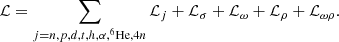 (1)
(1)
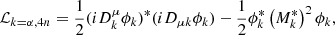
The couplings of the clusters to the mesons are defined in terms of the couplings of the nucleons, gs, gv, gρ to the σ-, ω-, and ρ-mesons, respectively. For the fermionic clusters, j = t, h, we have
![Mathematical equation: $$ \begin{aligned} \mathcal{L}_j = \bar{\psi }\left[\gamma _\mu i D_j^\mu - M_j^*\right]\psi , \end{aligned} $$](/articles/aa/full_html/2023/11/aa47496-23/aa47496-23-eq2.gif) (2)
(2)
with
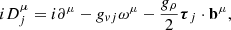 (3)
(3)
where τj are the Pauli matrices and gvj is the coupling of cluster j to the vector meson ω, which is defined as gvj = Ajgv for all clusters.
The Lagrangian density for the bosonic clusters, j = d, α,6He, and 4n, is given by
 (4)
(4)
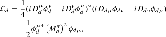 (5)
(5)
with
 (6)
(6)
For the nucleonic gas, j = n, p, we have
![Mathematical equation: $$ \begin{aligned} \mathcal{L}_j = \bar{\psi }\left[\gamma _\mu i D^\mu - m^*\right]\psi ,\end{aligned} $$](/articles/aa/full_html/2023/11/aa47496-23/aa47496-23-eq7.gif) (7)
(7)
with
 (8)
(8)
 (9)
(9)
For the fields, we have the standard RMF expressions:
 (10)
(10)
where Ωμν = ∂μVν − ∂νVμ and Bμν = ∂μbν − ∂νbμ − gρ(bμ × bν).
The total binding energy of a light cluster j is given by
 (11)
(11)
with  the effective mass of cluster j, which is determined by the meson coupling as well as by a binding energy shift:
 (12)
(12)
In expression (12),  is the binding energy of the cluster j = 2H, 3H, 3He, 4He,6He in the vacuum, and these constants are fixed to experimental values. For the tetraneutron, we take the values of Duer et al. (2022). We take the binding energy of the tetraneutron,
  , as negative, as it is considered a resonant state in Duer et al. (2022), while the other five light clusters, being bound states, have positive binding energies.
The binding energy shift δBj is given by (Pais et al. 2018)
 (13)
(13)
This term acts as the energetic counterpart of the excluded volume mechanism in the Thomas-Fermi approximation. ρ0 is the nuclear saturation density, Nj and Zj are the neutron and proton numbers, and  and
and  are the energy density and density of the lowest energy levels of the gas, respectively. This means that the energy states occupied by the gas are removed from the calculation of the cluster binding energy, which circumvents double-counting of the particles of gas and those of the clusters.
Regarding the scalar and vector cluster–meson couplings, we follow the prescription introduced in Pais et al. (2018). The scalar coupling is given by
 (14)
(14)
while the vector coupling is given by
 (15)
(15)
Here, Aj corresponds to the number of nucleons in cluster j. The xs factor can vary from 0 to 1. In a previous work, its value was fixed to xs = 0.85 ± 0.05 from a fit to the Virial EoS. In later works, the value was found to be higher, xs = 0.92 ± 0.02, when a fit to experimental data was considered (Pais et al. 2020a,b). In the following, we use both couplings to test its effect on the clusters abundances. The dissolution of the clusters is affected by a combination of both the binding energy shift, δBj, and this factor xs. Substituting Eqs. (12), (9), and (14) into Eq. (11), we obtain
 (16)
(16)
For the two extreme cases, we have
 (17)
(17)
 (18)
(18)
This implies that a larger xsj corresponds to a larger binding energy, and consequently the dissolution of the cluster occurs at larger densities. If xsj = 1, the dissolution is totally defined by the binding shift δBj. We note that at finite temperature, the clusters dissolve at a density well above that for which Bj ∼ 0. For this reason, the tetraneutron survives even as a resonance. The larger the temperature, the more the fraction of clusters is defined by their mass and isospin, and not by the binding energy.
With the same set of couplings determined in the previous section, we calculate the chemical equilibrium constants:
![Mathematical equation: $$ \begin{aligned} K_{\rm c}[j]=\frac{\rho _j}{\rho _{\rm n}^{N_j}\rho _{\rm p}^{Z_j}} ,\end{aligned} $$](/articles/aa/full_html/2023/11/aa47496-23/aa47496-23-eq24.gif) (19)
(19)
where ρj is the number density of cluster j, and ρp and ρn are the number densities of free protons and neutrons, respectively.
Even though there are no experimental Kc for the tetraneutron, we calculate it for the other clusters, considering calculations where we do and do not include the 4n. This may provide clues as to the abundance of the clusters, and the presence or not of the tetraneutron.
Let us also refer to another point that must be discussed. The tetraneutron, as in the other light clusters in this work, is treated as a point-like particle, and one may ask whether or not an exclusion volume should be included in order that the model does not break down as the temperature increases. In this model, the role of the exclusion volume – included, for instance, in Lattimer & Swesty (1991) or in Shen et al. (1998) – is undertaken by the ω-meson, as clearly discussed in Typel et al. (2010) and Avancini et al. (2010). We do not therefore consider any explicit exclusion volume term.
3. Results
In this section, we show the mass fractions of the clusters and discuss how they are affected by temperature and isospin asymmetry of the medium. We define them as
 (20)
(20)
In particular, we discuss how the fraction of the classical clusters are affected by the presence of the tetraneutron. For the couplings xsj, we take the values 0.85 and 0.92 as determined in Pais et al. (2018) and Pais et al. (2020a), respectively, fitting our model to two different sets of experimental data (Qin et al. 2012; Bougault et al. 2020). The value xsj = 0.85 was found from a fit to the Virial EoS (Pais et al. 2018). Later, when fitting other experimental data from the INDRA collaboration, we found that the calibration would need a larger coupling, which means larger binding energies, and therefore a larger dissolution density. This value was found to be xsj = 0.92 (Pais et al. 2020a).
3.1. The energy of the tetraneutron
Here we show the different abundances obtained when considering different energies for the tetraneutron.
We consider its energy to be given by two bands, with the following extremes:
![Mathematical equation: $$ \begin{aligned}&B^0_{4n}= -2.37 \pm \sqrt{0.38^2 + 0.44^2} = [-2.95:-1.79], \end{aligned} $$](/articles/aa/full_html/2023/11/aa47496-23/aa47496-23-eq26.gif) (21)
(21)
![Mathematical equation: $$ \begin{aligned}&B^0_{4n}= -2.37 \pm 1.8\Gamma = [-5.52:0.78], \end{aligned} $$](/articles/aa/full_html/2023/11/aa47496-23/aa47496-23-eq27.gif) (22)
(22)
both defined in MeV. The width Γ is equal to 1.75 MeV. Equation (21) considers both the systematic and statistical errors in the energy value, and does not take into account the width of the resonance, whereas Eq. (22) considers Γ, multiplied by a factor, obtained if the width distribution is Cauchy-type. The derivation of this factor is given in Appendix A. We note that the tetraneutron properties are yet uncertain and have varied from previous calculations (Ivanytskyi et al. 2019).
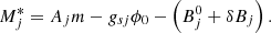
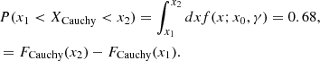
Taking these binding energies and uncertainties, we calculate and discuss how the 4n and light cluster abundances vary with density. In Fig. 1, the mass fractions of the clusters d, t, h, α, 6He, and 4n are plotted for a proton fraction typical of a NS, yp = 0.1, and two representative temperatures, 4 and 10 MeV. We also consider two values of the coupling of the clusters to the σ-meson, as explained above. In Fig. 1, for the 4n, we take the binding energy defined by the range given in Eq. (21), which is shown by the solid bands. The crossed bands are obtained by taking the range defined by Eq. (22) instead. These define slightly wider regions, but the same overall behavior is obtained.
 |
Fig. 1. Mass fractions as a function of density when considering different energy bands for the tetraneutron, for T = 4 (left) and 10 (right) MeV, and two different scalar couplings for the clusters, xs = 0.92 (top) and xs = 0.85 (bottom). |
For this small proton fraction, it is striking that at the maximum of the clusters, the mass fraction of the 4n cluster is the largest among the clusters and can be as large as that of free neutrons if xsj = 0.92, and just slightly smaller for xsj = 0.85. On the other hand, 4n is the first cluster to dissolve. At T = 10 MeV, the 4n is still the most abundant cluster but the impact on the free nucleons is not as strong as for T = 4 MeV. For a temperature of 10 MeV, it is the neutron content and the magnitude of the mass that define the cluster abundances (and not the binding energy): 4n are still the most abundant at ρ ∼ 0.02 fm−3 due to the neutron content, followed by the t and the d; the former because it is the next cluster in mass with the largest neutron content and the latter because it is the lightest cluster.
We see that the abundance of the tetraneutron increases for the low-T and high-xsj case. We also observe that by even considering two different ranges for the energy of the 4n, the difference in the abundances of the other clusters is not significant. This difference is only non-negligible at the maximum of the 4n abundance; that is, both at the onset and dissolution, the difference is completely negligible.
This implies that such a binding energy of the tetraneutron will not make a significant difference in the systems considered, that is, in conditions typical of core-collapse supernovae or heavy-ion collisions, where these clusters are also measured. The impact of 4n clusters would be higher in more neutron-rich systems.
In order to better quantify the effect of the inclusion of the 4n clusters, in the following section we concentrate our discussion on the ratios of quantities calculated with and without the tetraneutron.
3.2. Effect of including 4n
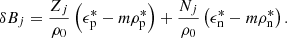
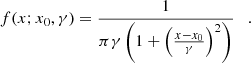
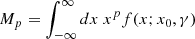
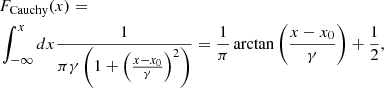
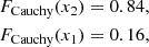
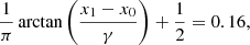
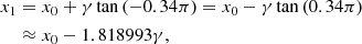
In this subsection, we compare the effect of including 4n in the matter by defining particle fractions and equilibrium constant ratios between the quantities obtained with and without the inclusion of 4n particles. In Figs. 2–4, we plot the ratio of the mass fractions of the five light clusters and of the gas, and of the chemical equilibrium constants of the five light clusters, in a calculation with and without the tetraneutron against the baryonic density, using the FSU model, fixed temperatures of 4, 10, and 20 MeV, and two proton fractions, yp = 0.1, and 0.3. The scalar cluster–meson coupling is chosen as xsj = 0.85 and 0.92. The energy of the tetraneutron is chosen as  MeV, which is the average value of Duer et al. (2022), taken as a negative value in order to consider it as a resonant state, as opposed to a bound state as in the other clusters considered, whose binding energy value in the vacuum is taken to be positive. We observe that all clusters dissolve below 0.1 fm−3, including the tetraneutron. The fraction maxima move from ∼0.01 fm−3 at T = 4 MeV to ∼0.05 fm−3 for T = 20 MeV.
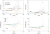 |
Fig. 2. Ratio of the mass fractions of the clusters and of the gas (top panels) with (Yi(w)) and without (Yi(wo)) the tetraneutron, for a fixed proton fraction of yp = 0.3 (left) and yp = 0.1 (right), in a calculation where we consider a fixed binding energy for the 4n, taken as B0(4n) = − 2.37 MeV. In the bottom panels, the chemical equilibrium constants, Kc[i], in a calculation with (w) and without (wo) the tetraneutron, are shown in the same conditions as the top panels. In all panels, the temperature is fixed to 4 MeV, the FSU EoS is considered, and the scalar cluster–meson coupling is taken as xs = 0.85 (solid) and xs = 0.92 (dashed). |
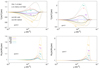 |
Fig. 3. Ratio of the mass fractions of the clusters and of the gas (top panels) with (Yi(w)) and without (Yi(wo)) the tetraneutron, for a fixed proton fraction of yp = 0.3 (left), and yp = 0.1 (right), in a calculation where we consider a fixed binding energy for the 4n, taken as B0(4n) = − 2.37 MeV. In the bottom panels, the chemical equilibrium constants, Kc[i], in a calculation with (w) and without (wo) the tetraneutron, are shown in the same conditions as the top panels. In all panels, the temperature is fixed to 10 MeV, the FSU EoS is considered, and the scalar cluster–meson coupling is taken as xs = 0.85 (solid) and xs = 0.92 (dashed). We highlight the different y-axis scales. |
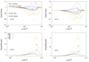 |
Fig. 4. Ratio of the mass fractions of the clusters and of the gas (top panels) with (Yi(w)) and without (Yi(wo)) the tetraneutron, for a fixed proton fraction of yp = 0.3 (left), and yp = 0.1 (right), in a calculation where we consider a fixed binding energy for the 4n, taken as B0(4n) = − 2.37 MeV. In the bottom panels, the chemical equilibrium constants, Kc[i], in a calculation with (w) and without (wo) the tetraneutron, are shown in the same conditions as the top panels. In all panels, the temperature is fixed to 20 MeV, the FSU EoS is considered, and the scalar cluster–meson coupling is taken as xs = 0.85 (solid) and xs = 0.92 (dashed). |
The role of the scalar cluster–meson coupling in the abundances of the clusters should also be discussed. Considering both values allows us to see how this coupling affects the mass fractions and to estimate the uncertainty connected to the calibration of the underlying model used to perform the calculations.
For the lowest temperature considered, shown in Fig. 2, we observe that the proton-rich and symmetric clusters, such as 3He or 4He, increase in abundance, whereas the abundance of neutron-rich cluster decreases, as the neutrons are being consumed by the tetraneutron. The effect is greater for the low-temperature and low-proton fraction system. When we increase the temperature (see Figs. 3 and 4), we see that the abundance of the proton-rich clusters decreases, and looking for example at the α-particle, for yp = 0.1, there is only a tiny range in density where it becomes more abundant when 4n is included. Looking at 3He, this never happens: its abundance is always higher in the calculation with 4n, that is, in all the temperatures and proton fractions considered. We also observe that the higher the scalar coupling, the higher the abundance, simultaneously shifting the dissolution density of the clusters to larger values.
The bottom panels of these figures show the ratio of the chemical equilibrium constants with and without 4n. For T = 10 and 20 MeV, the neutron-rich clusters, such as 6He, show an increase when the tetraneutron is included in the calculation, in the high-density limit. For the lowest temperature considered, this is also seen, though to a lesser extent, with the effect being more prominent in the low-proton fraction case.
We now look in more detail at the mass fractions of the proton and neutron background gas and of the 4He fractions, particles that have a special role in the transport coefficients (the first two) or in the dissolution of the accretion disk of a neutron star binary merger (Rosswog 2015). In order to allow for a clearer discussion, these are represented in Fig. 5, where they are compared for the three temperatures considered in the present study (4, 10, and 20 MeV) and for the two proton fractions (0.3 and 0.1). Some conclusions can be made here: (i) the effect of the inclusion of the 4n is higher in the low-temperature and low-proton fraction case, as already discussed above; (ii) in a rich neutron environment, the effect is quite dramatic, with a possible increase in the proton fraction of more than 500% and an increase in the α-particle fraction of ∼300% if T = 4 MeV and xsj = 0.92 are considered (we note that we are plotting the ratios divided by three in this panel). Even for T = 10 MeV, the increase in the proton fraction is about 100% and that in the α fraction is ∼33%; and (iii) the neutron fraction is directly affected, suffering a notable reduction, although not as strong a reduction as the proton fraction. It is observed that the reduction is ≲0.5 and does not vary significantly with temperature.
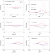 |
Fig. 5. Ratio of the mass fractions of the proton and neutron gas and of the α particles with (Yi(w)) and without (Yi(wo)) the tetraneutron for a fixed proton fraction of yp = 0.3 (left) and yp = 0.1 (right) and T = 4 (top), 10 (middle) and 20 (bottom) MeV, in a calculation where we take the binding energy of the 4n as −2.37 MeV. In all panels, the FSU EoS is considered, and the scalar cluster–meson coupling is taken as xs = 0.85 (solid) and xs = 0.92 (dashed). We highlight the fact that the scale of the y-axis of the bottom panels is different, and the ratio of the top right panel is divided by 3. |
3.3. The chemical equilibrium constants
As these clusters are also observed in heavy-ion collisions, we plot the ratio of the chemical equilibrium constants of the clusters in a calculation with and without the tetraneutron in the top panel of Fig. 6, considering T = 5 MeV and a proton fraction of 0.41, which is the value found in the Texas experiment (Qin et al. 2012), and the scalar cluster–meson coupling fixed to 0.85. We considered one of the temperatures measured that is more sensitive to the presence of tetraneutrons. As discussed above, we see that the difference in the chemical equilibrium constants with and without 4n is not large, except for the high-density limit where we see that the most neutron-rich cluster increases. We note that the experimental data were measured for a relatively symmetric system, yp = 0.41, and the tetraneutron plays an important role in very asymmetric matter.
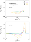 |
Fig. 6. Ratio between the chemical equilibrium constants with and without the tetraneutron, Kc[i], as a function of density. In the calculation with 4n, we take its binding energy as |

In the bottom panel, we use xsj = 0.92 for the scalar cluster–meson coupling, as determined by Pais et al. (2020a). As discussed above, the effect of the tetraneutron inclusion is stronger and this is reflected in the chemical equilibrium ratio, which increases for a larger coupling.
4. Conclusions
We analyzed the effects of the presence of the 4n cluster in hot matter formed in astrophysical environments such as binary NS mergers or core-collapse supernova matter. In particular, we thoroughly discuss how their presence affects the abundances of the other light clusters.
This discussion was undertaken within the framework of the RMF description of inhomogeneous matter calibrated to nuclear matter properties (Pais et al. 2018) and the formation of light clusters in heavy-ion collisions (Qin et al. 2012; Pais et al. 2020a). This framework allows the inclusion of light clusters as new degrees of freedom, and the couplings of the cluster fields to the mesons inherent to the model allow us to modulate the effects of the medium; in particular, their dissolution.
We show that the presence of 4n increases the abundances of free protons and α particles while decreasing the abundance of free neutrons. The effects are stronger in very neutron-rich matter and for lower temperatures. For T = 5 MeV, the abundance of free protons could increase by a factor of 5 at the peak of the cluster fractions that occurs at ∼0.02 fm−3, which would therefore have an effect on transport properties, such as conductivity. Also, an increase in the α fractions may affect the evolution of the dissolution of the disk formed in a NS merger, as discussed by Rosswog (2015). Presently, HICs occur for relatively symmetric systems and therefore the presence of 4n will be difficult to detect. In the best conditions, that is, with the lowest temperature detected, we did not find an effect of greater than 2%, which is certainly difficult to detect.
Acknowledgments
H.P. thanks J. Natowitz and G. Röpke for useful discussions and for bringing to her attention the work of Duer et al. (2022). H.P. and C.P. acknowledge the FCT (Portugal) Projects No. 2021.09262.CBM, 2022.06460.PTDC, UIDB/FIS/04564/2020, and UIDP/FIS/04564/2020. C.A. and M.A.P.G. acknowledge the support of the Agencia Estatal de Investigación through the grants PID2019-107778GB-100, PID2022-137887NB-I00, and from Junta de Castilla y León, SA096P20 project.
References
- Andronic, A., Braun-Munzinger, P., & Stachel, J. 2006, Nucl. Phys. A, 772, 167 [NASA ADS] [CrossRef] [Google Scholar]
- Arcones, A., Martínez-Pinedo, G., O’Connor, E., et al. 2008, Phys. Rev. C, 78, 015806 [NASA ADS] [CrossRef] [Google Scholar]
- Avancini, S. S., Barros, C. C., Jr, Menezes, D. P., & Providência, C. 2010, Phys. Rev. C, 82, 025808 [NASA ADS] [CrossRef] [Google Scholar]
- Avancini, S. S., Ferreira, M., Pais, H., Providência, C., & Röpke, G. 2017, Phys. Rev. C, 95, 045804 [NASA ADS] [CrossRef] [Google Scholar]
- Bauswein, A., Goriely, S., & Janka, H.-T. 2013, ApJ, 773, 78 [NASA ADS] [CrossRef] [Google Scholar]
- Bougault, R., Bonnet, E., Borderie, B., et al. 2020, J. Phys. G, 47, 025103 [NASA ADS] [CrossRef] [Google Scholar]
- Cauchy Distribution 2008, in the Concise Encyclopedia of Statistics (New York: Springer) [Google Scholar]
- Duer, M., Aumann, T., & Gernhäuser, R. 2022, Nature, 606, 678 [NASA ADS] [CrossRef] [Google Scholar]
- Ferreira, M., & Providência, C. 2012, Phys. Rev. C, 85, 055811 [NASA ADS] [CrossRef] [Google Scholar]
- Hempel, M., & Schaffner-Bielich, J. 2010, Nucl. Phys. A, 837, 210 [Google Scholar]
- Horowitz, C. J., & Schwenk, A. 2006a, Phys. Lett. B, 638, 153 [CrossRef] [Google Scholar]
- Horowitz, C. J., & Schwenk, A. 2006b, Nucl. Phys. A, 776, 55 [CrossRef] [Google Scholar]
- Ivanytskyi, O., Pérez-García, M. A., & Albertus, C. 2019, Eur. Phys. J. A, 55, 184 [NASA ADS] [CrossRef] [Google Scholar]
- Kisamori, K., Shimoura, S., Miya, H., et al. 2016, Phys. Rev. Lett., 116, 052501 [NASA ADS] [CrossRef] [Google Scholar]
- Lattimer, J. M., & Swesty, D. F. 1991, Nucl. Phys. A, 535, 331 [CrossRef] [Google Scholar]
- Marqués, F. M., Labiche, M., Orr, N. A., et al. 2002, Phys. Rev. C, 65, 044006 [CrossRef] [Google Scholar]
- Marqués, F. M., Orr, N. A., Al Falou, H., et al. 2005, arXiv e-prints [arXiv:nucl-ex/0504009] [Google Scholar]
- Oertel, M., Hempel, M., Klähn, T., & Typel, S. 2017, Rev. Mod. Phys., 89, 015007 [Google Scholar]
- Pais, H., Chiacchiera, S., & Providência, C. 2015, Phys. Rev. C, 91, 055801 [NASA ADS] [CrossRef] [Google Scholar]
- Pais, H., Gulminelli, F., Providência, C., & Röpke, G. 2018, Phys. Rev. C, 97, 045805 [NASA ADS] [CrossRef] [Google Scholar]
- Pais, H., Gulminelli, F., Providência, C., & Röpke, G. 2019, Phys. Rev C, 99, 055806 [NASA ADS] [CrossRef] [Google Scholar]
- Pais, H., Bougault, R., Gulminelli, F., et al. 2020a, Phys. Rev. Lett., 125, 012701 [CrossRef] [Google Scholar]
- Pais, H., Bougault, R., Gulminelli, F., et al. 2020b, J. Phys G., 47, 105204 [NASA ADS] [CrossRef] [Google Scholar]
- Pérez García, M. A., Izzo, L., Barba-González, D., et al. 2022, A&A, 666, A67 [CrossRef] [EDP Sciences] [Google Scholar]
- Prada, F., Content, R., Goobar, A., et al. 2020, ArXiv e-prints [arXiv:2007.01603] [Google Scholar]
- Qin, L., Hagel, K., Wada, R., et al. 2012, Phys. Rev. Lett., 108, 172701 [CrossRef] [Google Scholar]
- Raduta, Ad. R., & Gulminelli, F. 2010, Phys. Rev. C, 82, 065801 [NASA ADS] [CrossRef] [Google Scholar]
- Raduta, Ad. R., & Gulminelli, F. 2019, Nucl. Phys. A, 983, 252 [NASA ADS] [CrossRef] [Google Scholar]
- Röpke, G. 2015, Phys. Rev. C, 92, 054001 [CrossRef] [Google Scholar]
- Rosswog, S. 2015, Int. J. Mod. Phys. D, 24, 1530012 [NASA ADS] [CrossRef] [Google Scholar]
- Shen, H., Toki, H., Oyamatsu, K., & Sumiyoshi, K. 1998, Nucl. Phys. A, 637, 435 [Google Scholar]
- Todd-Rutel, B. G., & Piekarewicz, J. 2005, Phys. Rev. Lett., 95, 122501 [NASA ADS] [CrossRef] [Google Scholar]
- Typel, S., Röpke, G., Klähn, T., Blaschke, D., & Wolter, H. H. 2010, Phys. Rev. C, 81, 015803 [NASA ADS] [CrossRef] [Google Scholar]
- Voskresenskaya, M. D., & Typel, S. 2012, Nucl. Phys. A, 887, 42 [NASA ADS] [CrossRef] [Google Scholar]
- Wu, X.-H., Wang, S.-B., Sedrakian, A., & Röpke, G. 2017, J. Low Temp. Phys., 189, 133 [NASA ADS] [CrossRef] [Google Scholar]
Appendix A: The Cauchy distribution
The Cauchy (or Lorentz, or Breit-Wigner) probability density is defined as (see e.g., Ivanytskyi et al. (2019), Andronic et al. (2006), Cauchy Distr. (2008))
 (A.1)
(A.1)
All the moments of this distribution are undefined, because
 (A.2)
(A.2)
diverges. In particular, expected value, variance, and curtosis are undefined. This distribution is symmetric and its median is x0, which is the central value. The x0 − γ and x0 + γ points are the first and third quartiles, respectively.
The distribution function of the Cauchy probability density is
 (A.3)
(A.3)
which is the integrated probability that the random variable XCauchy satisfies XCauchy < x
In the normal distribution, the variance σ of the distribution, which is identified with the uncertainty, satisfies the condition that
 (A.4)
(A.4)
where x0 is the mean or expected value of the normal distribution.
As we are dealing with a distribution of mass under the Cauchy law, in order to establish an analogy with the normal distribution, we propose to identify the median with the mean. To build an error interval with a 68% probability, as in the normal distribution, we need to calculate the two points, such that
 (A.5)
(A.5)
As the probability density is symmetric
 (A.6)
(A.6)
and x1, 2 will satisfy
 (A.7)
(A.7)
Therefore, as
 (A.8)
(A.8)
then, straightforwardly,
 (A.9)
(A.9)
and subsequently,
 (A.10)
All Figures
|
Fig. 1. Mass fractions as a function of density when considering different energy bands for the tetraneutron, for T = 4 (left) and 10 (right) MeV, and two different scalar couplings for the clusters, xs = 0.92 (top) and xs = 0.85 (bottom). |
| In the text | |
|
Fig. 2. Ratio of the mass fractions of the clusters and of the gas (top panels) with (Yi(w)) and without (Yi(wo)) the tetraneutron, for a fixed proton fraction of yp = 0.3 (left) and yp = 0.1 (right), in a calculation where we consider a fixed binding energy for the 4n, taken as B0(4n) = − 2.37 MeV. In the bottom panels, the chemical equilibrium constants, Kc[i], in a calculation with (w) and without (wo) the tetraneutron, are shown in the same conditions as the top panels. In all panels, the temperature is fixed to 4 MeV, the FSU EoS is considered, and the scalar cluster–meson coupling is taken as xs = 0.85 (solid) and xs = 0.92 (dashed). |
| In the text | |
|
Fig. 3. Ratio of the mass fractions of the clusters and of the gas (top panels) with (Yi(w)) and without (Yi(wo)) the tetraneutron, for a fixed proton fraction of yp = 0.3 (left), and yp = 0.1 (right), in a calculation where we consider a fixed binding energy for the 4n, taken as B0(4n) = − 2.37 MeV. In the bottom panels, the chemical equilibrium constants, Kc[i], in a calculation with (w) and without (wo) the tetraneutron, are shown in the same conditions as the top panels. In all panels, the temperature is fixed to 10 MeV, the FSU EoS is considered, and the scalar cluster–meson coupling is taken as xs = 0.85 (solid) and xs = 0.92 (dashed). We highlight the different y-axis scales. |
| In the text | |
|
Fig. 4. Ratio of the mass fractions of the clusters and of the gas (top panels) with (Yi(w)) and without (Yi(wo)) the tetraneutron, for a fixed proton fraction of yp = 0.3 (left), and yp = 0.1 (right), in a calculation where we consider a fixed binding energy for the 4n, taken as B0(4n) = − 2.37 MeV. In the bottom panels, the chemical equilibrium constants, Kc[i], in a calculation with (w) and without (wo) the tetraneutron, are shown in the same conditions as the top panels. In all panels, the temperature is fixed to 20 MeV, the FSU EoS is considered, and the scalar cluster–meson coupling is taken as xs = 0.85 (solid) and xs = 0.92 (dashed). |
| In the text | |
|
Fig. 5. Ratio of the mass fractions of the proton and neutron gas and of the α particles with (Yi(w)) and without (Yi(wo)) the tetraneutron for a fixed proton fraction of yp = 0.3 (left) and yp = 0.1 (right) and T = 4 (top), 10 (middle) and 20 (bottom) MeV, in a calculation where we take the binding energy of the 4n as −2.37 MeV. In all panels, the FSU EoS is considered, and the scalar cluster–meson coupling is taken as xs = 0.85 (solid) and xs = 0.92 (dashed). We highlight the fact that the scale of the y-axis of the bottom panels is different, and the ratio of the top right panel is divided by 3. |
| In the text | |
|
Fig. 6. Ratio between the chemical equilibrium constants with and without the tetraneutron, Kc[i], as a function of density. In the calculation with 4n, we take its binding energy as |
| In the text | |
Current usage metrics show cumulative count of Article Views (full-text article views including HTML views, PDF and ePub downloads, according to the available data) and Abstracts Views on Vision4Press platform.
Data correspond to usage on the plateform after 2015. The current usage metrics is available 48-96 hours after online publication and is updated daily on week days.
Initial download of the metrics may take a while.