| Issue |
A&A
Volume 679, November 2023
|
|
|---|---|---|
| Article Number | A8 | |
| Number of page(s) | 9 | |
| Section | Stellar atmospheres | |
| DOI | https://doi.org/10.1051/0004-6361/202243458 | |
| Published online | 31 October 2023 | |
The inner dust shell of Betelgeuse seen with high-angular-resolution polarimetry★
1
European Organisation for Astronomical Research in the Southern Hemisphere,
Casilla
19001,
Santiago 19,
Chile
e-mail: xhaubois@eso.org
2
Univ. Grenoble Alpes, CNRS, IPAG,
38000
Grenoble, France
3
School of Physics and Astronomy, Monash University,
Clayton, VIC
3800, Australia
4
IRAP, Université de Toulouse, CNRS, CNES,
UPS. 14, Av. E. Belin.
31400
Toulouse, France
5
IRAP, Université de Toulouse, CNRS, UPS, CNES,
57 avenue d’Azereix,
65000
Tarbes, France
6
LESIA, Observatoire de Paris, Université PSL, CNRS, Sorbonne Université, Université de Paris,
5 place Jules Janssen,
92195
Meudon, France
Received:
3
March
2022
Accepted:
9
August
2023
Context. The characteristics of the innermost layer of dust winds from red supergiants have not been identified. In 2019–2020, Betelgeuse exhibited an important dimming event that has been partially attributed to dust formation, highlighting the importance of understanding dust properties in the first stellar radii from the photosphere.
Aims. We aim to detect and characterize the inner dust environment of Betelgeuse at high spatial resolution.
Methods. We obtained SPHERE/ZIMPOL and SPHERE/IRDIS linear polarimetric observations from January 2019, before the dimming event, and compared them to a grid of synthetic radiative transfer models.
Results. We detect a structure that is relatively centro-symmetric with a 60 mas diameter (1.3–1.4 stellar diameter). We computed synthetic images using radiative transfer modeling assuming a spherical dust shell composed of MgSiO3 grains. We find that most of the data are best reproduced with a dust shell whose outer radius is approximately 10 AU (i.e., ~2 stellar radii) and a maximum grain size in the 0.4–0.6 µm range. These results are close to the ones we obtained from 2013 NACO/SAMPOL data, indicating that the shell radius and grain size can show some stability for at least 6 yr despite morphological changes of the dust shell. The residuals after the subtraction of the best-fitting centro-symmetric model suggest complex asymmetric density structures and photospheric effects.
Key words: techniques: high angular resolution / supergiants / infrared: stars / stars: individual: Betelgeuse
© The Authors 2023
 Open Access article, published by EDP Sciences, under the terms of the Creative Commons Attribution License (https://creativecommons.org/licenses/by/4.0), which permits unrestricted use, distribution, and reproduction in any medium, provided the original work is properly cited.
This article is published in open access under the Subscribe to Open model. Subscribe to A&A to support open access publication.
1 Introduction
Dust is a vector and product of the mass-loss phenomenon at play in red supergiants (RSGs). This mechanism has an important role in the evolution of RSGs into type-II supernovae as well as in galactic chemical enrichment. The formation loci and properties of the first stage of a dust wind have not been established. Evidence for dust has been reported around the emblematic M2 type RSG Betelgeuse (α Orionis, HD39801) in its very close environment. Reconstructed images from speckle interferometry show an asymmetric structure at ~2–2.5 stellar radii (Roddier & Roddier 1985). More recent mid-infrared observations revealed a complex dust environment (Kervella et al. 2011) compatible with a silicate or alumina composition, confirming previous interferometric diagnostics from Verhoelst et al. (2006) and Perrin et al. (2007).
In December 2019, Betelgeuse underwent a dimming event that has been reported and analysed in various papers (e.g., Dupree et al. 2020; Montargès et al. 2021; Kravchenko et al. 2021; Taniguchi et al. 2022). However, it is not clear if this event can be entirely attributed to dust formation (Harper et al. 2020), and this has emphasized the importance of understanding the conditions for dust formation when interpreting variability from RSGs.
Polarimetry at high angular resolution is a powerful technique for investigating circumstellar dust environments. In Haubois et al. (2019, hereafter H2019), we modeled a structure detected in linearly polarized light as a thin dust shell located only 0.5 stellar radii above Betelgeuse’s photosphere (corresponding to a dust shell radius of about 7.3 AU with a distance of 222 pc; Harper et al. 2017) from sparse aperture-masking polarimetric interferometry data (NACO/SAMPOL). This so-called inner dust shell (IDS) poses interesting constraints on the survival of dust grains. At that short distance from the photosphere, the local temperature can reach the 1500–2000 K range, implying dust material with high condensation and sublimation temperatures. From comparisons with SPHERE/ZIMPOL measurements, we show in H2019 that radiative transfer models favor a dust composition made of MgSiO3 (enstatite) and Mg2SiO4 (forsterite) over Al2O3 (alumina). In an attempt to elaborate on the findings presented in H2019, we report here on SPHERE/ZIMPOL and SPHERE/IRDIS kinear polarimetric observations obtained January 18–19, 2019. After presenting the observations and their analysis in Sects. 2 and 3, respectively, we compare the images of polarized intensity with radiative transfer models in Sect. 4. Subsequently, we present the discussion and conclusions in Sects. 5 and 6, respectively.
2 Observations
We observed Betelgeuse on January 17 and 18, 2019, with SPHERE (Beuzit et al. 2019) at the Very Large Telescope at visible wavelengths with ZIMPOL (Schmid et al. 2018) and at near-infrared wavelengths with IRDIS (Dohlen et al. 2008; de Boer et al. 2020; van Holstein et al. 2020). Data were taken in linear polarimetric modes in ten filters, including those of a point spread function (PSF) calibrator star, Phi2 Orionis. The total intensity images are presented in Fig. 1, and Table 1 summarizes the observations. Atmospheric conditions were good and stable throughout the Betelgeuse and calibrator observations. However, we experienced a low-wind effect (Milli et al. 2018). This had the impact of decreasing the Strehl ratio (SR) as measured from the SPHERE images compared to the SPARTA SR measurements. The ZIMPOL and IRDIS data were reduced by the SPHERE Data Center (Delorme et al. 2017) and using the IRDAP1 pipeline (van Holstein et al. 2017, 2020), respectively. For ZIMPOL data, we estimated the instrumental polarization to be less than 0.1% for all filters by computing it over the halo of starlight in the images, a result consistent with the findings from Schmid et al. (2018). With IRDAP, we subtracted the instrumental polarization using the Mueller matrix model and then subtracted the stellar polarization from the halo of starlight. We followed the IRDAP convention in terms of orientation of polarization direction. From the Q and U images, we then computed images of the azimuthal Stokes parameters Qϕ and Uϕ following the definitions of de Boer et al. (2020) as well as images of the linearly polarized intensity,  . The images of the Stokes parameters Q and U reveal “butterfly patterns” in all filters (see Fig. 2), as expected for centro-symmetric polarization created from scattering off a face-on structure such as a disk or a sphere.
In order to remove instrumental polarization (IP) effects, it is possible to use techniques such as minimizing the azimuthal Stokes parameter, Uϕ. (Avenhaus et al. 2014; de Boer et al. 2020). Because there should be no radial polarization, we applied a minimization technique to the negative Qϕ signal in order to remove residual IP in our ZIMPOL data set. Due to the better spatial resolution delivered by ZIMPOL, there were enough pixels in the images to efficiently remove spurious polarization. This was not possible in the case of the IRDIS data set. We therefore used the Uϕ minimization technique in that case as the IP-generated butterfly pattern clearly dominated in these images.
In the V-band filter, we observed that the butterfly pattern had a different orientation from all the other filters. The reason for this could in principle be astrophysical as, for thick dusty stellar environments such as protoplanetary disks, multiple scattering can lead to non-azimuthal linear polarization effects (azimuthal Stokes Uϕ signal is non-null; see Canovas et al. 2015). However, in our case, the angle of linear polarization (AoLP) is azimuthal at all the other wavelengths from the visible to the near-infrared, so it is more likely that the cause for this V-band-specific polarization effect is of instrumental origin. Having corrected for instrumental polarization, we suggest that this issue originates from a so-far uncharacterized instrumental crosstalk.
The polarimetric design of ZIMPOL (Schmid et al. 2018) includes two half-wave plates (HWP2 and HWPZ) that together prevent the creation of instrumental crosstalk by SPHERE’s image derotator (K-mirror) when the derotator moves in field-tracking (P2) mode. HWP2 rotates the polarization directions to be measured by ZIMPOL such that they are parallel and perpendicular to the plane of reflection of the derotator. As a result, the derotator does not create instrumental crosstalk. HWPZ, located within ZIMPOL, then rotates the to-be-measured polarization directions back to their original orientation. However, before the light reaches HWPZ, it is reflected off several silver-coated mirrors. Because the polarization directions are now not aligned parallel or perpendicular to the planes of reflection of these mirrors, these mirrors could create crosstalk, predominantly at short wavelengths. To validate this scenario, it is necessary to measure Mueller matrices in the V band and in other filters for comparison. This instrumental task is still pending.
To correct the orientation of the butterfly pattern of the Q and U images in the V band, we referred to procedures outlined in Appendix C of Avenhaus et al. (2014) and in de Boer et al. (2020) for the case of the correction of instrumental polarization. We first set the AoLP to be azimuthally oriented. We did this by finding the angular offset for the linear polarization that minimizes the sum of the squared signal in the image of the azimuthal Stokes parameter, Uϕ. After fitting the offset, we converted the images back to Q and U, and the butterfly patterns then presented a similar orientation as in the other filters. In practice, we performed this step in the same iteration loop as the Qϕ minimization designed to remove residual instrumental polarization as described above. The comparison between the data before and after the Uϕ and Qϕ minimizations is presented in Fig. 2. However, even though the orientation of the butterfly pattern was corrected by this technique, the polarized intensity cannot be fully retrieved as we do not know the amount of polarization signal that is lost due to the crosstalk. A modeling of this instrumental loss remains beyond the scope of the present work. We therefore disregard V-band filter data in the rest of the paper.
For the ZIMPOL observations, the PSF reference star Phi2 Ori (stellar parameters from Bordé et al. 2002, and references therein) could not be used to calibrate the photometry of our images as atmospheric transparency conditions were too unstable (the so-called THICK category, transparency variations above 20%) between Betelgeuse and this calibrator (see Fig. 3). However, the IRDIS data points (wavelengths above 1 µm) were taken the night before, when the atmosphere was more transparent (so-called CLEAR conditions). Those near-infrared Betelgeuse measurements were calibrated with Phi2 Ori measurements and fitted by an ATLAS9 stellar atmosphere model (Castelli & Kurucz 2003) via the pysynphot package (STScI Development Team 2013). We used an effective temperature of 3600 K, a solar metallicity (M/H) and a log ɡ of 0.0 (Levesque & Massey 2020); Taniguchi et al. 2022), and a Cardelli-Clayton-Mathis (CCM) extinction law (Cardelli et al. 1989) with Rv = 3.1 and the extinction parameter, Av as our only adjusted parameter. We find Av = 0.58 ± 0.10, which is in agreement with the range of values reported in Fig. 2 of Taniguchi et al. (2022) for the same period of time. We then used this curve to calibrate all our SPHERE photometric measurements in the ZIMPOL filters. Uncertainties were computed as the standard deviation of the total intensity from cubes of reduced frames, which corresponds to a duration of ~ 15 min for each filter.
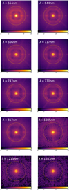 |
Fig. 1 Total intensity in the ten different filters. λ is the central wavelength of each filter. North is up and east to the left. Units are W m−2 sr−1. The dashed orange and white circles mark angular sizes of 500 and 60 ms, respectively. |
Central wavelength, DIT × NDIT (number of DITs), seeing, and airmass for the Betelgeuse exposures as well as the full width at half maximum (FWHM) and SRs measured from the Phi2 Ori images.
3 Analysis
The final reduced images of Stokes Q and U and the linearly polarized intensities, PI, are shown in Fig. 2. The PI images exhibit an overall ring-like structure, compatible with a spherical dust shell seen in polarized light. It is noteworthy that PI drops in the center of images, which is expected for dusty environments observed with scattering angles close to 0°. This is also expected because the positive and negative Q and U signals cancel each other out in this part of the image due to the finite spatial resolution. The AoLP is oriented azimuthally in all filters. Most of the signal is included in a 60 mas radius and peaks at a distance of 30–40 mas from the center (Fig. 4). Along this ring, there is a high azimuthal variation that is consistent over the visible filters. In the near-infrared, the azimuthal profile is much smoother owing to the lower spatial resolution of the images. To illustrate this, we identified four azimuthal sectors of PI values included between a distance of 22 and 60 mas. We plot their variation as a function of azimuth and wavelength in Fig. 5. The highest relative azimuthal variation (with respect to the average value over the same filter) is about 80% and is observed in the Ha-NB filter. The PI mean values vary from sector to sector, with a similar behavior at all wavelength, which indicates azimuthal density variations. This also suggests the components of the polarizing structure are similar, which in terms of dust population could point to a uniform composition and a similar grain size distribution for the four sectors.
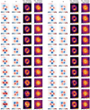 |
Fig. 2 Stokes Q and U and polarized intensity images for the ten filters. The left and right parts correspond to the data before and after Qϕ and Uϕ minimizations, respectively. Red and blue circles represent the photospheric radius (22 mas; Montargès et al. 2016) and the position of the IDS in H2019 (32 mas), respectively. On the polarized intensity map, angles of polarization are marked as orange segments. North is up, and east is to the left. Units are W m−2 sr−1. |
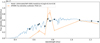 |
Fig. 3 Synthetic flux density (ATLAS9 model with CCM reddening law) and derived flux density from SPHERE observations. The black dots represent the ATLAS9 average flux densities in SPHERE filters. As the conditions did not allow us to trust the ZIMPOL (visible) photometric calibrator measurements, we used the synthetic model fitted in the near-infrared to perform the photometric calibration. |
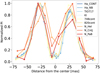 |
Fig. 4 Normalized vertical cut of the polarized intensities in each Alter. |
4 Centro-symmetrical modeling
In order to derive physical parameters from our observations, we compared the SPHERE images to MCFOST (Pinte et al. 2006, 2009) radiative transfer simulations (similarly to H2019). We convolved radiative transfer models with a PSF that was extracted from SPHERE observations of Phi2 Ori in the same instrumental and atmospheric stability conditions. We chose not to model the degree of linear polarization as the intensity at the IDS location is highly contaminated by the stellar flux. For the same reason, we did not model the total intensity images either, as an accurate modeling of the PSF would be very challenging in our case. Our modeling approach is to reproduce the absolute values of the PI signal from the circular structure whose average radius is located at 30 mas. As a first approximation, we modeled the shape seen in the PI images as a spherical shell composed of spherical dust grains. The main parameters of the model are:
a distance of 222 pc (Harper et al. 2017);
an effective stellar temperature of 3600 K (Levesque & Massey 2020);
a stellar radius of 1000 R⊙ (roughly 22 mas photospheric diameter at 222 pc; Montargès et al. 2016);
a stellar mass of 15 M⊙, compatible with mass ranges published in the literature, for example Luo et al. (2022);
an internal and external shell radii (Rin, Rout);
a dust mass (Md);
a size distribution for spherical dust grains between a minimum and a maximum value (amin and amax). We assumed a power law with two values for its index (aexp = 0 and the commonly adopted value from interstellar medium studies: aexp = −3.5; Mathis et al. 1977) and a growth scenario where small grains are always present in the distribution: we set amin to 0.05 µm;
dust composition: we chose enstatite (MgSiO3)as it is the dust species favored by modeling done in H2019. The optical constants of the enstatite are derived from Jäger et al. (2003) and taken from the Jena University Database2. We used the Mie theory to compute optical properties.
As the shell is optically thin, Md acts as a scaling factor to the absolute value of the polarized intensity. It does not influence the geometrical extent of the modeled dust shell. We fixed its value to Md = 10−12M⊙. We ran a grid of MCFOST models to explore the remaining parameters, Rin, Rout, and amax:
amax ranged from 0.1 to 1.1 µm with steps of 0.1 µm;
Rin ranged from 5 AU (roughly the stellar radius) to 15 AU, with a step of 1 AU;
Rout was set to always be higher than Rin by at least 1 AU and up to a maximum of 11 AU (2.25 stellar radii), with a step of 1 AU.
We then computed a χ2 value for each average value per sector compared to the ones extracted from the SPHERE images. We took the median of the χ2 values across the nine filters and plotted it as a function of the grid parameters. Finally, similarly to an analysis presented in Sect. 4.4 of Pinte et al. (2008), we computed a probability for each point of the parameter space (i.e., one model) as  . All probabilities were normalised so that the sum of the probabilities of all models over the entire grid is equal to 1. These results are presented in Fig. 6 and were obtained by marginalising (i.e., summing) the probabilities of all models where one parameter is fixed successively to its different values, that is to say, the probabilities of our 3D parameter space are projected successively on each of the dimensions. Potential correlations between parameters are entirely accounted for with this approach, and the error bars extracted from the probability curves take the interplay between parameters into account.
The models that yield the highest probabilities are presented in Table 2. Whatever the sector, there is an overall decreasing probability for increasing Rin values. This statement is valid to a lesser extent for the Rout distribution of probability because the 1–6 AU range presents important variations, which points to some degree of indetermination for this parameter. The best models in terms of probability have the same extension for all sectors: between 6 and 8 AU (1.2 and 1.6 stellar radius, approximatively). The distribution of amax peaks between 0.4 and 0.6µm, and the best models all have values of 0.5 or 0.6µm. The probability distribution of Rin indicates that the dust shell would start right above the photosphere, where the presence of dust is hard to justify given the high temperatures (see Sect. 5.1). A Rin value of 5 AU corresponds approximately to the full width at half maximum of the PSF that we achieved in these observations (Table 1). Therefore, the estimation of Rin is probably sensitive to convolution effects.
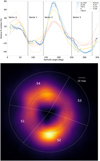 |
Fig. 5 Variation in the PI in the azimuthal direction. Top: azimuthal variation in the PI between 22 and 60 mas. Bottom: image at 717 nm, showing the four sectors. |
Best model parameters by sectors for all models and models whose temperature is below 1500 K.
5 Discussion
5.1 Dust temperature
Despite the relative agreement with observations, the range of dust grain temperature is uncomfortably high for some MgSiO3 models. Figure 7 shows the temperature as a function of distance to the star. Models with distances to the star center of less than 8 AU (~ 1.6 stellar radius) imply grain dust temperatures higher than 1500 K, which is approximatively the MgSiO3 sublimation temperature. These models are consequently not entirely plausible even if they produce a reasonable fit to the SPHERE observations.
Discarding these, the remaining models lead to the distribution of probabilities plotted in blue in Fig. 6. The corresponding best models are summarized in Table 2. The inner radius, Rin, is set to start from 8 AU due to the temperature constraint, and this value corresponds to the Rin for the best models except for sector 3 (9 AU). As noted above, the outer dust shell radius, Rout, is not clearly constrained. For models with a dust temperature lower than 1500 K, this is particularly true for sectors 1 and 2, where the best models have Rout = 12 AU. It is noteworthy that the second-best models for sectors 1 and 2 are the best models for 3 and 4, with Rout = 10 and 9 AU, respectively. All these models systematically have the same maximum size for the grain distribution (amax): 0.6 µm. Absolute normalized values of residuals (or relative difference) for these models are shown as 1D profiles in Fig. 8. The highest absolute values of residuals are reached for the 0.820 µm filter and longer central wavelength filters. This suggests a more complex dust population than what was simulated in our grid of enstatite dust models. Below this wavelength, residuals are below 70% for all sectors. In order to illustrate the departure from spherical symmetry, we show observation, model, and residual images for the best model with T < 1500K, corresponding to sector 2 in Fig. 9. We believe it is possible to reproduce the azimuthal variations with an appropriate 3D density structure. However, this task is beyond the scope of the present paper.
Different structures are present in the first stellar radii: a lukewarm chromosphere (Lim et al. 1998; О’Gorman et al. 2017) whose temperature at 1.7 stellar radius is about 3000 K (Fig. 4 in О’Gorman et al. 2020), a 2000–2500 K MOL sphere at about 1.3 stellar radius (Perrin et al. 2004; Tsuji 2006; Ohnaka et al. 2011; Montargès et al. 2014), and the inner dust environment that we focus on in the present paper. O’Gorman et al. (2020, Sect. 4.1) propose that the coexistence of different temperatures can be reconciled if the different components are distributed in small inhomogeneities, smaller than the angular resolution. For an IDS at 1.5 stellar radius, the local temperature needs to allow dust survival; these inhomogeneous dusty zones would be preferably found above the coolest areas of the convective surface.
The radial location and morphology of the azimuthal IDS structures reported here are similar to the features of the 28SiO emission line intensity map presented in Fig. 5 of Kervella et al. (2018) from 2016 ALMA observations. They are both included within the first 3 stellar radii (~15AU, ~66 mas) and present arc-shaped structures. The exact connection between the structures on the two maps is not clear as condensation times and the dynamics at play are not known. Nevertheless, having such a distribution of gaseous SiO in the immediate circumstellar environment supports an at least partial silicate composition for the IDS, which is also compatible with predictions of the thermodynamical calculations of dust condensation in Betelgeuse (Gupta & Sahijpal 2020).
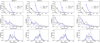 |
Fig. 6 Probabilities of the various parameters for two values of aexp per sector for the whole range of models (black) and for models whose dust temperatures do not exceed 1500 K (blue). The triangles represent the parameters of the best model for each case. |
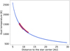 |
Fig. 7 Dust grain temperature as a function of distance for the best models of the four sectors. The red segment of the curves marks the zone where the grain dust density is located. |
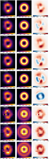 |
Fig. 9 Polarized intensity images. Left: observed images in polarized intensity. Middle: best model with dust temperatures below 1500 K for sector 2. Right: residuals (observation minus model). |
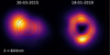 |
Fig. 10 Evolution of the IDS in polarized intensity. Images are not deconvolved, and the convention is the same as in Fig. 2. |
5.2 Mass loss
The amount of dust mass reported here, le-12M⊙, is significantly lower than the IDS mass of 1.5e-10M⊙ reported in H2019 and the dust mass-loss rate of 2e-9 M⊙yr−1 reported in Josselin & Plez (2007). As noted above, it is possible that the actual IDS mass needed to reproduce the asymmetric features is much higher. It should also be noted that we have not probed models involving nonspherical dust particles and that results presented here could also vary with a larger exploration of dust properties.
It is also possible that the IDS exhibits variability with a minimum timescale of years. This is supported by the morphological variation in the IDS between observations reported in Kervella et al. (2016, however, the non-deconvolved PI images were not published) and the observations reported here, which are shown in Fig. 10. In both images, most of the polarized flux is enclosed within a ~70 mas radius and the maximum is found ~30 mas from the center. However, the spatial distributions of the intensity at the two epochs differ significantly in both radial and azimuthal directions. In the 2015 image, there is a significant polarized flux emission within the photospheric (red) radius, whereas in 2019 this area is characterized by a drop, creating a globally more ring-like structure than in 2015.
6 Conclusion
We have presented polarimetric high-spatial-resolution images of the Betelgeuse IDS obtained with SPHERE/ZIMPOL and SPHERE/IRDIS. Within our modeling hypotheses, the polarized signal arises from stellar light scattered by a centro-symmetric dust shell that extends up to several AUs above the photosphere. Following H2019, we assumed dust grains are composed of MgSiO3 and that the derived maximum dust grain size is in the 0.4–0.6 µm range, 0.6 µm for the best-fitting model. Though our modeling is limited, the description it gives of the polarized structure around Betelgeuse in terms of grain size distribution did not show any great variation between 2013 (reported in H2019) and 2019. It is possible that this points to a relatively stable dust condensation radius and dust characteristics over time. Our centro-symmetric model leads to large azimuthal residuals that may be the results of density variations, for instance due to asymmetric outflows, projection effects, and/or illumination asymmetries. In order to further constrain the mechanisms at play in this IDS, further work should include a modeling of these effects as well as a monitoring of the IDS, whose morphology is believed to vary over several months to 1 yr. This should allow the links between the IDS and surface phenomena, which vary on similar timescales, to be revealed.
Acknowledgements
This work has made use of the SPHERE Data Centre, jointly operated by OSUG/IPAG (Grenoble), PYTHEAS/LAM/CESAM (Marseille), OCA/Lagrange (Nice), Observatoire de Paris/LESIA (Paris), and Observatoire de Lyon.
References
- Avenhaus, H., Quanz, S. P., Schmid, H. M., et al. 2014, ApJ, 781, 87 [Google Scholar]
- Beuzit, J. L., Vigan, A., Mouillet, D., et al., 2019, A&A, 631, A155 [NASA ADS] [CrossRef] [EDP Sciences] [Google Scholar]
- Bordé, P., Coudé du Foresto, V., Chagnon, G., et al. 2002, A&A, 393, 183 [CrossRef] [EDP Sciences] [Google Scholar]
- Canovas, H., Ménard, F., de Boer, J., et al. 2015, A&A, 582, A7 [Google Scholar]
- Cardelli, J. A., Clayton, G. C., & Mathis, J. S. 1989, ApJ, 345, 245 [Google Scholar]
- Castelli, F., & Kurucz, R. L. 2003, Modell. Stellar Atmos., 210, A20 [Google Scholar]
- Cohen, M., Walker, R. G., Carter, B., et al. 1999, AJ, 117, 1864 [Google Scholar]
- de Boer, J., Langlois, M., van Holstein, R. G., et al. 2020, A&A, 633, A63 [NASA ADS] [CrossRef] [EDP Sciences] [Google Scholar]
- Delorme, P., Meunier, N., Albert, D., et al. 2017, SF2A-2017: Proceedings of the Annual meeting of the French Society of Astronomy and Astrophysics [Google Scholar]
- Dohlen, K., Langlois, M., Saisse, M. et al. 2008, SPIE Conf. Ser., 7014, 1266 [Google Scholar]
- Dupree, A. K., Strassmeier, K. G., Matthews, L. D., et al. 2020, ApJ, 899, 68 [Google Scholar]
- Gail, H.-P., Tamanai, A., Pucci, A., et al. 2020, A&A, 644, A139 [NASA ADS] [CrossRef] [EDP Sciences] [Google Scholar]
- Gupta, A., & Sahijpal, S. 2020, MNRAS, 496, L122 [NASA ADS] [CrossRef] [Google Scholar]
- Harper, G. M., Brown, A., Guinan, E. F., et al. 2017, AJ, 154, 11 [Google Scholar]
- Harper, G. M., Guinan, E. F., Wasatonic, R., et al. 2020, ApJ, 905, 34 [CrossRef] [Google Scholar]
- Haubois, X., Norris, B., Tuthill, P. G., et al. 2019, A&A, 628, A101 [NASA ADS] [CrossRef] [EDP Sciences] [Google Scholar]
- Jäger, C., Dorschner, J., Mutschke, H., Posch, T., & Henning, T. 2003, A&A, 408, 193 [NASA ADS] [CrossRef] [EDP Sciences] [Google Scholar]
- Josselin, E., & Plez, B. 2007, A&A, 469, 671 [NASA ADS] [CrossRef] [EDP Sciences] [Google Scholar]
- Kervella, P., Perrin, G., Chiavassa, A., et al. 2011, A&A, 531, A117 [NASA ADS] [CrossRef] [EDP Sciences] [Google Scholar]
- Kervella, P., Lagadec, E., Montargès, M., et al. 2016, A&A, 585, A28 [NASA ADS] [CrossRef] [EDP Sciences] [Google Scholar]
- Kervella, P., Decin, L., Richards, A. M. S., et al. 2018, A&A, 609, A67 [NASA ADS] [CrossRef] [EDP Sciences] [Google Scholar]
- Kravchenko, K., Jorissen, A., Van Eck, S., et al. 2021, A&A, 650, A17 [NASA ADS] [CrossRef] [EDP Sciences] [Google Scholar]
- Levesque, E. M., & Massey, P. 2020, ApJ, 891, L37 [Google Scholar]
- Lim, J., Carilli, C. L., White, S. M., et al. 1998, Nature, 392, 575 [NASA ADS] [CrossRef] [Google Scholar]
- Luo, T., Umeda, H., Yoshida, T., et al. 2022, ApJ, 927, 115 [CrossRef] [Google Scholar]
- Mathis, J. S., Rumpl, W., & Nordsieck, K. H. 1977, ApJ, 217, 425 [Google Scholar]
- Milli, J., Kasper, M., Bourget, P., et al. 2018, Proc. SPIE, 10703, 107032A [Google Scholar]
- Montargès, M., Kervella, P., Perrin, G., et al. 2014, A&A, 572, A17 [NASA ADS] [CrossRef] [EDP Sciences] [Google Scholar]
- Montargès, M., Kervella, P., Perrin, G., et al. 2016, A&A, 588, A130 [NASA ADS] [CrossRef] [EDP Sciences] [Google Scholar]
- Montargès, M., Cannon, E., Lagadec, E., et al. 2021, Nature, 594, 365 [Google Scholar]
- Nozawa, T., Maeda, K., Kozasa, T., et al. 2011, ApJ, 736, 45 [NASA ADS] [CrossRef] [Google Scholar]
- O’Gorman, E., Kervella, P., Harper, G. M., et al. 2017, A&A, 602, A10 [Google Scholar]
- O’Gorman, E., Harper, G. M., Ohnaka K., et al. 2020, A&A, 638, A65 [NASA ADS] [CrossRef] [EDP Sciences] [Google Scholar]
- Ohnaka, K., Weigelt, G., Millour, F., et al. 2011, A&A, 529, A163 [NASA ADS] [CrossRef] [EDP Sciences] [Google Scholar]
- Perrin, G., Ridgway, S. T., Coudé du Foresto, V., et al. 2004, A&A, 418, 675 [NASA ADS] [CrossRef] [EDP Sciences] [Google Scholar]
- Perrin, G., Verhoelst, T., Ridgway, S. T., et al. 2007, A&A, 474, 599 [NASA ADS] [CrossRef] [EDP Sciences] [Google Scholar]
- Pinte, C., Ménard, F., Duchêne, G., & Bastien, P. 2006, A&A, 459, 797 [NASA ADS] [CrossRef] [EDP Sciences] [Google Scholar]
- Pinte, C., Padgett, D. L., Ménard, F., et al. 2008, A&A, 489, 633 [NASA ADS] [CrossRef] [EDP Sciences] [Google Scholar]
- Pinte, C., Harries, T. J., Min, M., et al. 2009, A&A, 498, 967 [NASA ADS] [CrossRef] [EDP Sciences] [Google Scholar]
- Roddier, F., & Roddier, C. 1985, ApJ, 295, L21 [NASA ADS] [CrossRef] [Google Scholar]
- Safonov, B., Dodin, A., Burlak, M., et al. 2020, ArXiv e-prints [arXiv:2005.05215] [Google Scholar]
- Schmid, H. M., Bazzon, A., Roelfsema, R., et al. 2018, A&A, 619, A9 [NASA ADS] [CrossRef] [EDP Sciences] [Google Scholar]
- STScI Development Team 2013, Astrophysics Source Code Library, [record ascl:1303.023] [Google Scholar]
- Taniguchi, D., Yamazaki, K., & Uno, S. 2022, Nat. Astron., 6, 930 [NASA ADS] [CrossRef] [Google Scholar]
- Tsuji, T. 2006, ApJ, 645, 1448 [Google Scholar]
- van Holstein, R. G., Snik, F., Girard, J. H., et al. 2017, SPIE Conf. Ser., 10400, 1040015 [Google Scholar]
- van Holstein, R. G., Girard, J. H., de Boer, J., et al. 2020, A&A, 633, A64 [NASA ADS] [CrossRef] [EDP Sciences] [Google Scholar]
- Verhoelst, T., Decin, L., van Malderen, R., et al. 2006, A&A, 447, 311 [NASA ADS] [CrossRef] [EDP Sciences] [Google Scholar]
https://irdap.readthedocs.io (IRDIS Data reduction for Accurate Polarimetry).
All Tables
Central wavelength, DIT × NDIT (number of DITs), seeing, and airmass for the Betelgeuse exposures as well as the full width at half maximum (FWHM) and SRs measured from the Phi2 Ori images.
Best model parameters by sectors for all models and models whose temperature is below 1500 K.
All Figures
|
Fig. 1 Total intensity in the ten different filters. λ is the central wavelength of each filter. North is up and east to the left. Units are W m−2 sr−1. The dashed orange and white circles mark angular sizes of 500 and 60 ms, respectively. |
| In the text | |
|
Fig. 2 Stokes Q and U and polarized intensity images for the ten filters. The left and right parts correspond to the data before and after Qϕ and Uϕ minimizations, respectively. Red and blue circles represent the photospheric radius (22 mas; Montargès et al. 2016) and the position of the IDS in H2019 (32 mas), respectively. On the polarized intensity map, angles of polarization are marked as orange segments. North is up, and east is to the left. Units are W m−2 sr−1. |
| In the text | |
|
Fig. 3 Synthetic flux density (ATLAS9 model with CCM reddening law) and derived flux density from SPHERE observations. The black dots represent the ATLAS9 average flux densities in SPHERE filters. As the conditions did not allow us to trust the ZIMPOL (visible) photometric calibrator measurements, we used the synthetic model fitted in the near-infrared to perform the photometric calibration. |
| In the text | |
|
Fig. 4 Normalized vertical cut of the polarized intensities in each Alter. |
| In the text | |
|
Fig. 5 Variation in the PI in the azimuthal direction. Top: azimuthal variation in the PI between 22 and 60 mas. Bottom: image at 717 nm, showing the four sectors. |
| In the text | |
|
Fig. 6 Probabilities of the various parameters for two values of aexp per sector for the whole range of models (black) and for models whose dust temperatures do not exceed 1500 K (blue). The triangles represent the parameters of the best model for each case. |
| In the text | |
|
Fig. 7 Dust grain temperature as a function of distance for the best models of the four sectors. The red segment of the curves marks the zone where the grain dust density is located. |
| In the text | |
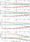 |
Fig. 8 Residuals per sector as defined in Fig. 5. |
| In the text | |
|
Fig. 9 Polarized intensity images. Left: observed images in polarized intensity. Middle: best model with dust temperatures below 1500 K for sector 2. Right: residuals (observation minus model). |
| In the text | |
|
Fig. 10 Evolution of the IDS in polarized intensity. Images are not deconvolved, and the convention is the same as in Fig. 2. |
| In the text | |
Current usage metrics show cumulative count of Article Views (full-text article views including HTML views, PDF and ePub downloads, according to the available data) and Abstracts Views on Vision4Press platform.
Data correspond to usage on the plateform after 2015. The current usage metrics is available 48-96 hours after online publication and is updated daily on week days.
Initial download of the metrics may take a while.