| Issue |
A&A
Volume 678, October 2023
|
|
|---|---|---|
| Article Number | A81 | |
| Number of page(s) | 10 | |
| Section | The Sun and the Heliosphere | |
| DOI | https://doi.org/10.1051/0004-6361/202347466 | |
| Published online | 10 October 2023 | |
Influence of the interstellar magnetic field and 11-year cycle of solar activity on the heliopause nose location
Space Research Centre Polish Academy of Sciences, Bartycka 18A, 00-716 Warsaw, Poland
e-mail: This email address is being protected from spambots. You need JavaScript enabled to view it.
Received:
14
July
2023
Accepted:
9
August
2023
Abstract
Context. The heliosphere is formed by the interaction between the solar wind (SW) plasma emanating from the Sun and a magnetised component of local interstellar medium (LISM) inflowing on the Sun. A separation surface called the heliopause (HP) forms between the SW and the LISM.
Aims. In this article, we define the nose of the HP and investigate the variations in its location. These result from a dependence on the intensity and direction of the interstellar magnetic field (ISMF), which is still not well known but has a significant impact on the movement of the HP nose, as we try to demonstrate in this paper.
Methods. We used a parametric study method based on numerical simulations of various forms of the heliosphere using a time-dependent three-dimensional magnetohydrodynamic (3D MHD) model of the heliosphere.
Results. The results confirm that the nose of the HP is always in a direction that is perpendicular to the maximum ISMF intensity directly behind the HP. The displacement of the HP nose depends on the direction and intensity of the ISMF, with the structure of the heliosphere and the shape of the HP depending on the 11-year cycle of solar activity.
Conclusions. In the context of the planned space mission to send the Interstellar Probe (IP) to a distance of 1000 AU from the Sun, our study may shed light on the question as to which direction the IP should be sent. Further research is needed that introduces elements such as current sheet, reconnection, cosmic rays, instability, or turbulence into the models.
Key words: Sun: heliosphere / interplanetary medium / magnetohydrodynamics (MHD) / Sun: magnetic fields / solar wind / ISM: magnetic fields
© The Authors 2023
 Open Access article, published by EDP Sciences, under the terms of the Creative Commons Attribution License (https://creativecommons.org/licenses/by/4.0), which permits unrestricted use, distribution, and reproduction in any medium, provided the original work is properly cited.
This article is published in open access under the Subscribe to Open model. This email address is being protected from spambots. You need JavaScript enabled to view it. to support open access publication.
1. Introduction
The interaction of the supersonic solar wind (SW) with the local interstellar medium (LISM) leads to the formation of a cavity in the LISM called the heliosphere, which is filled with the SW plasma. The interaction between the SW plasma outflowing spherically and symmetrically from the Sun and the counter-flowing LISM plasma in a uniform rectilinear motion, and neglecting the magnetic fields in both media, results in the axisymmetric shape of the heliosphere. The axial symmetry of the heliosphere also holds when the direction of the interstellar magnetic field (ISMF) is the same as that of the LISM inflow, if the interplanetary magnetic field (IMF) is neglected. Mathematically speaking, the heliosphere is separated from the LISM by the heliopause (HP), a discontinuity surface that is the pressure equilibrium surface of both media. The supersonic SW slows down before the HP through a shock wave called the termination shock (TS). If the interstellar plasma is also supersonic, it slows down on the other side of HP through a shock wave known as a bow shock (BS). The area between the TS and the HP is an inner heliosheath (IHS). A layer located between the HP and the BS is an outer heliosheath (OHS), if the BS exists. Otherwise, the OHP between the HP and the region where the LISM is disturbed by the heliosphere causes flowing around the HP. In this way, the SW plasma flows around the inner part of the HP, and the LISM plasma flows around the outer part of the HP (Fig. 1). In an axisymmetric heliosphere, a line running through the centre of the Sun and parallel to the velocity vector of the LISM intersects the surfaces of the TS, HP, and BS at points that are called the noses of the TS, HP, and BS (Fig. 1).
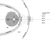 |
Fig. 1. Schematic of the IHS and OHS in the parallel LISM velocity and magnetic field vectors (axisymmetric case). The TS, HP, and BS noses are on one line. |
When we include the ISMF Bis, not parallel to the LISM velocity vector Vis, the noses of TS, HP, and BS change positions (Fig. 2). The noses of the TS and HP deflect in one direction and the nose of the BS deflects in the other direction (Fig. 2) (compare with Ratkiewicz et al. 1998, 2000).
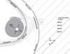 |
Fig. 2. Schematic of the heliosphere and LISM for an ISMF not parallel to the LISM velocity vector. The TS and HP noses deviate in one direction (quasi-perpendicular to the undisturbed Bis), and the BS nose in the opposite direction (Ratkiewicz et al. 2000). |
The nose of the heliosphere is cited in various contexts in many publications. In some, the nose is identified with the stagnation point of the interstellar medium flow (e.g., Drake et al. 2010; Desai et al. 2015; Dayeh et al. 2019; McComas et al. 2020; Shrestha et al. 2023). Many articles refer to the HP nose as ‘the nose region of the heliosheath’, ‘the nose of the heliosphere’ (e.g., McComas & Schwadron 2006; Lee et al. 2009; Fisk & Gloeckler 2009, 2014, 2015; Galli et al. 2019; Kornbleuth et al. 2020, 2021a; Opher et al. 2017; Shrestha et al. 2023), ‘the nose direction’ (e.g., Müller et al. 2008; Opher & Drake 2013; Opher et al. 2015, 2017, 2021; Zirnstein et al. 2020) or ‘the upwind (nose) direction’ (e.g., McComas et al. 2020; Kornbleuth et al. 2021b). However, relatively little attention has been paid to the consideration of the location of the heliosphere nose, more precisely the location of the noses of the TS, HP, and BS and the displacement of the nose. This issue was first addressed in the 1980s, using the so-called Newtonian approximation as a model of the heliosphere (see Figs. 2 and 3 Fahr et al. 1986, 1988; Ratkiewicz & Banaszkiewicz 1987; Banaszkiewicz & Ratkiewicz 1989). Recently, this issue has been revisited in (Ratkiewicz & Baraniecka 2023), where the HP nose is defined in Fig. 2. The above articles show that the location of the HP nose depends upon the direction and intensity of the ISMF and always deflects in a direction quasi-perpendicular to the direction of the undisturbed ISMF lines (Ratkiewicz et al. 2000).
In this article, using the definition of the HP nose in Fig. 1 (compare with Fig. 2 in Ratkiewicz & Baraniecka 2023), we discuss possible configurations of the HP nose, arising under the influence of various ISMF intensities and directions, for the SW velocity during the minimum and maximum of the 11-year cycle of solar activity, (Fig. 3). We show that the HP nose clearly deviates from the LISM inflow direction and is always directed towards the ISMF maximum, just behind the HP.
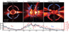 |
Fig. 3. Adapted Figs. 1(a–d) from McComas et al. (2008), original caption ‘(a–c) Polar plots of the solar wind speed, colored by IMF polarity for Ulysses’ three polar orbits colored to indicate measured magnetic polarity. In each, the earliest times are on the left (nine o’clock position) and progress aroundcounterclockwise. (d) Contemporaneous values for the smoothed sunspot number (black) and heliospheric current sheettilt (red), lined up to match Figs. 1a–c. In Figs. 1a–c, the solar wind speed is plotted over characteristic solarimages for solar minimum for cycle 22 (8/17/96), solar maximum for cycle 23 (12/07/00), and solar minimum for cycle 23(03/28/06). From the center out, we blend images from the Solar and Heliospheric Observatory (SOHO) Extremeultraviolet Imaging Telescope (Fe XII at 1950 nm), the Mauna Loa K coronameter (700–950 nm), and the SOHO C2white light coronagraph. |
The paper is organised as follows: in Sect. 2, we describe the simulation method and three sets of boundary conditions; in Sect. 3, we present the results of our modelling; in Sect. 4, we present our conclusions.
2. Simulation method and boundary conditions
We used a three-dimensional (3D) magnetohydrodynamic (MHD) model of the interaction between the SW and LISM, as described by Ratkiewicz et al. (2002, 2008), with a number of revisions introduced, including: a magnetised SW, the boundary conditions adjusted to simulate solar cycle effects, and an improved modelling of the neutral hydrogen within the constant flux approximation, as described by Strumik & Ratkiewicz (2022). The set of MHD equations in Eq. (1) includes a source term S on the right-hand side to describe a resonance charge exchange with a constant flux of hydrogen, and a second source term, Q, that maintains the divergence-free magnetic field (Ratkiewicz et al. 2002, 2008).
 (1)
(1)
where U, Q, and S are column vectors, and  is a flux tensor defined as
![Mathematical equation: $$ \begin{aligned} \boldsymbol{U}&= \left[ \begin{array}{c} \rho \\ \rho \boldsymbol{u} \\ \boldsymbol{B} \\ \rho E \end{array} \right], \hat{\boldsymbol{F}} = \left[ \begin{array}{c} \rho \boldsymbol{u} \\ \rho \boldsymbol{uu} + \boldsymbol{I}\left(p + \frac{\boldsymbol{B \cdot B}}{8 \pi }\right) - \frac{\boldsymbol{BB}}{4\pi } \\ \boldsymbol{uB} - \boldsymbol{Bu} \\ \rho \mathrm{H}\boldsymbol{u} - \frac{\boldsymbol{B}(\boldsymbol{u} \cdot \boldsymbol{B})}{4\pi } \end{array} \right], \\ \boldsymbol{Q}&= - \left[ \begin{array}{c} 0 \\ \frac{\boldsymbol{B}}{4\pi } \\ \boldsymbol{u} \\ \boldsymbol{u} \cdot \frac{\boldsymbol{B}}{4\pi } \end{array} \right] \nabla \cdot \boldsymbol{B}, \boldsymbol{S} = \rho \nu _{\rm c} \left[ \begin{array}{c} 0 \\ \boldsymbol{V}_{\rm H} - \boldsymbol{u} \\ 0 \\ \frac{1}{2} V_{\rm H}^2 + \frac{3k_{\rm B}T_{\rm H}}{2m_{\rm H}} - \frac{1}{2}u^2-\frac{k_{\rm B}T}{(\gamma - 1)m_{\rm H}} \end{array} \right] \end{aligned} $$](/articles/aa/full_html/2023/10/aa47466-23/aa47466-23-eq3.gif)
Here, ρ is the ion mass density, p = 2nkBT is the pressure, n is the ion number density, T and TH (TH = const.) are ion and hydrogen atom temperatures, u and VH (VH = const.) are the ion and hydrogen atom velocity vectors, respectively, B is the magnetic field vector,  is the total energy per unit mass, and
  is enthalpy. The γ is the ratio of specific heats and I is the 3 × 3 identity matrix. The charge exchange collision frequency is νc = nHσus, where nH (nH = const.) is the hydrogen atom number density, σ is the charge exchange cross-section, and
  is the effective average relative speed of protons and hydrogen atoms, assuming a Maxwellian spread of velocities both for protons and hydrogen atoms. The flows are taken to be adiabatic, with
  . The additional constraint of a divergence-free magnetic field, ∇ ⋅ B = 0, in the numerical simulations is accomplished by adding the source term Q to the right-hand side of (Eq. (1)), which is proportional to the divergence of the magnetic field. Adding Q to the right-hand side of (Eq. (1)) assures that any numerically generated ∇ ⋅ B ≠ 0 is advected with the flow, and allows one to limit the growth of ∇ ⋅ B ≠ 0.
In order to thoroughly analyse the movement of the nose HP, we considered three cases:
The LISM parameters are set at the outer boundary, 5000 AU from the Sun: velocities and temperatures of ionised and neutral LISM components are equal and Vis = 26.4 km s−1, Tis = 6400 K, proton number density np = 0.06 cm−3, and neutral hydrogen number density nH = 0.11 cm−3.
The SW parameters are set at the inner boundary, 10 AU from the Sun: In case one, velocity Vsw = 420 km s−1, number density SW protons np = 0.052 cm−3, and the IMF is neglected. In case two, Vsw and nsw are the same as case one, but the IMF is set according to the Parker model as an Archimedean spiral, and its strength at 1 AU equals 35.5 μG. In case three, for the slow SW, velocity Vsw = 420 km s−1, number density np = 0.052 cm−3; for the fast SW, velocity Vsw = 798 km s−1, number density np = 0.027 cm−3; the IMF for the slow and fast SW is the same as case two.
To show the effect of the ISMF intensity and direction on the deviation of the HP nose from the direction of the LISM inflow, we considered different HP configurations for the ISMF intensities of 2 μG, 3 μG, and 4 μG and for the angle between the LISM velocity vector and the direction of the ISMF vector, called an inclination angle α, 0°, 30°, 60°, and 90°.
3. Results
3.1. The behaviour of the HP in the case of LISM velocity parallel to the ISMF
The HP shape and HP nose for the three cases of intensity of the ISMF with the ISMF direction parallel to the LISM velocity vector are shown in Figs. 4a–c.
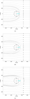 |
Fig. 4. HP shape and location of the noses of the HP. Velocity streamlines for inclination angle equal 0° are shown in the x − y plane (a) ISMF intensity equal to 2 μG (b) ISMF intensity equal to 3 μG (c) ISMF intensity equal to 4 μG. |
For the ISMF parallel to the LISM velocity, the heliosphere is axisymmetric, so in the x − y and x − z planes it looks the same and in the y − z plane, the isolines form circles with the Sun in the centre (compare with Figs. 3a–c Ratkiewicz et al. 2000). As shown in Figs. 4a–c, the characteristic feature for various ISMF intensities is that the more the ISMF compresses the HP, the greater the ISMF intensity is. The HP nose is in each case located at the intersection of the x-axis with the HP (blue dots). On the other hand, the greater the ISMF intensity, the farther the HP nose is from the Sun, so that, in the case of an ISMF parallel to the LISM velocity vector, the greater the ISMF intensity, the farther the HP nose is extended towards the direction of the interstellar medium.
3.2. The behaviour of the HP in the case of LISM velocity perpendicular to the ISMF
The heliosphere for case one, iso without IMF, of the ISMF direction perpendicular to the LISM velocity is shown in the x − y, x − z, and y − z planes in Figs. 5a–c for an ISMF intensity of 4 μG to illustrate the shape of the HP and the nose location.
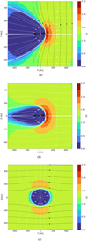 |
Fig. 5. Velocity streamlines (white) and magnetic fieldlines (black) shown for the ISMF magnitude for the inclination angle equal to 90° and for ISMF intensity 4 μG, without the IMF (a) x − y plane (b) x − z plane (note, magnetic fieldlines in this case are perpendicular to x − z plane and are omitted) (c) y − z plane. |
For an ISMF perpendicular to the LISM velocity, the heliosphere (in comparison to the parallel field described above) loses its axial symmetry. In the x − y plane, the nose of the HP, squeezed by the perpendicular lines of the ISMF field, approaches the Sun (see Fig. 5a), and the profile of the HP towards its tail increases its distance from the Sun. In the x − z plane, the HP is compressed along the z-axis (see Fig. 5b). In the y − z plane (see Fig. 5c), the HP has the shape of a flattened circle (compare with Fig. 4 Ratkiewicz et al. 2000). As can be seen in Figs. 5a–c, the maximum ISMF intensity is in the direction perpendicular to the Sun’s line of sight (compare Ratkiewicz et al. 2000).
Figure 6 shows the same results as Fig. 5a, except for the ISMF intensity, which in Fig. 5a is two times greater (4 μG) than in Fig. 6 (2 μG). This comparison shows the greater compression of the HP nose in Fig. 5a, which is manifested by a shorter distance of the HP nose and the Sun and by greater distances between the heliosphere surface and the x-axis towards the tail.
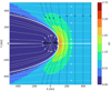 |
Fig. 6. Velocity streamlines (white) and magnetic fieldlines (black) shown for the ISMF magnitude for the inclination angle equal to 90° and for ISMF intensity 2 μG, without the IMF, in the x − y plane. |
3.3. The behaviour of the HP in the case of ISMF direction oblique to the LISM velocity
In numerical simulations, two inclination angles from the range 0° < α < 90° are taken into account, namely, α = 30° and α = 60°. In order to determine the offset of the HP nose, cases one through three (see Sect. 2) were first analysed for the angle α = 60°.
Figures 7a–c show the deviation of the HP nose from the direction of the LISM velocity and the shape of the HP for the ISMF intensity 2 μG using the streamlines. To better analyse the behaviour of the HP nose, comparisons with Figs. 7a–c and 8a–c were created, which show the same results as Figs. 7a–c, but with the use of magnetic fieldlines. It is easy to see that the HP for solar maximum, without an IMF (case one; see Figs. 7a and 8a) is greater than for case two with the IMF (see Figs. 7b and 8b). The heliosphere for the minimum 11-year cycle of solar activity, with the IMF taken into account, (case three; see Figs. 7c and 8c) differs from the previous examples (Figs. 7b and 8b). In all three cases, the nose of the HP clearly deviates from the direction of the LISM velocity.
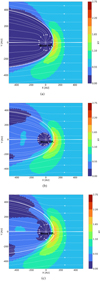 |
Fig. 7. Velocity streamlines (white) shown for the magnetic field magnitude for the inclination angle α = 60° and for ISMF intensity 2 μG (a) Iso SW without the IMF (b) Iso SW with the IMF (c) Anis SW with the IMF. |
The next sequence of figures (9a–c and 10a–c) describes the same results as Figs. 8a–c for an ISMF intensity of 3 μG and 4 μG for α = 60°. Figures 8a, 9a, and 10a (case one) show that the greater the ISMF intensity, the closer the HP nose is to the Sun and the greater the distance of the heliosphere surface from the x-axis towards the tail. It is clear that case one, where an IMF is not included, is different from case two and case three. A comparison of Figs. 8b with 8c, 9b with 9c, and 10b with 10c reveals a different structure of the heliosphere regardless of the ISMF intensity. A comparison of Figs. 8a–c with 9a–c and with 10a–c shows that the greater the ISMF intensity, the greater the distance of the heliosphere surface from the x-axis towards the tail. However, in each case, the nose of the HP clearly deviates from the direction of the LISM velocity perpendicular to the maximum of the ISMF intensity.
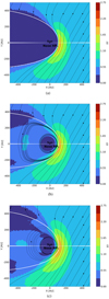 |
Fig. 8. Magnetic fieldlines (black) shown for the magnetic field magnitude for the inclination angle α = 60° and for ISMF intensity 2 μG (a) Iso SW without the IMF (compare to 7a) (b) Iso SW with the IMF (compare to 7b) (c) Anis SW with the IMF (compare to 7c). |
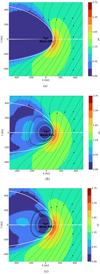 |
Fig. 9. Magnetic fieldlines (black) shown for the magnetic field magnitude for the inclination angle α = 60° and for ISMF intensity 3 μG (a) Iso SW without the IMF (compare to Fig. 8a) (b) Iso SW with the IMF (compare to Fig. 8b) (c) Anis SW with the IMF (compare to Fig. 8c). |
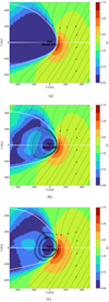 |
Fig. 10. Magnetic fieldlines (black) shown for the magnetic field magnitude for the inclination angle α = 60° and for ISMF intensity 4 μG (a) Iso SW without the IMF (compare to Figs. 8a and 9b) (b) Iso SW with the IMF (compare to Figs. 8c and 9c) (c) Anis SW with the IMF (compare to Figs. 8d and 9e). |
The next sequence of figures, 11a–c, describes case one (iso SW without the IMF) for the ISMF intensity of 2 μG, 3 μG, and 4 μG for α = 30°. Figures 11a–c show that the HP nose for the inclination angle α = 30° deviates from the LISM velocity more than for the angle α = 60° (compare Figs. 8a, 9a, and 10a) regardless of the ISMF intensity (see Fahr et al. 1986, 1988). Furthermore, the heliosphere shape differs for varies ISMF intensity. The next sequence of figures, 12a and b, describe case two (isotropic SW with the IMF) for the ISMF intensity of 3 μG and 4 μG for α = 30°. In case two, Figs. 12a and b, with the IMF and the isotropic SW for inclination angle α = 30° show differences in the heliosphere structures for the ISMF intensities of 3 μG and 4 μG. The next sequence of Figs. 13a and b describes case three (SW with the IMF, anis SW) for the ISMF intensities of 2 μG and 4 μG and the inclination angle of α = 30°. In case three, the Figs. 13a and b, with the IMF, and the anisotropic SW for an inclination angle of α = 30° , show even greater differences in the heliosphere structures for the ISMF intensities of 2 μG and 4 μG.
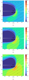 |
Fig. 11. Magnetic fieldlines (black) shown for the magnetic field magnitude for the inclination angle α = 30°, without the IMF, and with iso SW (a) ISMF intensity 2 μG (b) ISMF intensity 3 μG (c) ISMF intensity 4 μG. |
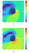 |
Fig. 12. Magnetic fieldlines (black) shown for the magnetic field magnitude for the inclination angle α = 30°, with the IMF, and with iso SW (a) ISMF intensity 3 μG (b) ISMF intensity 4 μG. |
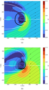 |
Fig. 13. Magnetic fieldlines (black) shown for the magnetic field magnitude for the inclination angle α = 30°, with the IMF, and with anis SW (a) ISMF intensity 2 μG (b) ISMF intensity 4 μG. |
4. Summary and conclusions
The three different models of the heliosphere were created using the 3D MHD numerical program for three different boundary conditions:
-
the interaction of the isotropic SW (maximum of an 11-year solar cycle) with the LISM, without considering the IMF,
-
the interaction of the isotropic SW with the LISM, considering the IMF,
-
the interaction of the anisotropic SW (minimum of an 11-year solar cycle) with the LISM, and considering the IMF.
The purpose of this article is to define the nose of the HP and investigate the differences in its location resulting from a dependence on the intensity and direction of the ISMF, which is still not well known, but which has a significant impact on the HP nose movement, as we have tried to demonstrate in this paper. We explored the differences and similarities between the three models, taking into account the different study setups. We analysed the ISMF direction parallel, perpendicular, and oblique to the LISM velocity vector.
For the ISMF parallel to the LISM velocity, the heliosphere is axisymmetric. What is characteristic in this case is that the more the ISMF compresses the HP, the greater the ISMF intensities are. The HP nose is in each case at the intersection of the x-axis with the HP. Simultaneously, the greater the ISMF intensity, the farther the HP nose is from the Sun (see Figs. 4a–c).
For the ISMF perpendicular to the LISM velocity, the heliosphere loses its axial symmetry. In the x − y plane, the nose of the HP, squeezed by the perpendicular lines of the ISMF field, approaches the Sun, and the profile of the HP towards its tail increases its distance from the Sun. In the x − z plane, the HP is compressed along the z-axis. In the y − z plane, the HP has the shape of a flattened circle. The maximum ISMF intensity is in the direction perpendicular to the Sun’s line of sight (see our Figs. 5a–c and 6 and compare with Ratkiewicz et al. 2000).
In the case of the oblique ISMF direction to the LISM velocity, when α = 60° , the HP for solar maximum without an IMF (case one; see Figs. 7a and 8a) is greater than for case two with the IMF (see Figs. 7b and 8b). The heliosphere for the minimum 11-year cycle of solar activity with the IMF taken into account (case three, see Figs. 7c and 8c) differs from the previous cases (Figs. 7b and 8b). In all three cases, the nose of the HP clearly deviates from the direction of the LISM velocity.
A comparison of Figs. 8a, 9a, and 10a (case one) clearly shows that the greater the ISMF intensity, the closer the HP nose is to the Sun and the greater the distance of the heliosphere surface from the x-axis towards the tail. Figures 11a–c show that the HP nose for the inclination angle α = 30° deviates from the LISM velocity more than for angle α = 60° , regardless of the ISMF intensity (see Fahr et al. 1986, 1988). Besides this, the heliosphere shape differs for various ISMF intensities.
The following considerations concern only cases two and three, in which the IMF is included. Comparisons of Figs. 8b with 8c, 9b with 9c, and 10b with 10c show a different structure of the heliosphere regardless of the ISMF intensity. Comparisons of Figs. 8a–c, with 9a–c, and with 10a–c show that the greater the ISMF intensity, the greater the distance of the heliosphere surface from the x-axis towards the tail. In each case, the nose of the HP clearly deviates from the direction of the LISM velocity perpendicular to the maximum of the ISMF intensity.
Figures 12a and b, with the IMF, and with isotropic SW (case two), for an inclination angle of α = 30° , show different structures of the heliosphere for the ISMF intensities of 3 μG and 4 μG. Figures 13a and b, with the IMF, and with anisotropic SW (case three) for the ISMF intensities of 2 μG and 4 μG and an inclination angle of α = 30° present even more different structures of the heliosphere.
The analysis carried out in this article for the three simplest cases of heliosphere models leads to the conclusion that the HP nose defined in the works of Fahr et al. (1986, 1988) and Ratkiewicz & Baraniecka (2023), and this article, is always located in the direction perpendicular to the maximum intensity of the ISMF. The displacement of the HP nose depends upon the direction and intensity of the ISMF, with the structure of the heliosphere and the shape of the HP, depending on the 11-year cycle of solar activity. The discussion on the nose of the HP also revealed the richness of the structures and shapes of the heliosphere.
In the context of the planned space mission to send the IP to a distance of 1000 AU from the Sun for the first time in human history (Brandt et al. 2022), our study may shed light on the question of which direction to send the IP. Based on these results, the conclusion arises that further research should continue through the introduction of issues such as current sheet, reconnection, cosmic rays, instability, or turbulence into the models (Kornbleuth et al. 2021a; McComas & Schwadron 2006; McComas et al. 2008; Opher et al. 2017, 2021, 2023; Strumik & Ratkiewicz 2022).
We emphasise, however, that the assumptions about the constant velocity, temperature, intensity and direction of the magnetic field, and the density of plasma and neutral atoms adopted so far as boundary conditions in LISM are accepted, but we do not know what they are for sure (Strumik & Ratkiewicz 2022). The results from all MHD heliosphere models are far from realistic, since the MHD approach has significant simplifications. In our opinion, taking into account the above statements, as well as the phenomena and processes mentioned earlier, and the fact that the interstellar field can be structured and heterogeneous, the task to be solved requires more sophisticated numerical programs based on the use of artificial intelligence techniques that we intend to apply in our future work.
Acknowledgments
The authors thank Marek Strumik for his support with numerical calculations. Calculations were carried out at the Centre of Informatics, Tricity Academic Supercomputer and Network. The authors also thank Hans Fahr for reviewing the article and for his constructive remarks and suggestions, which increased its quality.
References
- Banaszkiewicz, M., & Ratkiewicz, R. 1989, AdSpR, 9, 251 [NASA ADS] [Google Scholar]
- Brandt, P. C., Provornikova, E. A., Cocoros, A., et al. 2022, Acta Astron., 199, 364 [NASA ADS] [CrossRef] [Google Scholar]
- Dayeh, M. A., Zirnstein, E. J., Desai, M. I., et al. 2019, ApJ, 879, 84 [NASA ADS] [CrossRef] [Google Scholar]
- Desai, M. I., Allegrini, F., Dayeh, M. A., et al. 2015, ApJ, 802, 100 [CrossRef] [Google Scholar]
- Drake, J. F., Opher, M., Swisdak, M., et al. 2010, ApJ, 709, 963 [NASA ADS] [CrossRef] [Google Scholar]
- Fahr, H. J., Ratkiewicz, R., & Grzedzielski, S. 1986, AdSpR, 6, 389 [NASA ADS] [Google Scholar]
- Fahr, H. J., Grzedzielski, S., & Ratkiewicz, R. 1988, Ann. Geophys., 6, 337 [NASA ADS] [Google Scholar]
- Fisk, L. A., & Gloeckler, G. 2009, AdSpR, 43, 1471 [NASA ADS] [Google Scholar]
- Fisk, L. A., & Gloeckler, G. 2014, ApJ, 789, 41 [NASA ADS] [CrossRef] [Google Scholar]
- Fisk, L. A., & Gloeckler, G. 2015, J. Phys. Conf. Ser., 577, 012009 [Google Scholar]
- Galli, A., Wurz, P., Fichtner, H., et al. 2019, ApJ, 886, 70 [NASA ADS] [CrossRef] [Google Scholar]
- Kornbleuth, M., Opher, M., Michael, A. T., et al. 2020, ApJ, 895, L26 [NASA ADS] [CrossRef] [Google Scholar]
- Kornbleuth, M., Opher, M., Baliukin, I., et al. 2021a, ApJ, 921, 164 [NASA ADS] [CrossRef] [Google Scholar]
- Kornbleuth, M., Opher, M., Baliukin, I., et al. 2021b, ApJ, 923, 179 [NASA ADS] [CrossRef] [Google Scholar]
- Lee, M. A., Fahr, H. J., Kucharek, H., et al. 2009, Space. Sci. Rev., 146, 275 [NASA ADS] [CrossRef] [Google Scholar]
- McComas, D. J., & Schwadron, N. A. 2006, Geophys. Res. Lett., 33, 04102 [NASA ADS] [CrossRef] [Google Scholar]
- McComas, D. J., Ebert, R. W., Elliott, H. A., et al. 2008, Geophys. Res. Lett., 35, 18103 [NASA ADS] [CrossRef] [Google Scholar]
- McComas, D. J., Bzowski, M., Dayeh, M. A., et al. 2020, ApJS, 248, 26 [Google Scholar]
- Müller, H., Florinski, V., Heerikhuisen, J., et al. 2008, A&A, 491, 43 [NASA ADS] [CrossRef] [EDP Sciences] [Google Scholar]
- Opher, M., & Drake, J. F. 2013, ApJ, 778, L26 [CrossRef] [Google Scholar]
- Opher, M., Drake, J. F., Zieger, B., et al. 2015, ApJ, 800, L28 [NASA ADS] [CrossRef] [Google Scholar]
- Opher, M., Drake, J. F., Swisdak, M., et al. 2017, ApJ, 839, L12 [CrossRef] [Google Scholar]
- Opher, M., Drake, J. F., Zank, G., et al. 2021, ApJ, 922, 181 [NASA ADS] [CrossRef] [Google Scholar]
- Opher, M., Richardson, J., Zank, G., et al. 2023, Space Sci., 10, 1143909 [NASA ADS] [Google Scholar]
- Ratkiewicz, R., & Banaszkiewicz, M. 1987, Proceedings of the 4th International Workshop on Interaction of Neutral Gases with Plasma in Space (Radziejowice, Poland, Sep. 27-Oct. 2, 1987), 29 [Google Scholar]
- Ratkiewicz, R., Barnes, A., Molvik, G. A., et al. 1998, A&A, 335, 363 [NASA ADS] [Google Scholar]
- Ratkiewicz, R., Barnes, A., & Spreiter, J. R. 2000, J. Geophys. Res., 105, 25021 [NASA ADS] [CrossRef] [Google Scholar]
- Ratkiewicz, R., Barnes, A., Mueller, H.-R., et al. 2002, AdSpR, 29, 433 [NASA ADS] [Google Scholar]
- Ratkiewicz, R., Ben-Jaffel, L., & Grygorczuk, J. 2008, in Numerical Modeling of Space Plasma Flows/ASTRONUM-2007, eds. N. V. Pogorelov, E. Audit, & G. P. Zank, ASP Conf. Ser., 385 [Google Scholar]
- Ratkiewicz, R., & Baraniecka, A. 2023, Artific. Satell., 58 [Google Scholar]
- Shrestha, B. L., Zirnstein, E. J., & McComas, D. J. 2023, ApJ, 943, 34 [NASA ADS] [CrossRef] [Google Scholar]
- Strumik, M., & Ratkiewicz, R. 2022, A&A, 657, A14 [NASA ADS] [CrossRef] [EDP Sciences] [Google Scholar]
- Zirnstein, E. J., Dayeh, M. A., McComas, D. J., et al. 2020, ApJ, 894, 13 [NASA ADS] [CrossRef] [Google Scholar]
All Figures
|
Fig. 1. Schematic of the IHS and OHS in the parallel LISM velocity and magnetic field vectors (axisymmetric case). The TS, HP, and BS noses are on one line. |
| In the text | |
|
Fig. 2. Schematic of the heliosphere and LISM for an ISMF not parallel to the LISM velocity vector. The TS and HP noses deviate in one direction (quasi-perpendicular to the undisturbed Bis), and the BS nose in the opposite direction (Ratkiewicz et al. 2000). |
| In the text | |
|
Fig. 3. Adapted Figs. 1(a–d) from McComas et al. (2008), original caption ‘(a–c) Polar plots of the solar wind speed, colored by IMF polarity for Ulysses’ three polar orbits colored to indicate measured magnetic polarity. In each, the earliest times are on the left (nine o’clock position) and progress aroundcounterclockwise. (d) Contemporaneous values for the smoothed sunspot number (black) and heliospheric current sheettilt (red), lined up to match Figs. 1a–c. In Figs. 1a–c, the solar wind speed is plotted over characteristic solarimages for solar minimum for cycle 22 (8/17/96), solar maximum for cycle 23 (12/07/00), and solar minimum for cycle 23(03/28/06). From the center out, we blend images from the Solar and Heliospheric Observatory (SOHO) Extremeultraviolet Imaging Telescope (Fe XII at 1950 nm), the Mauna Loa K coronameter (700–950 nm), and the SOHO C2white light coronagraph. |
| In the text | |
|
Fig. 4. HP shape and location of the noses of the HP. Velocity streamlines for inclination angle equal 0° are shown in the x − y plane (a) ISMF intensity equal to 2 μG (b) ISMF intensity equal to 3 μG (c) ISMF intensity equal to 4 μG. |
| In the text | |
|
Fig. 5. Velocity streamlines (white) and magnetic fieldlines (black) shown for the ISMF magnitude for the inclination angle equal to 90° and for ISMF intensity 4 μG, without the IMF (a) x − y plane (b) x − z plane (note, magnetic fieldlines in this case are perpendicular to x − z plane and are omitted) (c) y − z plane. |
| In the text | |
|
Fig. 6. Velocity streamlines (white) and magnetic fieldlines (black) shown for the ISMF magnitude for the inclination angle equal to 90° and for ISMF intensity 2 μG, without the IMF, in the x − y plane. |
| In the text | |
|
Fig. 7. Velocity streamlines (white) shown for the magnetic field magnitude for the inclination angle α = 60° and for ISMF intensity 2 μG (a) Iso SW without the IMF (b) Iso SW with the IMF (c) Anis SW with the IMF. |
| In the text | |
|
Fig. 8. Magnetic fieldlines (black) shown for the magnetic field magnitude for the inclination angle α = 60° and for ISMF intensity 2 μG (a) Iso SW without the IMF (compare to 7a) (b) Iso SW with the IMF (compare to 7b) (c) Anis SW with the IMF (compare to 7c). |
| In the text | |
|
Fig. 9. Magnetic fieldlines (black) shown for the magnetic field magnitude for the inclination angle α = 60° and for ISMF intensity 3 μG (a) Iso SW without the IMF (compare to Fig. 8a) (b) Iso SW with the IMF (compare to Fig. 8b) (c) Anis SW with the IMF (compare to Fig. 8c). |
| In the text | |
|
Fig. 10. Magnetic fieldlines (black) shown for the magnetic field magnitude for the inclination angle α = 60° and for ISMF intensity 4 μG (a) Iso SW without the IMF (compare to Figs. 8a and 9b) (b) Iso SW with the IMF (compare to Figs. 8c and 9c) (c) Anis SW with the IMF (compare to Figs. 8d and 9e). |
| In the text | |
|
Fig. 11. Magnetic fieldlines (black) shown for the magnetic field magnitude for the inclination angle α = 30°, without the IMF, and with iso SW (a) ISMF intensity 2 μG (b) ISMF intensity 3 μG (c) ISMF intensity 4 μG. |
| In the text | |
|
Fig. 12. Magnetic fieldlines (black) shown for the magnetic field magnitude for the inclination angle α = 30°, with the IMF, and with iso SW (a) ISMF intensity 3 μG (b) ISMF intensity 4 μG. |
| In the text | |
|
Fig. 13. Magnetic fieldlines (black) shown for the magnetic field magnitude for the inclination angle α = 30°, with the IMF, and with anis SW (a) ISMF intensity 2 μG (b) ISMF intensity 4 μG. |
| In the text | |
Current usage metrics show cumulative count of Article Views (full-text article views including HTML views, PDF and ePub downloads, according to the available data) and Abstracts Views on Vision4Press platform.
Data correspond to usage on the plateform after 2015. The current usage metrics is available 48-96 hours after online publication and is updated daily on week days.
Initial download of the metrics may take a while.