| Issue |
A&A
Volume 678, October 2023
|
|
|---|---|---|
| Article Number | A131 | |
| Number of page(s) | 14 | |
| Section | Stellar structure and evolution | |
| DOI | https://doi.org/10.1051/0004-6361/202347183 | |
| Published online | 13 October 2023 | |
Structure of the accretion flow of IX Velorum as revealed by high-resolution spectroscopy⋆
1
Astronomical Institute, Faculty of Mathematics and Physics, Charles University, V Holešovičkách 2, 180 00 Praha 8, Czech Republic
e-mail: honza.kara.7@gmail.com
2
European Southern Observatory, Casilla 19001, 7550000 Santiago 19, Chile
3
European Space Agency, European Space Astronomy Centre, Camino Bajo del Castillo s/n, 28692 Villanueva de la Cañada, Madrid, Spain
4
Instituto de Física y Astronomía de la Universidad de Valparaíso, Av. Gran Bretaña 1111, Valparaíso, Chile
Received:
14
June
2023
Accepted:
2
August
2023
Context. Several high mass-transfer cataclysmic variables show evidence of outflow from the system, which could play an important role in their evolution. We investigate the system IX Vel, which was proposed to show similar characteristics.
Aims. We study the structure of the IX Vel system, particularly the structure of its accretion flow and accretion disc.
Methods. We used high-resolution time-resolved spectroscopy to construct radial velocity curves of the components in IX Vel. We computed Doppler maps of the system, which we used to estimate the temperature distribution maps.
Results. We have improved the spectroscopic ephemeris of the system and its orbital period Porb = 0.19392793(3) d. We constructed Doppler maps of the system based on hydrogen and helium emission lines and the Bowen blend. The maps show features corresponding to the irradiated face of the secondary star, the outer rim of the accretion disc, and low-velocity components located outside the accretion disc and reaching towards L3. We constructed a temperature distribution map of the system using the Doppler maps of Balmer lines. Apart from the features found in the Doppler maps, the temperature distribution map shows a region of high temperature in the accretion disc connecting the expected position of a bright spot and the inner parts of the disc.
Conclusions. We interpret the low-velocity emission found in the Doppler map as emission originating in the accretion disc wind and in an outflow region located in the vicinity of the third Lagrangian point L3. This makes IX Vel a member of the RW Sex class of cataclysmic variables.
Key words: accretion / accretion disks / binaries: spectroscopic / novae / cataclysmic variables / stars: individual: IX Vel
© The Authors 2023
 Open Access article, published by EDP Sciences, under the terms of the Creative Commons Attribution License (https://creativecommons.org/licenses/by/4.0), which permits unrestricted use, distribution, and reproduction in any medium, provided the original work is properly cited.
This article is published in open access under the Subscribe to Open model. Subscribe to A&A to support open access publication.
1. Introduction
Cataclysmic variables (CVs) are semi-detached binaries consisting of a white dwarf (WD) primary star and a red dwarf secondary star. The red dwarf fills its Roche lobe and loses mass through the first Lagrangian point L1. This mass is then accreted onto the WD and forms an accretion disc when no strong magnetic field is present. A comprehensive review of CVs was published by Warner (1995).
The accretion disc of CVs can experience thermal instabilities that lead to a transition from low- to high-temperature states, which result in events of increased brightness called dwarf nova outbursts that have an amplitude of several magnitudes. In nova-like (NL) variables the mass-transfer rate is high enough for the disc to be constantly in a stable high-temperature state and no outbursts are observed in these CVs.
Systems with high mass-transfer rates can exhibit stellar winds originating in the inner parts of the accretion disc (Cordova & Mason 1982; Matthews et al. 2015). The winds can be inferred from the P Cygni profiles of resonance lines observed in ultraviolet spectra such as N V, Si IV, or C IV (Woods et al. 1990), and some systems show emission lines originating in wind regions also in optical spectra (Honeycutt et al. 1986; Marsh & Horne 1990). Some NLs show single-peaked Balmer lines, which can be partly formed in an outflow region of the accretion disc, which lies in the plane of the disc close to the Lagrangian point L3 (Hernandez et al. 2017; Subebekova et al. 2020).
IX Vel (also known as CPD −48° 1577) is a NL which was discovered by Garrison et al. (1982, 1984) using optical spectroscopic observations. It is one of the brightest CVs (V ≃ 10 mag) and has therefore been the subject of numerous studies. The system shows light curve variations on different timescales. Wargau et al. (1984) observed long-term variations with an amplitude of 1 mag during a nine-year observational run that showed no systematic trend. Shorter variations with an amplitude of 0.2 mag on a timescale of 1 h were observed by Wargau et al. (1983), and Williams & Hiltner (1984) observed 0.1 mag flickering on a timescale of minutes. Brightness variations on even shorter timescales were reported by Warner et al. (1985), who observed 0.001 mag oscillations with a period of ∼25 s. Haug (1988) obtained continuous infrared (IR) photometry in the HJK bands, which revealed variations correlated with the orbital period: two minima of different depths separated by roughly 0.5 orbital phases. Haug (1988) interpreted this behaviour as ellipsoidal modulation, which produces sinusoidal brightness changes, and irradiation of the secondary component, which causes different depth of the minima with the deeper minimum occurring at orbital phase 0.0 when the irradiated part of secondary is hidden out-of-view. The same light curves were later modelled by Linnell et al. (2007), who interpreted the minimum at orbital phase 0.0 as a partial eclipse of the rim of the accretion disc by the secondary.
Kato (2021) studied the long-term variability of IX Vel using All-Sky Automated Survey (ASAS-3; Pojmanski 1997) and All-Sky Automated Survey for Supernovae (ASAS-SN; Shappee et al. 2014; Kochanek et al. 2017) observations, and found that the data show small amplitude variations similar to dwarf novae outbursts and also standstills, suggesting that IX Vel is a low-amplitude Z Cam star, in other words a dwarf nova alternating between states of outbursting activity and states of high constant brightness (standstills) similar to those in NLs.
The spectrum of IX Vel contains broad hydrogen absorption lines with an emission component in their core, as was already reported by Garrison et al. (1982) upon its discovery. Subsequent optical phase-resolved spectroscopic observations by Wargau et al. (1983) allowed for the construction of the radial velocity curve and for the estimation of the orbital period P = 0.187 d. Beuermann & Thomas (1987, 1990) studied the profiles of Balmer and He I emission lines, which consist of a broad component originating in the accretion disc and a narrow component originating at the irradiated surface of the secondary. They used the narrow emission component to measure the radial velocities of the irradiated surface of the secondary and the broad component to measure radial velocities of the inner part of the disc to model the irradiation-produced lines, and to determine the inclination of the system (i = 60° ±5°). They used the derived inclination and radial velocities to determine the masses of both components ( and
and  ).
).
Kubiak et al. (1999) obtained phase-resolved spectroscopic observations in the spectral range 8100−9200 Å, which showed Ca II and Pashen hydrogen emission lines. They modelled the emission lines with a three-component model consisting of a disc, a secondary, and a hot spot whose properties differ from those of a typical bright spot in an accretion disc. The model showed that a hot spot at the rim of the accretion disc contributes to the spectrum of the system, and based on the radial velocities of the hot spot, its transit occurs at the phase φ = 0.191, which means that the hot spot component does not coincide with the position where a stream of transferring mass meets the accretion disc, which is typically referred to as the hot spot in CVs.
Sion (1985) used ultraviolet spectra obtained with the International Ultraviolet Explorer (IUE) to model the system and estimated a wind mass-loss rate Ṁwind ≤ 10−9 M⊙ yr−1 and a mass accretion rate Ṁacc ≈ 5 × 10⁻⁹ M⊙ yr−1. The IUE spectra were also analysed by Mauche (1991), who determined that the velocity of the wind is lowest on the side facing towards the secondary and largest on the side facing away from the secondary.
Even though IX Vel was the subject of numerous studies in the past, none of them employed the Doppler tomography method to analyse the system. Here we present a study of IX Vel that makes use of new time-resolved spectroscopic observations with high temporal and wavelength resolution, which we use to determine the radial velocities of various components of the system and to construct Doppler maps based on observed emission lines, which we use to describe the structure of emitting regions in the system. By combining Doppler maps of hydrogen lines, we compute a rough approximation of the temperature distribution in the system.
2. Observations
We used spectroscopic observations obtained with different instruments and different facilities. Below, we give short descriptions of the instruments used and the data obtained. A log of the observations is given in Table 1.
Summary of spectroscopic observations.
2.1. HARPS
Time-resolved spectroscopic observations were obtained with the High Accuracy Radial velocity Planet Searcher (HARPS; Mayor et al. 2003) located at the 3.6-m telescope at La Silla Observatory, Chile. HARPS is a fibre-fed cross-dispersed échelle spectrograph with a spectral coverage λ ≃ 3800 − 6900 Å. We used short exposures (texp = 300 s) and the high-efficiency EGGs mode, in order to achieve a good phase resolution and maximise the signal-to-noise ratio. The resulting resolving power is about R = 80 000.
The observations took place during three nights; one set of 55 spectra was obtained on January 11, 2017, and two sets of 53 and 51 spectra were obtained on February 20 and 21, 2019, respectively. Each set covers a time interval of approximately one orbital period of the system Porb = 4.6 h. The data were reduced using the standard HARPS pipeline installed on La Silla. All spectra were normalised by fitting a polynomial function of the fifth-order to the continuum.
2.2. X-shooter
X-shooter (Vernet & Dekker 2011) is an échelle spectrograph located at the Cassegrain focus of UT3 of the Very Large Telescope (VLT) of the European Southern Observatory (ESO) on Cerro Paranal (Chile). The instrument is equipped with three arms: blue (UVB, λ ≃ 3000 − 5595 Å), visual (VIS, λ ≃ 5595 − 10 240 Å), and near-infrared (NIR, λ ≃ 10 240 − 24 800 Å), which can cover the wavelength range from ≃3000 Å to ≃25 000 Å in one exposure with a resolution R ≃ 5000 − 10 000. IX Vel was observed with X-shooter on October 20, 2014. The spectra were obtained with slit widths of 1.3″ in the UVB arm, 1.2″ in the VIS arm, and 1.2″ in the NIR arm, using an exposure time of 20 s for each arm. The data were reduced using the Reflex pipeline (Freudling et al. 2013) and a telluric correction was performed using molecfit (Smette et al. 2015; Kausch et al. 2015).
2.3. UVES
We also used spectra of IX Vel obtained with ESO’s Ultraviolet and Visual Echelle Spectrograph (UVES; Dekker et al. 2000) and available at the ESO Science Archive Facility2. The spectra were obtained during two epochs (June, 2002 and March, 2012). For each run two set-ups were used, one covering the spectral range 3282 − 4563 Å and the other covering the spectral range 4583 − 6687 Å. The spectra were obtained with different exposure times in each run (see Table 1 for details).
2.4. IUE
IUE is a satellite that was operational from 1978 to 1996. It was equipped with a 0.45 m telescope and two échelle spectrographs covering the spectral ranges λ ≃ 1150 − 1950 Å and λ ≃ 1900 − 3200 Å. The spectrographs could be operated in high-resolution mode with a resolution R ≃ 12 000 and in low-resolution mode with a resolution R ≃ 300 (for a full description of the IUE satellite and its instruments, see Boggess et al. 1978b,a).
IX Vel was observed in the years 1982–1991 with various set-ups. Out of 64 spectra, 15 were observed in high-resolution mode; the rest were observed in low-resolution mode. For the purpose of this paper, we used low-resolution spectra and high-resolution spectra that were re-sampled to a low resolution; all spectra were retrieved with ESASky3 (Giordano et al. 2018; Baines et al. 2017).
2.5. HST/STIS
The Space Telescope Imaging Spectrograph (STIS) is an instrument on board the Hubble Space Telescope (HST). Spectra of IX Vel used in this paper were obtained on February 11, 2017 in three different spectral ranges. Gratings G230LB, G430L, and G750L were used to obtain spectra with spectral ranges λ ≃ 1660 − 3070 Å, λ ≃ 2890 − 5700 Å and λ ≃ 5260 − 10 250 Å, respectively, and a spectral resolution R ≃ 790 − 900. The spectra were retrieved with ESASky.
3. Spectra
An average optical spectrum of IX Vel constructed using the observations obtained with HARPS on February 20, 2019, is shown in Fig. 1. The spectrum shows broad Balmer absorption lines with multi-component emission cores. The absorption component of Hα is shallow, while for the high-order Balmer lines the emission component is weaker than the absorption component; for Hγ and higher-order lines, absorption is the dominant feature. There are also He I λ4026, λ4144, λ4388, λ4471, λ4922, λ5015, λ5876, and λ6677 emission lines accompanied by less prominent absorption components, and He II λ4682 and Bowen blend emission lines. While HARPS spectra obtained in 2017 and 2019 share the same general shape of features, those obtained in 2017 show less prominent absorption, which is most noticeable in Hα where the absorption component is almost absent.
 |
Fig. 1. Average spectra of IX Vel obtained with HARPS on January 11, 2017, and on February 20, 2019. The 2017 spectrum is vertically shifted for clarity. The spectrum has been corrected for telluric lines. The main emission and absorption features are labelled. |
The Balmer emission lines consist of a broad component and a narrow component, as can be seen in Fig. 2. The same figure also shows a comparison of the Hα line observed using UVES in 2012, X-shooter in 2014, and HARPS in 2017 and 2019. All observations presented in Fig. 2 were obtained at a similar orbital phase of ≃0.24, and the HARPS and UVES spectra were binned to the resolution of the X-shooter data. Even so, the shape of the line observed in 2014 differs significantly from the other three examples in that the narrow component is not the strongest feature of the emission line; instead, an emission centred on wavelength 6560 Å dominates the emission-line profile. All HARPS spectra show the same general shape of the emission lines; therefore, we combined the 2017 and 2019 HARPS data for the analysis of the disc structure.
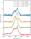 |
Fig. 2. Hα line observed in different years. All observations show the spectra at a similar orbital phase φ ≈ 0.24. All spectra are normalised; the spectra obtained with HARPS and UVES are shown binned to match the resolution of the X-shooter data. A vertical offset was applied to the spectra for clarity. |
The high resolution of the HARPS data allows us to study the emission lines in great detail. To inspect the general spectral energy distribution (SED), however, a larger wavelength range was needed, and we combined archival data from the various instruments mentioned in Sect. 2. The result is displayed in Fig. 3. The SED shows a continuous increase in the flux towards shorter wavelengths; no indication of a maximum from a Planck-curve is present. The spectrum follows a power law with a slope of −2.6. This slope is similar to the slope of a hot steady-state disc, which is expected to be −2.3 (Lynden-Bell 1969). Godon et al. (2017) derived slopes of IUE spectra for a set of 105 CVs including IX Vel, for which they derived value of −2.2, similar to other disc-dominated NLs in the sample. We can therefore conclude that the flux is dominated by the accretion disc, as has been seen in other NL stars when accreting (see e.g. Rodríguez-Gil et al. 2012). This is similar to DW UMa, for example, for which the contribution of the accretion disc to the SED in the UV and the fact that the WD is completely overshone were nicely demonstrated (Knigge et al. 2004).
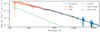 |
Fig. 3. SED of IX Vel obtained with different instruments. The X-shooter and HST spectra are presented in their original flux; the flux of IUE and UVES spectra was multiplied by an arbitrary factor to match the values of the X-shooter and HST spectra. The green line represents the expected contribution of a WD with a temperature of T = 60 000 K, mass MWD = 0.8 M⊙, radius RWD = 0.015 R⊙ (Linnell et al. 2007), and distance d = 90 pc (Gaia Collaboration 2020). The black dashed line represents a fit to the spectrum with a power law whose slope is −2.6. |
4. Radial velocities
The line profile consists of multiple components, each of which we studied separately. This allowed us to probe the radial velocities of the WD with different methods and to also determine the radial velocity curve of the irradiated face of the secondary. Below, we present the analysis of the radial velocities measured from the absorption components, the broad emission components, and the narrow emission components observed in the HARPS data.
4.1. Absorption features
To derive the radial velocities of the absorption components of Hα, Hβ, Hγ, Hδ, and Hε we needed to minimise the influence of the emission lines within the absorption troughs. To achieve this, we opted for a procedure of fitting and cross-correlating in two steps. First, we constructed an average absorption line profile by fitting each line with a Gaussian and determining its average value. This average profile was then used to determine the radial velocities by cross-correlation. The central emission lines were masked during both steps, so the derived value was influenced only by the wings of the absorption line. Figure 4 shows an example of the absorption profile fitting in the case of the Hβ line. When computing the mean values, we treated spectra obtained in 2017 and 2019 separately to accommodate for the mentioned changes in the absorption profile. The cross-correlation of the absorption component of Hα was performed only for the 2019 spectra because it was too weak in the 2017 spectra.
 |
Fig. 4. Sample plot of the Hβ line observed on February 21, 2019 showing the fitting of the absorption line and the absorption-corrected spectra, the observational data are binned for clarity. |
We fitted each radial velocity curve with a sine function defined as

where vrad is the radial velocity, φ0 is the zero point of the ephemeris, γ is the systemic velocity, and K is the velocity amplitude. The parameters of the best fitting models are given in Table 2; Fig. 5 shows the radial velocities obtained in 2019 phased-folded on the orbital period.
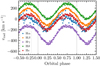 |
Fig. 5. Radial velocity curves of absorption components of Balmer lines observed in the 2019 HARPS spectra. The solid lines show the best fitting models to the radial velocity curves, and the best fitting parameters are given in Table 2. |
Best fitting parameters to the radial velocity curves derived from the analysis of the Balmer lines.
Except for Hα, all velocity curves based on the hydrogen absorption lines have a similar zero phase. Hα is noticeably phase-shifted, as can be seen in Fig. 5. Since Hα has the weakest absorption component out of the hydrogen lines, it is likely that the velocity determination was affected by the contribution of the emission component.
The γ-velocities differ for the separate velocity curves between values ∼ − 500 km s−1 and ∼160 km s−1. The shift of the radial velocity curve is most notable in the case of Hγ, which is significantly blue-shifted with respect to the other hydrogen lines. This is most likely caused by the blending of the hydrogen absorption lines with metal lines present in the spectra, causing an asymmetric line profile around 4300 Å, as can be seen in Fig. 1. The wavelength calibration of the spectra is robust enough for the discrepancies to be caused by calibration inaccuracies.
4.2. Broad emission lines
As an additional check, the wings of the Hα and Hβ emission lines were used to determine radial velocities via the method of fitting a double-Gaussian profile as described by Schneider & Young (1980) and Shafter (1983).
For this analysis, the spectra were corrected for the absorption features (see Sect. 4.1) by re-normalising the spectra to the average absorption profile of the corresponding line. We did not apply this correction to the spectra of the Hα line obtained in 2017 as absorption in these spectra could not be reliably estimated. The width of the Gaussian profiles was set to σ = 1.2 Å for spectra of the Hβ line obtained in 2017 and σ = 2 Å for all other instances. The best value for the separation of the two Gaussians was determined from the diagnostic diagrams as the separation, for which the relative error of the semi-amplitude  has the smallest value. In the case of Hβ the separation was a = 10.0 Å for the 2017 spectra and a = 10.67 Å for the 2019 data; in the case of Hα the separation was a = 7.29 Å for the 2017 spectra and a = 10.18 Å for the 2019 data. The diagnostic diagram for Hα line based on the 2019 data is shown in Fig. 6. The separation of the two Gaussians should correspond to the same shift in radial velocity for each line; however, this is not the case for Hα and Hβ. The ideal separation for Hβ is larger than for Hα, contrary to the expectation. This is likely caused by the presence of the absorption component. The presence of the absorption component, which could not be corrected in the case of the 2017 data, results in a smaller separation a compared to that of Hβ. Even though the 2019 data of Hα were corrected for absorption, its profile could have been determined inaccurately due to its low prominence.
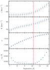 |
Fig. 6. Diagnostic diagram for the Hα emission line based on 2019 observations. The red dashed line marks the separation a = 11.16 Å, which was used for the radial velocity determination. |
Figure 7 shows the radial velocities based on the wings of Hα and Hβ observed in 2019 and compares them with the radial velocities determined from the absorption component. The parameters of the best fits of the derived radial velocity curves are listed in Table 2. There is a clear phase offset between the radial velocity curves obtained from the broad emission lines and those obtained from the absorption lines.
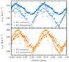 |
Fig. 7. Radial velocity curves based on the broad emission component of Hα and Hβ emission lines observed in 2019. Radial velocities derived from the absorption component are plotted for comparison. |
This is a known problem of determining radial velocity from the broad emission lines (see Warner 1995, Chap. 2.7.6) which is caused by asymmetric brightness distribution. While these usually originate in the accretion disc, bright emission line regions outside the disc, as discussed above, would have the same effect. While the double-Gaussian method combined with the diagnostic diagram takes care of the typical asymmetric effects coming from the bright spot at the outer rim of the accretion disc, any asymmetry at higher velocities, whether originating from inside the disc or from material further outside bound to the binary orbit, will cause a phase shift in the radial velocities derived from the wings of the emission lines. It should also be kept in mind that while emission from the inner part of the disc could contribute to the wings of the broad emission line, the absorption component is observed even further outside at higher radial velocities, and therefore offers a more robust way to analyse the inner part of the disc. Because of these discussed limitations of the diagnostic diagram method, we decided to use the radial velocity curves derived from the strong absorption components in the subsequent analysis.
4.3. Narrow emission line
Radial velocities of the narrow emission component of the Hα line were determined by fitting the spectra with a multi-component model consisting of four Gaussians: one to fit the absorption component, one to fit the narrow emission, and two to fit the remaining emission originating in the disc. The radial velocities were then computed from the position of the Gaussian representing the narrow emission. The resulting radial velocity curve is plotted in Fig. 8. We observed no significant difference between the radial velocity curves obtained from 2017 and 2019 observations, and therefore we fitted all the HARPS data simultaneously with a sine function. The parameters of the best fit are given in Table 2.
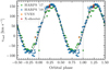 |
Fig. 8. Radial velocity of narrow component of Hα based on HARPS, UVES, and X-shooter data. The dashed line represents the best fit to the presented data. |
The semi-amplitude determined by the fitting is in good agreement with the value presented by Beuermann & Thomas (1990), and our radial velocity curve is anti-phased to those derived from absorption lines and broad emission lines as also found by those authors, who concluded that the narrow emission originates from the irradiated side of the secondary star. The radial velocity curve of the narrow component is in agreement with the velocity values derived from the narrow component using the X-shooter and UVES spectra, as can be seen in Fig. 8.
4.4. O–C diagram
We used all the Balmer absorption lines except for Hα to determine the moments of the zeroth phase for each night. This was achieved by simultaneously fitting the radial velocity curve with the zeroth phase being a shared free parameter for all curves. The derived moments of the zeroth phase are listed in Table 3 together with previously published data. As the error of the orbital period determined by Kubiak et al. (1999) is 4 × 10⁻⁷ d and the time elapsed between observations of Kubiak et al. (1999) and HARPS observations corresponds to ∼50 000 epochs, the zeroth phase for the HARPS observations could be predicted with an accuracy of ∼0.1 in the orbital phase. This accuracy was high enough to reliably determine the epoch numbers of the HARPS observations. We used the data presented in Table 3 to derive an improved spectroscopic ephemeris of the system:

Moments of spectroscopic phase zero.
The O−C diagram of the moments of phase zero constructed with the improved spectroscopic ephemeris is shown in Fig. 9.
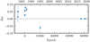 |
Fig. 9. O−C diagram for times of the zeroth phase derived from the radial velocity curves. |
The times of zeroth phases presented in Table 3 were determined from radial velocities obtained with different methods. Radial velocities published by Wargau et al. (1983) and Eggen & Niemela (1984) were calculated from the central positions of the Balmer hydrogen lines. Beuermann & Thomas (1990) used a two-component model consisting of two Gaussians to model the emission in Hα and Hβ, where one component (sharp) represented the emission originating from the secondary, and one component (broad) represented the emission originating in the disc. Beuermann & Thomas (1990) then used the radial velocities of the broad component to determine the times of the zeroth phase. Kubiak et al. (1999) used emission lines of hydrogen and Ca II observed in the spectral range between 8090 Å and 9200 Å to determine the velocities by fitting each line with a Gaussian.
The different approaches used to determine the zeroth phase might cause scatter in the O−C diagram, which would not reflect real physical changes caused by the dynamics of the system; similarly, we see a phase offset between the radial velocity curves of absorption and emission discussed in Sect. 4.2.
5. Doppler tomography
We used Doppler tomography to map the accretion disc in velocity coordinates (vx, vy). This technique was developed by Marsh & Horne (1988) and uses time-resolved spectroscopic observations to compute maps of the system that display the intensity of the emission line emitted at velocity coordinates (vx, vy). We employed the code by Spruit (1998), which applies the maximum entropy method to compute the Doppler maps. We used the PYTHON3 programming language to plot the maps. The Roche lobe, stream, and position of the components overlaid on the maps were plotted using the PYTHON3 package PYDOPPLER4 by Hernandez Santisteban (2021). When plotting the Roche lobe and the accretion stream, we assumed the mass of the primary MWD = 0.8 M⊙ and the mass of the secondary M2 = 0.52 M⊙, which were derived by Linnell et al. (2007). This gives the mass ratio q = 0.65.
We binned the spectra used for the computation by a factor of 30, which filtered out the noise present in the spectra, but still provided a spectral resolution high enough to study the structure of the system. We combined all HARPS spectra when computing the maps, as maps computed for individual nights did not show any significant changes in the structure, which was also the case for the individual spectra, as can be seen in Fig. 2. The orbital phases of the spectra were computed using Eq. (2), which proved to be precise enough to combine data obtained two years apart. We computed maps for the emission lines with sufficient signal-to-noise ratio; all the Doppler maps are presented in Fig. 10, and the same maps but in inverse hyperbolic sine scale are shown in Fig. A.1. The spectra of the Hα line were contaminated by telluric lines and the spectra of Hε were contaminated by interstellar lines, which would create fake circular structures in the Doppler maps of these lines. We therefore corrected the spectra for the contamination by normalising them to an average spectrum of contaminating lines, and the Doppler maps presented are free of these fake structures.
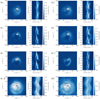 |
Fig. 10. Doppler tomography based on HARPS observations from all three nights. The colour of the Doppler maps corresponds to arbitrary units of emission intensity. The positions of the primary and secondary are given by plus signs, the centre of mass by the cross, and the position of the L3 point by the star. The velocity of the L3 point corresponds to its velocity caused by the rotation of the binary system; the Keplerian velocity of the disc extrapolated to this location is greater by about 40 km s−1. Roche lobes of both components and the expected stream trajectory are outlined by solid lines, the tidal limitation radius is outlined by the dashed circle. The Doppler maps were computed from lines Hα, Hβ, Hγ, Hδ, Hε, He Iλ6677 Å, He IIλ4686 Å and from the Bowen blend (BB). All maps derived from the analysis of the Balmer lines are corrected for the presence of the absorption features, as described in Sect. 4.1. For each map a trailed spectrum of the corresponding line is shown. The scale of the Doppler maps was chosen to highlight the observed structures and does not correspond to the scale of trailed spectra. Figure A.1 shows the same Doppler maps, only in inverse hyperbolic sine scale, in which the low-amplitude features are highlighted. |
The Doppler maps of the hydrogen and He Iλ6677 Å lines show a bright emission corresponding to the velocity coordinates of the part of the secondary adjacent to the Lagrangian L1 point. This emission is also the dominant feature in the trailed spectra of these lines with maximum brightness around phase φ = 0.5, which corresponds to the face-on view of the irradiated part of the secondary. In spectra obtained close to phase φ = 0.0, when the irradiated part of the secondary is hidden out-of-view, we see little to no emission originating from that region; however, in some cases (e.g. the Hα line) it does not disappear completely.
Doppler maps of Hα, Hβ, and He Iλ6677 Å show an arm-like feature in the lower-right quadrant (vx = 200 km s−1, vy = −250 km s−1), which is located outside of the tidal-limitation radius. This feature corresponds to the position of an outflow from the accretion disc in the work by Bisikalo & Kononov (2010). This outflow gives rise to a gaseous circumbinary envelope, and the model by Bisikalo & Kononov (2010) shows the presence in a region outside the disc of matter connecting to a bow shock, which forms as the binary moves through the circumbinary envelope. The emission from this outflow region, as computed by Bisikalo & Kononov (2010), is located in our Doppler maps at coordinates of vx ≳ 0 km s−1 outside of the accretion disc. Similar structures have been observed in other NLs, for example RW Sex, 1RXS J064434.5+334451 (Hernandez et al. 2017), and RW Tri (Subebekova et al. 2020).
The Doppler maps of the Balmer lines show an emission region that coincides with the position of the tidal-limitation radius, even though in the case of Hα and Hβ it is less prominent when compared with other features in those maps. We interpret this feature as the emission from the outer rim of the accretion disc. It does not have the usual doughnut shape, which is typical for accretion discs of CVs as the emission intensity is not circularly symmetric with the lower part exhibiting weaker emission. This could be caused by matter in the outflow region blocking the view of the accretion disc.
Doppler maps of He IIλ4686 and the Bowen blend show the highest intensity at low velocities outside of the accretion disc; the map of He II has the highest intensity at coordinates (vx ∼ −200 km s−1, vy ∼ −50 km s−1) and the maximum intensity in the map of the Bowen blend is centred on the centre of mass of the system. The low velocities suggest that these lines are formed in wind from the accretion disc. This is similar to the NL SW Sex, which also shows low-velocity emission in He IIλ4686 and the Bowen blend, which Honeycutt et al. (1986) interpreted as wind emission. Similarly, observations of DN IP Peg in outburst presented by Marsh & Horne (1990) show a low-velocity He IIλ4686 emission, and its Doppler maps has maximum intensity at a similar position to that of IX Vel.
6. Doppler map of near-infrared emission lines
Kubiak et al. (1999) analysed time-resolved near-infrared spectra and fitted the observed spectral lines with a three-component model. Even though they did not present a Doppler map based on their time-resolved spectra, their three-component model allowed us to reconstruct a Doppler map of IX Vel. We used the parameters presented by Kubiak et al. (1999) in their Table 4 and the relative strengths of Ca IIλ8542 given in their Table 3 to compute a set of phase-resolved spectra. We subtracted a value of 0.13 from the phase parameter of each component so that the parameter Φ2 = 0 and the zeroth phase was the moment of the inferior conjunction of the secondary. We then used the spectra to compute a Doppler map; the resulting map is presented in Fig. 11.
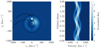 |
Fig. 11. Doppler map (left) and trailed spectra (right) based on the three-component model of emission lines presented by Kubiak et al. (1999). |
The map shows that the components, which Kubiak et al. (1999) call the disc component and the hot spot component, lie outside of the tidal limitation radius of the accretion disc, and that the hot spot component is not located in the usual position of the bright spot. Therefore, the two components are more likely linked to an outflow material from the system. All the emission from the model originates at velocities lower than 500 km s−1, which resembles several maps presented in Fig. 10, especially the map of Hα where most of the emission can be found at lower velocities. The hot spot component of Kubiak’s model is located at coordinates (vx = 200 km s−1, vy = −50 km s−1) and coincides with an emission source found in our Doppler maps, most noticeably in the map of Hγ.
7. Temperature distribution map
We obtained Doppler maps of five Balmer lines that show the intensity of the corresponding line in velocity coordinates. This intensity is dependent on the hydrogen density in the disc and on the temperature of hydrogen, but a Doppler map based on a single line is not sufficient to distinguish between temperature-related structures and density-related structures. We used the Doppler maps to compute an approximate temperature distribution map following a method that was used by Rutkowski et al. (2016) to compute a temperature distribution map of the accretion disc of the dwarf nova V2051 Oph. This method uses the assumption that the spectrum emitted by the accretion disc can be modelled by an isothermal and isobaric pure-hydrogen slab whose flux can be described by a function
where Bλ(T) is the Planck function describing the black-body radiation and τλ is the wavelength dependant optical depth. The method further assumes that the optical depth in emission lines is centred at τλ > 1 and is significantly higher than in the continuum. Under this assumption, the decrements of the Balmer lines should be described by a Planck function and the temperature of an element with coordinates (vx, vy) can be estimated by fitting the flux values of corresponding elements of different Doppler maps with a black body.
We used the Doppler maps of the Hα, Hβ, Hδ, and Hε emission lines to construct a map of the temperature distribution for the disc in IX Vel. We excluded the map of the Hγ emission line because the absorption component of this line was too complex to be sufficiently fitted by a single Gaussian, probably due to blending with metal lines in its vicinity. As a result, the Doppler map based on the reconstructed emission component could represent incorrect flux values unsuitable for the estimation of the temperature distribution.
The Doppler maps presented in Fig. 10 were produced from normalised spectra, and therefore for the temperature map computation we scaled each map by the flux of the continuum at the position of each corresponding line. The scaling factors were derived by fitting the flux-calibrated X-shooter spectra of IX Vel with a Planck function.
We decided to compute the temperature distribution map for a grid with pixels of a larger size than those of the Doppler maps in order to minimise the effect of noise in the Doppler maps affecting the temperature distribution values. Averaging over a larger area is important, especially for such (vx, vy) where the intensity of the emission lines is low. As can be seen on the Doppler maps in Fig. 10, low-intensity regions are located predominantly at high velocities. We therefore decided to use a polar grid for the temperature distribution map with its centre located at the position of the WD. With this set-up, the temperature for higher velocities is based on more pixels of the Cartesian grid and the symmetry of the polar grid reflects the shape of a circular accretion disc with its centre at the WD position. We also excluded pixels with high-velocity coordinates, which did not contain enough signal for a reliable fit, and we computed the temperature distribution map only for a circular mask with a radius of v = 750 km s−1 centred on the WD. The mask was divided into 60 annuli and 30 sectors.
The resulting temperature distribution map is shown in Fig. 12 together with a map showing the corresponding errors. The map itself should be considered only a rough approximation of the actual temperature distribution, as numerous assumptions about the origin of the emission lines were used. For this reason, we also do not interpret the temperature values as absolute, but rather as relative values used to distinguish various features in the system.
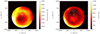 |
Fig. 12. Temperature map based on Doppler maps of lines Hα, Hβ, Hδ, Hε (left panel) and the estimated error of the temperature map (right panel). |
The area of the map with the highest temperature (T > 8500 K) is located at the high velocities in the lower left quadrant (vx = −600 km s−1, vy = −400 km s−1) and extends to the bottom part of the map. This area, however, also has the largest error estimates, and therefore its existence is dubious. Another region of high temperature (T ≃ 7500 K) is in the upper left quadrant corresponding to the expected position of a bright spot. Similarly to the Doppler maps, structures corresponding to the tidal-limitation radius are present, but are not circularly symmetrical, with the rim of the disc in the lower left quadrant being colder than the rest of the disc. The temperature along the tidal limitation radius varies between T ≃ 6300 K and T ≃ 7200 K with an average temperature of about T ≃ 6900 K. The irradiated face of the secondary is also present in the temperature distribution map (T ≃ 6700 K), although it is a less prominent feature than in the Doppler maps presented in Fig. 10. Even if the absolute values are not to be trusted, we can say that in relation to each other, the bright spot area is about 600 K hotter than its surroundings. This is consistent with the findings of Linnell et al. (2007), that the bright spot can be only about 500 K hotter than the rest of the rim of the disc.
8. IX Vel as an RW Sex star
The Doppler maps of IX Vel resemble the maps of RW Sex and 1RXS J064434.5+334451 constructed by Hernandez et al. (2017). Both systems are NL stars and exhibit strong emission from the illuminated face of the secondary and additional emission corresponding to the position of an outflow zone. Similar features are also observed in RW Tri (Subebekova et al. 2020) and BG Tri (Hernández et al. 2021), which prompted Hernandez to group them together, with RW Sex as the prototype. IX Vel fits well within these systems and can be considered as belonging to the group of RW Sex stars as defined by Hernandez et al. (2017).
However, many other NLs show one or the other of these features: Thoroughgood et al. (2004) presented Doppler tomography of AC Cnc and V363 Aur, both of which show emission from the secondary close to the L1 point and low-velocity emission, which appears to originate outside of the accretion disc. In the case of AC Cnc, the low-velocity emission is circularly symmetrical and could also be related to a wind originating in the disc. For V363 Aur, the low-velocity emission is located at negative vy velocities and strongly resembles emission from an outflow zone described in the previously mentioned systems. Low-velocity emission that seems to originate outside of the accretion disc can be also found in the Doppler maps of the Balmer lines of SW Sex and DW UMa constructed by Dhillon et al. (2013), even though in the case of SW Sex the emission lies close to the tidal limitation radius and could therefore originate in the disc as well. These two systems do not show emission originating at the secondary, but they show emission linked to the bright spot and in the case of SW Sex also emission linked to the gas stream. Dhillon et al. (2013) also constructed Doppler maps for He II for both SW Sex and DW Uma. While their He II map of SW Sex looks similar to the maps of the Balmer lines, the map of DW UMa shows emission centred on the WD which likely originates in an accretion disc wind. The latter was also recently reported in system ASAS J071404+7004.3 by Inight et al. (2022). This raises the question of whether all these stars are potential members of the RW-Sex group. It seems that many of these systems also belong to the SW Sex stars or are at least NLs with high mass-transfer rates. The presence of an outflow as well as the strong irradiation of the secondary might be expected for such systems, and would thus be another indication for a high mass-transfer system. SW Sex stars show a strong emission originating in the bright spot and an absorption feature near the orbital phase φ = 0.5, which Tovmassian et al. (2014) interprets as evidence of the outflow zone. In the case of long-period NLs (Porb > 4 h), the outflow region is observed as a strong emission source and the bright spot is not a prominent feature in these systems (Hernandez et al. 2017).
The presence of outflows in NLs plays an important role in understanding the evolution of CVs as it would provide an additional mechanism for orbital angular momentum loss, acting alongside the traditionally considered magnetic braking and gravitational wave radiation. Schmidtobreick (2013) finds that almost all CVs with orbital periods in the range between 2.8 h and 4 h are NLs of SW Sex type, and concludes that they must represent an evolutionary phase of CVs as all long-period CVs will eventually travel through this period range. The few systems in this period range for which the secular mass-transfer was measured (see Pala et al. 2017, and references therein) show high accretion rates, much higher than predicted from the models (Knigge et al. 2011). This indicates that additional braking mechanisms are indeed needed to explain these systems, and several have been discussed in the literature (Zangrilli et al. 1997; Townsley & Gänsicke 2009; Knigge et al. 2011). The presence of outflows as observed in IX Vel and the above-mentioned systems (see Table 4) could be another option.
Examples of single-peaked NLs with similar characteristics to IX Vel
9. Conclusion
We analysed the time-resolved spectroscopy of IX Vel that was obtained during two different runs, one in 2017 and one in 2019. While the general structure of the spectra was the same during both runs, a comparison with spectra obtained on other occasions showed that it is not a general rule for this system. Namely, the hydrogen emission line profiles observed in 2017 and 2019 significantly vary from those obtained few years before, in 2014.
We used time-resolved spectroscopy to determine the radial velocity curves of several features of spectral lines and to improve the spectroscopic ephemeris of the system.
We constructed Doppler maps of the system using the emission lines of hydrogen, helium, and the Bowen blend. The maps of hydrogen and He I show a strong emission originating from the irradiated surface of the secondary, emission from the outer part of the accretion disc and emission originating outside of the disc, which we interpret as a possible outflow from the disc. Maps of He II and the Bowen blend show emission at low velocities, which we interpret as emission from the accretion disc winds. We conclude that IX Vel can be considered a member of the RW Sex stars as defined by Hernandez et al. (2017). Although some maps show a hint of a bright spot emission, most notably the map of He I, there is no strong emission originating from its position.
We used the Doppler maps of Hα, Hβ, Hδ, and Hε to compute a temperature distribution map of the system. Due to the strong assumptions used for the computation, the resulting map should only be viewed as a relative temperature distribution in the system. The map shows high-temperature features that can be interpreted as the bright spot of the accretion disc, the rim of the accretion disc, and the irradiated face of the secondary. In agreement with Linnell et al. (2007), we find temperatures of the bright spot to be about 600 K brighter than the rest of the accretion disc rim.
The emission originating in the outflow zone, which we see in the Doppler maps of IX Vel, was also observed in other NLs that show signs of high mass-transfer. As the velocities corresponding to the outflow zone are low, its structure in the Doppler maps can only be probed using high-resolution time-resolved spectra. To further study the plenitude of such outflows, Doppler tomography of the known high mass-transfer NL systems based on high-resolution spectra are needed to resolve the structure of these low-velocity components in the emission lines and to establish a census of their occurrence.
Kubiak et al. (1999) give a value for the transit φ = 0.32; however, it is not corrected for the phase offset of the spectra, which can be determined from the phase offset of the radial velocity curves of the secondary and the disc. Here we present the corrected value. In both cases, however, the position of the hot spot component does not match the position of a typical CV bright spot.
Available at https://archive.eso.org/cms.html
Available at https://sky.esa.int/esasky/
Available at github.com/Alymantara/pydoppler
Acknowledgments
We are grateful to the anonymous referee for providing us with useful comments and suggestions that improved our manuscript. We thank Marek Wolf for useful discussions and comments. Based on observations collected at the European Organisation for Astronomical Research in the Southern Hemisphere under ESO programmes 60.A-9700, 094.D-0344, 69.C-0171 and 088.D-0537. Based on data obtained from the ESO Science Archive Facility with DOIs: https://doi.org/10.18727/archive/33, https://doi.org/10.18727/archive/50, https://doi.org/10.18727/archive/71. This research has made use of ESASky, developed by the ESAC Science Data Centre (ESDC) team and maintained alongside other ESA science mission’s archives at ESA’s European Space Astronomy Centre (ESAC, Madrid, Spain). This research is based on observations made with the NASA/ESA Hubble Space Telescope obtained from the Space Telescope Science Institute, which is operated by the Association of Universities for Research in Astronomy, Inc., under NASA contract NAS 5-26555. These observations are associated with program 14637. This research was supported by the Ministry of Education, Youth and Sports (Czech Republic).
References
- Baines, D., Giordano, F., Racero, E., et al. 2017, PASP, 129, 028001 [NASA ADS] [CrossRef] [Google Scholar]
- Beuermann, K., & Thomas, H. C. 1987, Mitteilungen der Astronomischen Gesellschaft Hamburg, 70, 369 [Google Scholar]
- Beuermann, K., & Thomas, H. C. 1990, A&A, 230, 326 [NASA ADS] [Google Scholar]
- Bisikalo, D. V., & Kononov, D. A. 2010, Mem. Soc. Astron. It., 81, 187 [Google Scholar]
- Boggess, A., Bohlin, R. C., Evans, D. C., et al. 1978a, Nature, 275, 377 [NASA ADS] [CrossRef] [Google Scholar]
- Boggess, A., Carr, F. A., Evans, D. C., et al. 1978b, Nature, 275, 372 [NASA ADS] [CrossRef] [Google Scholar]
- Cordova, F. A., & Mason, K. O. 1982, ApJ, 260, 716 [NASA ADS] [CrossRef] [Google Scholar]
- Dekker, H., D’Odorico, S., Kaufer, A., Delabre, B., & Kotzlowski, H. 2000, SPIE Conf. Ser., 4008, 534 [Google Scholar]
- Dhillon, V. S., Marsh, T. R., & Jones, D. H. P. 1997, MNRAS, 291, 694 [Google Scholar]
- Dhillon, V. S., Smith, D. A., & Marsh, T. R. 2013, MNRAS, 428, 3559 [Google Scholar]
- Eggen, O. J., & Niemela, V. S. 1984, AJ, 89, 389 [CrossRef] [Google Scholar]
- Freudling, W., Romaniello, M., Bramich, D. M., et al. 2013, A&A, 559, A96 [NASA ADS] [CrossRef] [EDP Sciences] [Google Scholar]
- Gaia Collaboration 2020, VizieR Online Data Catalog: I/350 [Google Scholar]
- Garrison, R. F., Hiltner, W. A., & Schild, R. E. 1982, IAU Circ., 3730, 2 [NASA ADS] [Google Scholar]
- Garrison, R. F., Schild, R. E., Hiltner, W. A., & Krzeminski, W. 1984, ApJ, 276, L13 [NASA ADS] [CrossRef] [Google Scholar]
- Giordano, F., Racero, E., Norman, H., et al. 2018, Astron. Comput., 24, 97 [NASA ADS] [CrossRef] [Google Scholar]
- Godon, P., Sion, E. M., Balman, Ş., & Blair, W. P. 2017, ApJ, 846, 52 [NASA ADS] [CrossRef] [Google Scholar]
- Haug, K. 1988, MNRAS, 235, 1385 [Google Scholar]
- Hernandez Santisteban, J. V. 2021, Astrophysics Source Code Library [record ascl:2106.003] [Google Scholar]
- Hernandez, M. S., Zharikov, S., Neustroev, V., & Tovmassian, G. 2017, MNRAS, 470, 1960 [NASA ADS] [CrossRef] [Google Scholar]
- Hernández, M. S., Tovmassian, G., Zharikov, S., et al. 2021, MNRAS, 503, 1431 [Google Scholar]
- Honeycutt, R. K., Schlegel, E. M., & Kaitchuck, R. H. 1986, ApJ, 302, 388 [NASA ADS] [CrossRef] [Google Scholar]
- Inight, K., Gänsicke, B. T., Blondel, D., et al. 2022, MNRAS, 510, 3605 [NASA ADS] [CrossRef] [Google Scholar]
- Kato, T. 2021, arXiv e-prints [arXiv:2111.15145] [Google Scholar]
- Kausch, W., Noll, S., Smette, A., et al. 2015, A&A, 576, A78 [NASA ADS] [CrossRef] [EDP Sciences] [Google Scholar]
- Knigge, C., Araujo-Betancor, S., Gänsicke, B. T., et al. 2004, ApJ, 615, L129 [NASA ADS] [CrossRef] [Google Scholar]
- Knigge, C., Baraffe, I., & Patterson, J. 2011, ApJS, 194, 28 [Google Scholar]
- Kochanek, C. S., Shappee, B. J., Stanek, K. Z., et al. 2017, PASP, 129, 104502 [Google Scholar]
- Kubiak, M., Pojmanski, G., & Krzeminski, W. 1999, Acta Astron., 49, 73 [NASA ADS] [Google Scholar]
- Linnell, A. P., Godon, P., Hubeny, I., Sion, E. M., & Szkody, P. 2007, ApJ, 662, 1204 [NASA ADS] [CrossRef] [Google Scholar]
- Lynden-Bell, D. 1969, Nature, 223, 690 [NASA ADS] [CrossRef] [Google Scholar]
- Marsh, T. R., & Horne, K. 1988, MNRAS, 235, 269 [Google Scholar]
- Marsh, T. R., & Horne, K. 1990, ApJ, 349, 593 [NASA ADS] [CrossRef] [Google Scholar]
- Matthews, J. H., Knigge, C., Long, K. S., Sim, S. A., & Higginbottom, N. 2015, MNRAS, 450, 3331 [NASA ADS] [CrossRef] [Google Scholar]
- Mauche, C. W. 1991, ApJ, 373, 624 [NASA ADS] [CrossRef] [Google Scholar]
- Mayor, M., Pepe, F., Queloz, D., et al. 2003, The Messenger, 114, 20 [NASA ADS] [Google Scholar]
- Pala, A. F., Gänsicke, B. T., Townsley, D., et al. 2017, MNRAS, 466, 2855 [NASA ADS] [CrossRef] [Google Scholar]
- Pojmanski, G. 1997, Acta Astron., 47, 467 [Google Scholar]
- Rodríguez-Gil, P., Schmidtobreick, L., Long, K. S., et al. 2012, MNRAS, 422, 2332 [Google Scholar]
- Rutkowski, A., Waniak, W., Preston, G., & Pych, W. 2016, MNRAS, 463, 3290 [Google Scholar]
- Schmidtobreick, L. 2013, Cent. Eur. Astrophys. Bull., 37, 361 [Google Scholar]
- Schneider, D. P., & Young, P. 1980, ApJ, 238, 946 [NASA ADS] [CrossRef] [Google Scholar]
- Shafter, A. W. 1983, ApJ, 267, 222 [NASA ADS] [CrossRef] [Google Scholar]
- Shappee, B. J., Prieto, J. L., Grupe, D., et al. 2014, ApJ, 788, 48 [Google Scholar]
- Sion, E. M. 1985, ApJ, 292, 601 [NASA ADS] [CrossRef] [Google Scholar]
- Smette, A., Sana, H., Noll, S., et al. 2015, A&A, 576, A77 [NASA ADS] [CrossRef] [EDP Sciences] [Google Scholar]
- Spruit, H. C. 1998, arXiv e-prints [arXiv:astro-ph/9806141] [Google Scholar]
- Subebekova, G., Zharikov, S., Tovmassian, G., et al. 2020, MNRAS, 497, 1475 [Google Scholar]
- Thoroughgood, T. D., Dhillon, V. S., Watson, C. A., et al. 2004, MNRAS, 353, 1135 [Google Scholar]
- Tovmassian, G., Stephania Hernandez, M., González-Buitrago, D., Zharikov, S., & García-Díaz, M. T. 2014, AJ, 147, 68 [Google Scholar]
- Townsley, D. M., & Gänsicke, B. T. 2009, ApJ, 693, 1007 [Google Scholar]
- Vernet, J., Dekker, H., D’Odorico, et al. 2011, A&A, 536, A105 [NASA ADS] [CrossRef] [EDP Sciences] [Google Scholar]
- Wargau, W., Drechsel, H., Rahe, J., & Bruch, A. 1983, MNRAS, 204, 35P [NASA ADS] [CrossRef] [Google Scholar]
- Wargau, W., Bruch, A., Drechsel, H., Rahe, J., & Schoembs, R. 1984, Ap&SS, 99, 145 [NASA ADS] [CrossRef] [Google Scholar]
- Warner, B. 1995, Camb. Astrophys. Ser., 28 [Google Scholar]
- Warner, B., Odonoghue, D., & Allen, S. 1985, MNRAS, 212, 9P [Google Scholar]
- Williams, G. A., & Hiltner, W. A. 1984, MNRAS, 211, 629 [Google Scholar]
- Woods, A. J., Drew, J. E., & Verbunt, F. 1990, MNRAS, 245, 323 [Google Scholar]
- Zangrilli, L., Tout, C. A., & Bianchini, A. 1997, MNRAS, 289, 59 [NASA ADS] [Google Scholar]
Appendix A: Doppler maps in inverse hyperbolic sine scale
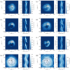 |
Fig. A.1. Same as Fig. 10, but the Doppler maps are shown in inverse hyperbolic sine scale to highlight low-amplitude features. |
All Tables
Best fitting parameters to the radial velocity curves derived from the analysis of the Balmer lines.
All Figures
|
Fig. 1. Average spectra of IX Vel obtained with HARPS on January 11, 2017, and on February 20, 2019. The 2017 spectrum is vertically shifted for clarity. The spectrum has been corrected for telluric lines. The main emission and absorption features are labelled. |
| In the text | |
|
Fig. 2. Hα line observed in different years. All observations show the spectra at a similar orbital phase φ ≈ 0.24. All spectra are normalised; the spectra obtained with HARPS and UVES are shown binned to match the resolution of the X-shooter data. A vertical offset was applied to the spectra for clarity. |
| In the text | |
|
Fig. 3. SED of IX Vel obtained with different instruments. The X-shooter and HST spectra are presented in their original flux; the flux of IUE and UVES spectra was multiplied by an arbitrary factor to match the values of the X-shooter and HST spectra. The green line represents the expected contribution of a WD with a temperature of T = 60 000 K, mass MWD = 0.8 M⊙, radius RWD = 0.015 R⊙ (Linnell et al. 2007), and distance d = 90 pc (Gaia Collaboration 2020). The black dashed line represents a fit to the spectrum with a power law whose slope is −2.6. |
| In the text | |
|
Fig. 4. Sample plot of the Hβ line observed on February 21, 2019 showing the fitting of the absorption line and the absorption-corrected spectra, the observational data are binned for clarity. |
| In the text | |
|
Fig. 5. Radial velocity curves of absorption components of Balmer lines observed in the 2019 HARPS spectra. The solid lines show the best fitting models to the radial velocity curves, and the best fitting parameters are given in Table 2. |
| In the text | |
|
Fig. 6. Diagnostic diagram for the Hα emission line based on 2019 observations. The red dashed line marks the separation a = 11.16 Å, which was used for the radial velocity determination. |
| In the text | |
|
Fig. 7. Radial velocity curves based on the broad emission component of Hα and Hβ emission lines observed in 2019. Radial velocities derived from the absorption component are plotted for comparison. |
| In the text | |
|
Fig. 8. Radial velocity of narrow component of Hα based on HARPS, UVES, and X-shooter data. The dashed line represents the best fit to the presented data. |
| In the text | |
|
Fig. 9. O−C diagram for times of the zeroth phase derived from the radial velocity curves. |
| In the text | |
|
Fig. 10. Doppler tomography based on HARPS observations from all three nights. The colour of the Doppler maps corresponds to arbitrary units of emission intensity. The positions of the primary and secondary are given by plus signs, the centre of mass by the cross, and the position of the L3 point by the star. The velocity of the L3 point corresponds to its velocity caused by the rotation of the binary system; the Keplerian velocity of the disc extrapolated to this location is greater by about 40 km s−1. Roche lobes of both components and the expected stream trajectory are outlined by solid lines, the tidal limitation radius is outlined by the dashed circle. The Doppler maps were computed from lines Hα, Hβ, Hγ, Hδ, Hε, He Iλ6677 Å, He IIλ4686 Å and from the Bowen blend (BB). All maps derived from the analysis of the Balmer lines are corrected for the presence of the absorption features, as described in Sect. 4.1. For each map a trailed spectrum of the corresponding line is shown. The scale of the Doppler maps was chosen to highlight the observed structures and does not correspond to the scale of trailed spectra. Figure A.1 shows the same Doppler maps, only in inverse hyperbolic sine scale, in which the low-amplitude features are highlighted. |
| In the text | |
|
Fig. 11. Doppler map (left) and trailed spectra (right) based on the three-component model of emission lines presented by Kubiak et al. (1999). |
| In the text | |
|
Fig. 12. Temperature map based on Doppler maps of lines Hα, Hβ, Hδ, Hε (left panel) and the estimated error of the temperature map (right panel). |
| In the text | |
|
Fig. A.1. Same as Fig. 10, but the Doppler maps are shown in inverse hyperbolic sine scale to highlight low-amplitude features. |
| In the text | |
Current usage metrics show cumulative count of Article Views (full-text article views including HTML views, PDF and ePub downloads, according to the available data) and Abstracts Views on Vision4Press platform.
Data correspond to usage on the plateform after 2015. The current usage metrics is available 48-96 hours after online publication and is updated daily on week days.
Initial download of the metrics may take a while.