| Issue |
A&A
Volume 678, October 2023
|
|
|---|---|---|
| Article Number | A134 | |
| Number of page(s) | 11 | |
| Section | Numerical methods and codes | |
| DOI | https://doi.org/10.1051/0004-6361/202245601 | |
| Published online | 17 October 2023 | |
Measuring the numerical viscosity in simulations of protoplanetary disks in Cartesian grids
The viscously spreading ring revisited
1
Institut für Astronomie und Astrophysik, Universität Tübingen,
Auf der Morgenstelle 10,
72076
Tübingen, Germany
2
Astronomy Unit, Department of Physics and Astronomy, Queen Mary University of London,
London
E1 4NS, UK
e-mail: This email address is being protected from spambots. You need JavaScript enabled to view it.
; This email address is being protected from spambots. You need JavaScript enabled to view it.
3
Leibniz-Institut für Astrophysik Potsdam (AIP),
An der Sternwarte 16,
14482
Potsdam, Germany
e-mail: This email address is being protected from spambots. You need JavaScript enabled to view it.
Received:
1
December
2022
Accepted:
24
July
2023
Abstract
Context. Hydrodynamical simulations solve the governing equations on a discrete grid of space and time. This discretization causes numerical diffusion similar to a physical viscous diffusion, the magnitude of which is often unknown or poorly constrained. With the current trend of simulating accretion disks with no or very low prescribed physical viscosity, it has become essential to understand and quantify this inherent numerical diffusion in the form of a numerical viscosity.
Aims. We study the behavior of the viscous spreading ring and the spiral instability that develops in it. We aim to use this setup to quantify the numerical viscosity in Cartesian grids and study its properties.
Methods. We simulated the viscous spreading ring and the related instability on a two-dimensional polar grid using PLUTO as well as FARGO, ensuring the convergence of our results with a resolution study. We then repeated our models on a Cartesian grid and measured the numerical viscosity by comparing results to the known analytical solution using PLUTO and Athena++.
Results. We find that the numerical viscosity in a Cartesian grid scales with resolution as approximately vnum ∝ Δx2 and is equivalent to an effective α ~ 10−4 for a common numerical setup. We also showed that the spiral instability manifests as a single leading spiral throughout the whole domain on polar grids. This is contrary to previous results and indicates that sufficient resolution is necessary in order to correctly resolve the instability.
Conclusions. Our results are relevant in the context of models where the origin should be included in the computational domain, or when polar grids cannot be used. Examples of such cases include models of disk accretion onto a central binary and, inherently, Cartesian codes.
Key words: hydrodynamics / accretion, accretion disks / protoplanetary disks / methods: numerical
© The Authors 2023
 Open Access article, published by EDP Sciences, under the terms of the Creative Commons Attribution License (https://creativecommons.org/licenses/by/4.0), which permits unrestricted use, distribution, and reproduction in any medium, provided the original work is properly cited.
This article is published in open access under the Subscribe to Open model. This email address is being protected from spambots. You need JavaScript enabled to view it. to support open access publication.
1 Introduction
Hydrodynamical simulations are a useful tool for studying a variety of astrophysical processes. An example of such a process is the accretion flow of a protoplanetary disk around a star. Accretion is thought to be achieved via turbulence operating in parts of the disk (Lyra & Umurhan 2019), which transports angular momentum radially outwards similar to a viscosity (Lynden-Bell & Pringle 1974; Balbus & Papaloizou 1999), or via a magnetic torque that is applied on the material close to the surface of the disk as a stellar wind expels gas from the disk surface layers (Bai & Stone 2013) with the bulk of the disk remaining inviscid and laminar. The result, particularly in protoplanetary disks, is a steady radial infall of gas that ultimately depletes the disk over typical timescales of 1–10 Myr (Haisch et al. 2001).
While turbulent angular momentum transport has been the traditional way of modeling accretion, numerous recent observations of disks around T Tauri stars (e.g., the DSHARP survey, Andrews et al. 2018) suggest very low α ≲ 10−4 in order for turbulence to be compatible with the radial width of observed rings (Dullemond et al. 2018), the vertical structure of millimetre (mm) grains (Dullemond et al. 2022), and the formation of rings and gaps by embedded planets (Zhang et al. 2018). As a result, magnetic winds are becoming a favored means of interpreting accretion in protoplanetary disks, and numerical models of such disks tend toward the inviscid limit (e.g., Lega et al. 2022).
However, here we run into a different problem: the numerical schemes used to model protoplanetary disks introduce a certain amount of numerical diffusion. The magnitude of this diffusion is often unknown or poorly constrained. Therefore, calculating an upper limit to this nonphysical diffusion, or equivalently a ‘numerical viscosity’, is essential in order to ensure that results are not affected by the effects it can induce. This is particularly important for models using Cartesian grids, which are primarily used when the central object should be included in the simulation domain such as when modeling accretion patterns around binary stars (e.g., Tiede et al. 2022), or for certain MHD codes (e.g., Fromang et al. 2006). Analogous issues also appear when an object is not centered on a polar grid, which is often the case for circumplanetary disks (e.g., Crida et al. 2009). Grid noise due to the asymmetric nature of Voronoi-mesh cells has also been identified as a source of numerical diffusion in moving mesh codes (Zier & Springel 2022). In these cases, the geometry of the grid introduces a very high numerical viscosity and as a result models require the execution of very computationally expensive, high-resolution simulations.
In this work, we revisited the viscously spreading ring problem introduced first by Lüst (1952) and again by Lynden-Bell & Pringle (1974), and analyzed in 2D by Speith & Kley (2003, henceforth SK03). We approached this with numerical hydrodynamics simulations, which we designed to reproduce or improve upon the results of SK03 by reanalyzing the azimuthal instability they reported, and then performed calculations in Cartesian coordinates to quantify the numerical viscosity of the codes PLUTO and Athena++.
The viscous ring problem and our physical and numerical setup are described in Sect. 2. We compare our results with those of SK03 and point out the origin of a numerical artifact in their study through a resolution analysis in Sect. 3. We present our results for Cartesian models and our estimates of the numerical viscosity in Sect. 4. We then discuss our findings in Sect. 5, and conclude in Sect. 6.
2 Model setup
In this section, we revisit the setup for the viscously spreading ring problem and describe our physics and numerical methods. We also provide a list of models that were executed using different codes and in different coordinate systems.
2.1 The viscous ring problem
Starting from an axisymmetric surface density distribution of a pressureless (P = 0) ring of gas with mass Mring that is centered at distance R0 and is infinitely thin in the radial direction,
 (1)
(1)
the ring will spread along the radial direction R following the analytical solution (e.g., Lynden-Bell & Pringle 1974; Pringle 1981)
 (2)
(2)
where x = R/R0 and  are normalized distance and time quantities, v is the kinematic viscosity of the gas, and
  is the modified Bessel function of the order 1/4. In addition, the radial velocity of the ring is given by the following relation,
![Mathematical equation: $ {u_{{\rm{R,ring}}}} = - {3 \over {\sum\nolimits_{{\rm{ring}}} {\sqrt R } }}{\partial \over {\partial R}}\,\left[ {v\sum\nolimits_{{\rm{ring}}} {\sqrt R } } \right]. $](/articles/aa/full_html/2023/10/aa45601-22/aa45601-22-eq5.png) (3)
(3)
We note that Eq. (2) is only an approximate solution to the hydrodynamic equations (see Sect. 2.2), and assumes that the disk is massless with highly supersonic and Keplerian azimuthal velocity. Furthermore, one assumes that the kinematic viscosity, v, is much smaller than the specific angular momentum R2Ω, an assumption that is violated close to the central object. A time evolution of the viscous ring problem using our fiducial axisymmetric numerical setup (described in Sect. 2.3) is shown in Fig. 1.
The problem was revisited by SK03, who showed that the ring is subject to a viscosity-driven spiral instability in the azimuthal direction that results in the development of a leading spiral arm that covers the full extent of the computational domain. These authors performed a detailed stability analysis and showed that unstable modes with wave-numbers k develop where
 (4)
(4)
with Σ0 being the axisymmetric density profile. SK03 further showed that the spiral arm changes direction from leading to trailing at around the peak of the ring (see second and third panels of Fig. B.3), and verified their results with two fundamentally different codes: the finite-difference upwind grid code RH2D (Kley 1989, 1999), and the smooth particle hydrodynamics (SPH) code used by Flebbe et al. (1994).
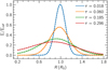 |
Fig. 1 Evolution of the one-dimensional viscously spreading ring. The colors indicate different time stamps, solid lines represent simulation results, and dots follow the analytical solution at the corresponding time according to Eq. (2). |
2.2 Hydrodynamics
We consider the vertically integrated hydrodynamics equations for a gas with surface density Σ, velocity vector u, and nearly zero pressure P at distance R,
 (5)
(5)
The gas orbits around a star with mass M⋆ such that the gravitational potential is given by Φ⋆ = –GM⋆/R, with G being the gravitational constant. The viscous stress tensor is represented with  . We use a locally isothermal equation of state, such that the gas has a (very small) sound speed
  , where h is the aspect ratio.
2.3 Numerical setup
For our standard setup, we used PLUTO version 4.3 (Mignone et al. 2007), a finite-volume code with a second-order accurate scheme (HLLC, Toro et al. 1994) and the van Leer flux limiter (van Leer 1977). We followed the setup laid out in SK03 to reproduce the original results. In this section, we provide a detailed description of our model and its differences with the setup in SK03.
To study the viscous ring and the related instability, we used a polar grid with computational domain R ∈ [0.2,2] R0 and ϕ ∈ [0,2π). We used both logarithmic (ΔR ∝ R) and arithmetic (ΔR = const.) scaling in the radial direction for comparison reasons, but focus on logarithmic setups first. We also enabled the FARGO transport scheme (Masset 2000) implemented in PLUTO by Mignone et al. (2012), while the parabolic viscosity term is handled using the explicit time-stepping method in PLUTO. We used a Courant number of 0.4 in all simulations, unless specified otherwise. The system was then evolved for various grid resolutions, the results of which are discussed in Sect. 3.2. The Cartesian setup used to measure the numerical viscosity is described in Sect. 4.2.
To evolve the viscous ring problem, we initialized the surface density using Eq. (2) at τ0 = 0.018 and added a small, constant surface density floor Σfloor = 10−7 Σref, where Σref = Σring(τ0,1). We chose a set of code units where  . This leaves the kinematic viscosity as the only relevant physical constant in this setup, which we chose to be
  . For this viscosity, we get a viscous ring spreading time (i.e., τ = 1) of 1326 orbital periods (P0) at R = R0. To facilitate development of the spiral instability, the initial surface density distribution was seeded with a small amount of noise and evolved up to t = 400 P0,or τ = 0.3.
We chose a strict outflow boundary condition in both radial directions such that ∂RΣ = 0, uR,in = −|uR(Rin)|, uR,out = |uR(Rout)|. The azimuthal velocity is fixed to the Keplerian speed corrected for pressure support  at the boundaries. We explored various values of the aspect ratio, shown in Appendix A, and chose h = 0.005 for our simulations, as we find it to be low enough for the gas to act like a pressureless fluid and high enough to ensure numerical stability in our simulations. The RH2D setup in SK03 used a viscosity value of
  and an initial viscous time τ0 = 0.016, but this has no effect on the subsequent evolution.
To corroborate our results, we used the FARGO code (legacy version; Masset 2000). Similar to the RH2D code used in SK03, FARGO uses a finite difference scheme as described in Stone & Norman (1992) with the second-order upwind algorithm by van Leer (1977). Both codes therefore show a similar behavior and we used FARGO to compare our results to those of SK03.
3 Analysis of the viscous ring problem
In this section, we explore the spiral instability using logarithmically spaced polar grids. In such grids, the radial cell size ΔR increases with distance such that the ratio ΔR/H remains comparable throughout the domain (in the case of h = const., this ratio is constant as H = hR). This makes logarithmically spaced grids highly suitable for general-purpose disk models, where gas dynamics should be resolved over a scale height H using a reasonable number of cells. We briefly describe the general behavior of the viscous spreading ring and show that our fiducial model is numerically converged.
3.1 Time evolution of the viscous ring
We begin our analysis with a 1D model of the viscously spreading ring, using 465 cells logarithmic scaled in the radial direction. This resolution is chosen such that the gas is resolved with at least one cell per scale height H = hR. Even though the problem is formally defined for a pressureless fluid (h = 0), Figs. 1 and 2 show that our model adequately reproduces the analytical equations of Eqs. (2) and (3), respectively.
To assess the robustness of the numerical methods used, we quantified numerical errors in our results by measuring the average density-weighted relative deviation from the analytical solution of both the surface density Σ and radial velocity uR on the grid, at various times. We find a maximum deviation of 0.74% for Σ and 3.31% for uR. While these values are largely influenced by regions close to the boundaries, where deviations are the largest, for most of the domain (0.4–1.8 R0) we find maximum deviations of 0.15 and 0.75% for Σ and uR respectively. In addition, we find that further reducing the aspect ratio h does not substantially affect the measured errors.
We then expanded to a 2D {R, ϕ} domain, with a fiducial resolution of NR × Nϕ = 465 × 256. Here, we expect the same radial spreading of the ring but also development of the viscosity-driven spiral instability discussed in SK03. Figure 3 shows a time evolution of the ring spreading and of the instability, which manifests in the form of an outward-propagating spiral arm. Weak radial wave-like perturbations are launched immediately after the start of the simulation (see panel a).
The perturbations are not affected by changes to pressure or initial conditions, but they do become weaker and move to smaller wavelengths with lower viscosity. This viscosity dependency is in agreement with the viscous overstability (e.g., Latter & Ogilvie 2006) but a more thorough study of the perturbations is not within the scope of this work.
These initial waves leave the domain through the outer boundary, while the spiral instability begins to develop near the inner boundary, with the spiral becoming apparent at τ ≈ 0.03 (panel b). The spiral continues to grow in amplitude and propagate outwards until it eventually spans the entire radial extent of the disk (panels c,d).
In contrast to the results in SK03, we do not see a flip of the direction of the spiral from leading to trailing around the peak of the ring. Instead, we find that this flip is merely a numerical artifact and does not appear in simulations with a sufficiently high radial resolution. We discuss this further in Appendix B.
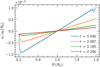 |
Fig. 2 Similar to Fig. 1 showing the evolution of radial velocity of the ring compared to the analytical solution Eq. (3). |
3.2 Resolution study
To ensure a properly resolved and developed viscous instability, we performed a resolution study by analyzing its growth phase. For this, we measured the largest density deviation from the azimuthally averaged profile at different radii and tracked this quantity over time. In that sense, this quantity acts as a proxy for the time evolution of the amplitude of the strongest spiral at a given radius, which hints at the growth rate of the spiral instability. Figure 4 shows this evolution for various resolutions. Alternatively, we also evaluated the amplitude of the azimuthal Fourier modes of density rings at specific radii over time. The results obtained using this method are similar to those obtained from measuring the density deviations and are therefore not shown here.
After comparing our results against a model with square cells (NR × Nϕ = 465 × 1300), we find that increasing the azimuthal resolution beyond 256 cells has no effect on the growth rate of the instability (see Fig. 4b) and therefore fixed the number of azimuthal cells to 256 in our resolution study. In the radial direction we find a resolution of 465 cells to be sufficient.
We confirmed our results using the FARGO code in Appendix B and achieved numerical convergence with both codes at a resolution of 465 × 256 cells. We conclude that this resolution is sufficient to fully resolve the viscously spreading ring and the development and saturation of spiral arms due to the spiral instability.
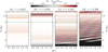 |
Fig. 3 Snapshots of the normalized deviation from the analytical surface density distribution for our fiducial model at different times. The dashed green line marks the position of maximal surface density, which indicates the peak of the spreading ring. Initial waves (a) are seen as outward-moving rings while the spiral instability develops as a spiral arm at the inner boundary (b) and spreads through the whole domain (c,d). |
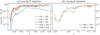 |
Fig. 4 (a) Time evolution of the normalized maximal deviation from the azimuthally averaged surface density distribution for various numerical configurations. Inadequate resolution in the R-direction can damp the viscous instability, with convergence being achieved for our fiducial model with NR = 465. (b) Comparison of the same quantity for different azimuthal resolutions and NR = 465. The higher resolution of Nϕ = 1300 azimuthal cells results in square grid cells but does not influence the growth of the instability. |
4 The viscous ring problem in Cartesian coordinates
Having profiled the viscous ring problem in a polar grid, we now switch to Cartesian coordinates with our ultimate goal being the measurement of the numerical viscosity of PLUTO for such a grid. For this set of models, our computational domain extends between x, y ∈ [−2, 2] R0, with a fiducial resolution of Nx × Ny = 1024 × 1024 cells, which corresponds to approximately one cell per scale height at  . We note that, Δx = Δy = const. in these models, and therefore our effective resolution is significantly lower at smaller radii.
For a fair comparison with our models on a polar grid, we retained the second-order accurate HLLC scheme with a linear spatial reconstruction and van Leer flux limiter for all simulations unless otherwise stated. In addition, we emulated the inner radial boundary of a polar grid using a damping region, where we damped 2 to Σring through Eq. (2) and uR to zero for R < 0.2 R0. Finally, we set an outflow boundary condition at all domain boundaries. To measure numerical viscosity in PLUTO, we used a similar setup but damped Σ to Σfloor following (de Val-Borro et al. 2006), and provide a comparison using Athena++ version 21.0 (Stone et al. 2008).
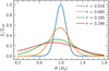 |
Fig. 5 Snapshots of slices through the y = 0 plane showing the evolution of surface density for our fiducial viscous Cartesian simulation. The colors indicate different time stamps, solid lines represent simulation results, and dots follow the analytical solution at the corresponding time according to Eq. (2). Unlike the 2D polar case, no spirals develop. |
4.1 Viscous evolution
We first analyze the evolution of the ring with standard viscosity similar to in Sect. 3. The radial ring spreading and the radial velocity evolution can be seen in Figs. 5 and 6, respectively; they match the analytical solution well except for noticeable deviations in uR close to the damping region and boundaries. We again quantified the error by measuring the density-weighted relative deviations in the domain excluding the damping region and find a maximum deviation of 0.71% for Σ and of 15.74% for uR,ring. We note that, unlike the polar case, we find no development of spirals in any Cartesian model. We suspect that the spiral instability is suppressed as a result of the highly diffusive grid, which is further discussed in Sect. 5. We see similar results at lower and higher resolutions of 5122 and 20482 cells.
4.2 Inviscid models: Estimates of numerical viscosity
The discretization in space and time inherent in the numerical schemes employed by our codes results in numerical errors when solving the hydrodynamics equations. In our analysis in Appendix C, we show that this error has the form of a numerical viscosity and can lead to ring spreading, even in the absence of any physical viscosity. In this section, we repeat the models shown in Sect. 4.1 with an inviscid prescription (v = 0), and analyze the subsequent ring spreading in an attempt to quantify the numerical viscosity of the methods in PLUTO.
Blue lines in Fig. 7 show the time evolution for our fiducial inviscid model at a resolution of 1024 × 1024. We find that the ring spreading is indeed quite similar to viscous models, with the exception that the peak of the ring is flatter compared to the analytical solution. We then extracted a global estimate of the numerical viscosity vnum by fitting the analytical solution Eq. (2) to our data. The fitting method is described in Appendix D.
We repeated the simulation with a prescribed kinematic viscosity equal to the measured numerical viscosity (v = vnum) and once again with v = 2 vnum, the time evolution of which is shown as orange and green lines, respectively, in Fig. 7. We find that the v = vnum model evolves twice as fast as our inviscid model, and the v = 2 vnum model evolves three times as fast. This suggests that all models evolve as if the total viscosity were vtot = v + vnum. We motivate our approach and rationalize this result in Appendix C.
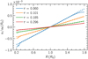 |
Fig. 6 Similar to Fig. 5, showing the evolution of radial velocity of the ring compared to the analytical solution Eq. (3). |
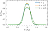 |
Fig. 7 Slices of surface density profiles for our fiducial inviscid Cartesian model (v = 0, blue lines) at a given time t0 against the corresponding viscous models with v = vnum at t0/2 (orange) and v = 2 vnum at t0/3 (green). Solid and dashed lines correspond to t0 = 224 and 748 orbits at R0, respectively. The model with v = vnum evolves twice as fast as the inviscid simulation and the v = 2 vnum model evolves three times as fast, indicating a viscous contribution by the non-negligible numerical viscosity. |
Numerical viscosity vnum with one standard deviation errors in code units for different grid types and resolutions.
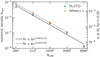 |
Fig. 8 Numerical viscosity |

4.2.1 Resolution scaling of the numerical viscosity
In our analysis of the numerical viscosity for a first-order solver in Appendix C, we show that the numerical viscosity scales as vnum ∝ Δx for a first-order method. As we used a second-order solver for our tests, we expect the numerical viscosity to scale as vnum ∝ Δx2 in our models. To test this, we conducted simulations for grid resolutions of 2562, 5122, 10242, 20482, and 40962 cells. The resulting values of vnum as a function of cell count are listed in Table 1 and shown in Fig. 8. We then fit a power law to the relation vnum(Δx) and find that the numerical viscosity scales as vnum ∝ Δx2.09. We also find that reducing the maximum Courant number Cmax ≈ Δt/min (Δx/u) from our nominal value of 0.4 had no effect on the numerical viscosity, indicating that the dependence of vnum on Δx, Δt, and the Courant number is more complicated than it would be for a first-order scheme. While we find our vnum ∝ Δx2 estimate to roughly describe the convergence, we also find that the convergence rate is not constant and increases with resolution. We obtain similar results using the code Athena++ (see Appendix E).
For a realistic protoplanetary disk with h ~ 0.05, the numerical viscosity  extracted from our fiducial Cartesian model translates to an α viscosity parameter (Shakura & Sunyaev 1973) of
  . More generally, we can write
 (6)
(6)
5 Discussion
In this section, we compare our results on the spiral instability to those found in SK03, and comment on the nature of numerical viscosity.
5.1 Comparison to previous results
Analyzing the spreading ring on a polar grid in Sect. 3, we confirm the main findings from SK03 that the viscous pressureless spreading ring is subject to a viscous instability that manifests as a leading spiral arm. On the other hand, we find the flip from a leading to a trailing spiral described by these latter authors to be purely of numerical origin. As shown in Appendix B, we attribute the spiral flip to an under-resolved inner disk; the quantity ΔR/R increases for small radii in an arithmetic grid like that of SK03, while a constant smoothing length in their SPH simulations results in effectively the same issue. In our adequately resolved models (NR ≥ 465), we find many azimuthal spiral modes growing at the beginning of our simulation with their amplitude decaying exponentially with mode number. However, in our arithmetic, low-resolution analog of SK03, the growth of azimuthal Fourier mode amplitudes is delayed and weaker, and their amplitude decays faster with increasing mode number (Fig. B.2). We provide more details in Appendix B, but conclude here that any effects found by SK03 in addition to the leading spiral are due to the lower numerical resolution used by these authors.
5.2 Differences between physical and numerical viscosity
In Sect. 3.1, we show the development of the spiral instability for our fiducial polar model (Fig. 3) and its growth (Fig. 4). Unlike the polar grid, our Cartesian models do not develop this instability, even at comparatively higher resolutions. This can be attributed to the lack of angular momentum conservation, which results in a dramatically high numerical diffusivity. We confirm this by analyzing the growth rates of the instability as in the polar case in Fig. 9, and show that azimuthal wavenumbers in Cartesian runs saturate at levels that are six orders of magnitude weaker compared to polar runs.
Furthermore, we interpolated our fiducial polar run with a fully developed spiral onto a Cartesian grid and note that the spiral features of the viscous instability completely vanish within a span of 2–4 orbits after continuation. This suggests that even though numerical diffusion causes an effect akin to physical viscosity, the properties of numerical and physical viscosity are not the same. Both physical and numerical viscosity lead to a viscous spreading of the initial ring distribution, whereas a physical viscosity is necessary for the development of the spiral instability. The same effect cannot be replicated by numerical diffusion alone.
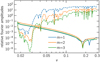 |
Fig. 9 Fourier amplitude normalized to azimuthally averaged density at R = 0.5 R0 for m = 1,2,3 for the fiducial polar simulation (dashed lines) and interpolated fiducial Cartesian simulation (solid lines). The spiral instability does not develop, with amplitudes of up to six orders of magnitude weaker compared to the polar case. |
5.3 Effect of characteristic limiting on numerical viscosity
A commonly used method to reduce diffusive numerical effects is characteristic limiting (CL; implemented by Mignone et al. 2012), whereby spatial reconstruction is performed on characteristic variables instead of the primitive variables in the system. We assessed the effect of this method by comparing to our inviscid 512 × 512 Cartesian simulation with otherwise identical parameters. The low resolution was chosen to highlight the substantial difference while using CL. As shown in Fig. 10, the simulation with CL is less diffusive, which is evidenced by the lack of a flattened peak and a more weakly diffused ring overall. On average, the model with CL has roughly half the numerical viscosity of the standard inviscid 512 × 512 model.
6 Conclusions
We revisited the viscous ring problem in SK03 using the finite-volume codes PLUTO and Athena++ as well as the finite-difference code FARGO in an attempt to measure the numerical viscosity of hydrodynamical codes. We first reproduced the viscous ring spreading in one dimension and the spiral instability in two dimensions on a polar grid. We analyzed the growth of the instability and show that SK03 has insufficient spatial resolution to properly resolve the instability growth.
We then evolved the viscous ring spreading in two dimensions on a Cartesian grid, applying the same viscosity v as used in the polar grid run. The evolution matches the analytical solution to good accuracy but fails to develop the spiral instability even at higher resolutions. We attributed the absence of spiral development to the lack of angular momentum conservation and subsequently high numerical diffusion inherent to Cartesian grids. Our findings suggest that a high physical viscosity is not the only ingredient to developing the spiral instability, and that a numerical setup is needed with very good angular momentum conservation and low numerical diffusivity.
The viscous spreading ring was then used to measure the numerical viscosity in Cartesian grids. This was done by evolving the viscous ring for an inviscid setup and fitting the simulated ring evolution with the analytical solution in Eq. (2) as a function of time. As the ring evolution depends only on the viscosity v, this method allows us to extract the viscosity over which the system evolves, which for an inviscid system is the numerical viscosity. We then show a scaling relation between numerical viscosity and resolution that, for second-order methods, corresponds to  . Translating our results to a Shakura–Sunyaev α parameter, we find a relation
  for our fiducial model with
  and a realistic aspect ratio h = 0.05.
We highlight that our models all utilize second-order accurate schemes in both space and time. Even though the effects of numerical viscosity can be mitigated to some degree by using higher order spatial reconstruction and time-marching algorithms, further investigation of this matter is required.
Our results reveal the existence of moderate diffusive effects in Cartesian grids and quantify the resulting numerical viscosity for standard numerical parameters and different grid resolutions. We also lay out a method that can be used to quantify the numerical viscosity to good accuracy. This information can be used to make informed decisions on how to measure and minimize numerical diffusion in hydrodynamics simulations of accretion disks, and is especially useful in the context of low-viscosity or even inviscid configurations of circumbinary or protoplanetary disks on Cartesian grids, as well as for inherently Cartesian codes.
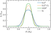 |
Fig. 10 Inviscid Cartesian 5122 simulation utilizing characteristic limiting (dashed line) compared to our standard inviscid models at resolutions of 5122 and 10242 (solid lines) after 150 orbits at R0. Characteristic limiting reduces numerical viscosity by a factor of roughly 2 at 5122 resolution. A dotted black line shows the fit using the analytical ring profile for the 5122 simulation. |
Acknowledgements
We dedicate this paper to the memory of our dear friend and mentor Willy Kley, with whom we developed the idea for this paper. We thank him for his fundamental work, counseling, and kindness. A.Z. and R.P.N. are supported by STFC grant ST/P000592/1, and R.P.N. is supported by the Leverhulme Trust through grant RPG-2018-418. G.A.T. is supported by an STFC PhD studentship. J.J. is co-funded by the European Union (ERC, EPOCH-OF-TAURUS, 101043302). Views and opinions expressed are however those of the author(s) only and do not necessarily reflect those of the European Union or the European Research Council. Neither the European Union nor the granting authority can be held responsible for them. The authors acknowledge support by the High Performance and Cloud Computing Group at the Zentrum für Datenverarbeitung of the University of Tübingen, the state of Baden-Württemberg through bwHPC and the German Research Foundation (DFG) through grant no INST 37/935-1 FUGG. This research utilised Queen Mary’s Apocrita HPC facility, supported by QMUL Research-IT (http://doi.org/10.5281/zenodo.438045). This work was performed using the DiRAC Data Intensive service at Leicester, operated by the University of Leicester IT Services, which forms part of the STFC DiRAC HPC Facility (www.dirac.ac.uk). The equipment was funded by BEIS capital funding via STFC capital grants ST/K000373/1 and ST/R002363/1 and STFC DiRAC Operations grant ST/R001014/1. DiRAC is part of the National e-Infrastructure. The plots in this paper were prepared using the Python library matplotlib (Hunter 2007).
Appendix A Effect of pressure scale height on the viscous ring spreading and spiral instability
The analytical solution for the viscous ring spreading and the stability analysis of the spiral instability studied in SK03 assumes a disk without pressure. For a locally isothermal system, this would imply an aspect ratio of h = 0 but the PLUTO solver becomes numerically unstable under this condition. To ensure that the pressure in our simulations is small enough to properly simulate the spiral instability, we compared the maximal spiral amplitude time averaged over τ = 0.2–0.3 for different values of aspect ratio h in Fig. A.1.
For aspect ratios h > 0.006, the spiral instability is strongly damped and the ring structure deviates substantially from the analytical solution. For aspect ratios h < 0.006, the instability becomes stronger, and is fully saturated at our fiducial aspect ratio of h = 0.005. We also tested and confirmed (not shown) that the numerical viscosity measured in our Cartesian runs is fully converged for h = 0.005. Nevertheless, our fiducial aspect ratio is small enough for the gas to be considered pressureless, and we found that the noise we observed in the amplitude of the instability (see e.g., Fig. 4) fades away for even lower aspect ratios and the time evolution becomes smoother, as is the case in our FARGO simulations (see Fig. B.1).
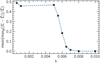 |
Fig. A.1 Time average of the maximal spiral amplitude at R = 0.5 R0 between τ = 0.2–0.3 for different values of aspect ratio h. The spiral instability is strongly damped for h > 0.006 while spiral amplitudes converge for h < 0.005. |
Appendix B Comparison of codes and the spiral flip in SK03
To test the robustness of our results on the spiral instability we performed a similar suite of simulations using the FARGO code. Figure B.1 shows the growth of the spiral instability for different resolutions. We see that a resolution of 465 × 256 is sufficiently converged, with full convergence at 1024 × 256 and above. Even though PLUTO achieved convergence at a lower resolution of 465 × 256, FARGO shows slight improvements in the growth onset and amplitudes for higher resolutions. Regardless, we can conclude that the results are consistent between both codes. We note that just like PLUTO, the spiral flip vanishes before it reaches the ring in FARGO simulations for resolutions with more that 465 radial cells.
To further understand the spiral flip results shown in SK03 we replicated their setup in FARGO, with a 256 × 256 arithmetically spaced polar grid. Our simulation reproduces their Fig. 6 very well, but is run for longer. The spiral flip pattern emerges after τ = 0.04 and gradually morphs into a single leading spiral for τ > 0.43 (see Fig. B.3). We conducted additional simulations with higher resolutions and also on logarithmic grids. Each time the resolution was increased on an arithmetic grid, the flip occurred further inward and turns into a leading spiral earlier in the simulation. On a logarithmic grid, the inner region is better resolved and the flip always vanishes early in the simulation and never reaches the spreading ring; see Fig. B.3.
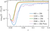 |
Fig. B.1 Time evolution of the normalized maximal deviation from the initial surface density distribution for different FARGO simulations compared to the fiducial PLUTO simulation. |
A comparison of the growth rates between the SK03 setup and a high-resolution FARGO run is shown in Fig. B.2. As the grid is the only difference between the simulations, the flip seems to be a numerical effect that is exacerbated when using an arithmetic grid, which has a lower resolution at the inner boundary. The constant smoothing length used for the SPH code in SK03 has the same resolution effect as an arithmetic grid, which explains why their simulations are in agreement. We conclude that the flipped spiral structure with a trailing spiral observed at the inner domain in SK03 is merely a numerical effect.
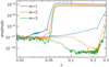 |
Fig. B.2 Time evolution of the first three Fourier azimuthal modes at R = R0. Solid lines represent a high-resolution (2048 × 256) simulation using a logarithmic grid, and the dashed lines represent results from an identical setup as in SK03, with a 256 × 256 arithmetic grid. |
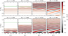 |
Fig. B.3 Surface density deviation heat maps similar to Fig. 3, but for FARGO simulations at a resolution of 256 × 256 on an arithmetic grid (top) and at 456 × 256 on a logarithmic grid (bottom). Top: Setup that reproduces the results of SK03 (see Fig. 6 therein). The flip from a leading to trailing spiral is visible in the middle two panels, before it disappears into a single leading spiral. Bottom: Setup that is equivalent to our fiducial PLUTO model, and behaves very similar to our results in Fig. 3. Here, spirals develop earlier and the initial flip is short-lived and closer to the inner boundary. |
Appendix C Numerical diffusion as a consequence of advection
We consider the 1D advection equation of a quantity q for a fluid moving at constant velocity u > 0
 (C.1)
(C.1)
We can discretize this equation to a first-order upwind scheme (e.g., Courant et al. 1952) where q′ = q(t + Δt) on a grid where i is the cell index such that qi–1 = q(xi – Δx)
 (C.2)
(C.2)
By Taylor-expanding  and qi–1 to second order in time and space respectively, and substituting a wave-like solution qtt = uqxx, we arrive at a modified upwind equation:
 (C.3)
(C.3)
which corresponds to an advection–diffusion equation with diffusion coefficient D. This term, while not physically motivated, allows the upwind scheme to remain stable for Courant numbers 0 < C < 1.
This approach does not exactly relate to our results, because the gas velocity is not constant and we further use second-order schemes with PLUTO. Nevertheless, we can expect that our numerical scheme will give rise to a similarly-motivated numerical diffusion term such that Eq. (5) effectively becomes
 (C.4)
(C.4)
with  and
and  . Given that our inviscid Cartesian models behave similarly to viscous models with viscosity vnum as far as ring spreading is concerned, it is therefore unsurprising that a ring in a viscous model with v ~ vnum should spread as if the total viscosity were vtot ≈ v + vnum.
We also note that, for a given Courant number C, the diffusion coefficient in Eq. (C.3) is proportional to Δx for the first-order method we considered, and expect a Δx2 scaling for a second-order method in 1D. Given that the viscous ring problem evolves on both the x and y directions in 2D, doubling the resolution would require increasing the number of cells in both directions by a factor of 2 (thus increasing grid cell count by a factor of 4). In doing so, we would expect a scaling vnum ∝ Δx2, which is verified in Fig. 8.
Finally, we found that doubling the resolution in only one direction (such as Nx × Ny = 512 × 1024) results in a numerical viscosity estimate that is much closer to the value expected for the low-resolution direction (in this case, Nx) than to an estimate dictated by Δx × Δy. This rules out that the numerical diffusion we observe depends linearly on Δx and Δy and suggests that it more accurately depends on max(Δx, Δy)2, highlighting the second-order accuracy of our solver.
Appendix D Measuring numerical viscosity
To measure the numerical viscosity in our inviscid simulations we utilize the relation between the viscous timescale τ for the ring spreading and the orbital time t at R0 given by  . We note that for a given viscosity v, this equation represents the slope–intercept form of an equation for a line with slope
  and intercept zero.
To do so, first we fit the analytical solution to a slice of the two-dimensional data at time t to compute τ. Repeating this procedure for all snapshots generates a curve for τ(t) shown in Fig. D.1. We then fit a straight line to the τ(t) curve for approximately the last 180 orbits. The slope of this straight line fit gives the numerical viscosity using the above relation for the slope m.
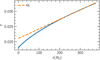 |
Fig. D.1 The τ(t) curve for our inviscid 1024 model. The dashed line shows the fit over the last 180 time units. The slope of this line is used to extract the numerical viscosity. |
Appendix E Inviscid Cartesian simulations with Athena++
For the suite of Cartesian models using Athena++, we implement an equivalent setup to the PLUTO runs, as described in Sect. 2. A locally isothermal disk is achieved by using an adiabatic equation of state combined with a thermal relaxation timescale  . The viscous ring sits on top of a constant density background with Σbgr = 10−7 Σref, however the density floor of the domain was set to Σfloor = 10−15 Σref as interactions with the density floor created numerical instabilities.
Our results are listed in Table 1 and shown in Fig. 8. Both codes agree very well for Ncells ≥ 10242, which corresponds to our fiducial resolution. The expected behavior of vnum ∝ Δx2 is also found with Athena++.
References
- Andrews, S. M., Huang, J., Pérez, L. M., et al. 2018, ApJ, 869, L41 [NASA ADS] [CrossRef] [Google Scholar]
- Bai, X.-N., & Stone, J. M. 2013, ApJ, 769, 76 [Google Scholar]
- Balbus, S. A., & Papaloizou, J. C. B. 1999, ApJ, 521, 650 [Google Scholar]
- Courant, R., Isaacson, E., & Rees, M. 1952, Commun. Pure Appl. Math., 5, 243 [CrossRef] [Google Scholar]
- Crida, A., Baruteau, C., Kley, W., & Masset, F. 2009, A & A, 502, 679 [NASA ADS] [CrossRef] [EDP Sciences] [Google Scholar]
- de Val-Borro, M., Edgar, R. G., Artymowicz, P., et al. 2006, MNRAS, 370, 529 [Google Scholar]
- Dullemond, C. P., Birnstiel, T., Huang, J., et al. 2018, ApJ, 869, L46 [NASA ADS] [CrossRef] [Google Scholar]
- Dullemond, C. P., Ziampras, A., Ostertag, D., & Dominik, C. 2022, A & A, 668, A105 [NASA ADS] [CrossRef] [EDP Sciences] [Google Scholar]
- Flebbe, O., Muenzel, S., Herold, H., Riffert, H., & Ruder, H. 1994, ApJ, 431, 754 [Google Scholar]
- Fromang, S., Hennebelle, P., & Teyssier, R. 2006, A & A, 457, 371 [Google Scholar]
- Haisch, K. E. Jr., Lada, E. A., & Lada, C. J. 2001, ApJ, 553, L153 [NASA ADS] [CrossRef] [Google Scholar]
- Hunter, J. D. 2007, Comput. Sci. Eng., 9, 90 [NASA ADS] [CrossRef] [Google Scholar]
- Kley, W. 1989, A & A, 208, 98 [NASA ADS] [Google Scholar]
- Kley, W. 1999, MNRAS, 303, 696 [NASA ADS] [CrossRef] [Google Scholar]
- Latter, H. N., & Ogilvie, G. I. 2006, MNRAS, 372, 1829 [NASA ADS] [CrossRef] [Google Scholar]
- Lega, E., Morbidelli, A., Nelson, R. P., et al. 2022, A & A, 658, A32 [NASA ADS] [CrossRef] [EDP Sciences] [Google Scholar]
- Lüst, R. 1952, Zeitschrift Naturforschung Teil A, 7, 87 [CrossRef] [Google Scholar]
- Lynden-Bell, D., & Pringle, J. E. 1974, MNRAS, 168, 603 [Google Scholar]
- Lyra, W., & Umurhan, O. M. 2019, PASP, 131, 072001 [Google Scholar]
- Masset, F. 2000, A & AS, 141, 165 [NASA ADS] [Google Scholar]
- Mignone, A., Bodo, G., Massaglia, S., et al. 2007, ApJS, 170, 228 [Google Scholar]
- Mignone, A., Zanni, C., Tzeferacos, P., et al. 2012, ApJS, 198, 7 [Google Scholar]
- Pringle, J. E. 1981, ARA & A, 19, 137 [NASA ADS] [CrossRef] [Google Scholar]
- Shakura, N. I., & Sunyaev, R. A. 1973, A & A, 24, 337 [NASA ADS] [Google Scholar]
- Speith, R., & Kley, W. 2003, A & A, 399, 395 [CrossRef] [EDP Sciences] [Google Scholar]
- Stone, J. M., & Norman, M. L. 1992, ApJS, 80, 753 [Google Scholar]
- Stone, J. M., Gardiner, T. A., Teuben, P., Hawley, J. F., & Simon, J. B. 2008, ApJS, 178, 137 [NASA ADS] [CrossRef] [Google Scholar]
- Tiede, C., Zrake, J., MacFadyen, A., & Haiman, Z. 2022, ApJ, 932, 24 [NASA ADS] [CrossRef] [Google Scholar]
- Toro, E. F., Spruce, M., & Speares, W. 1994, Shock Waves, 4, 25 [Google Scholar]
- van Leer, B. 1977, J. Comput. Phys., 23, 276 [Google Scholar]
- Zhang, S., Zhu, Z., Huang, J., et al. 2018, ApJ, 869, L47 [Google Scholar]
- Zier, O., & Springel, V. 2022, MNRAS, 515, 525 [NASA ADS] [CrossRef] [Google Scholar]
All Tables
Numerical viscosity vnum with one standard deviation errors in code units for different grid types and resolutions.
All Figures
|
Fig. 1 Evolution of the one-dimensional viscously spreading ring. The colors indicate different time stamps, solid lines represent simulation results, and dots follow the analytical solution at the corresponding time according to Eq. (2). |
| In the text | |
|
Fig. 2 Similar to Fig. 1 showing the evolution of radial velocity of the ring compared to the analytical solution Eq. (3). |
| In the text | |
|
Fig. 3 Snapshots of the normalized deviation from the analytical surface density distribution for our fiducial model at different times. The dashed green line marks the position of maximal surface density, which indicates the peak of the spreading ring. Initial waves (a) are seen as outward-moving rings while the spiral instability develops as a spiral arm at the inner boundary (b) and spreads through the whole domain (c,d). |
| In the text | |
|
Fig. 4 (a) Time evolution of the normalized maximal deviation from the azimuthally averaged surface density distribution for various numerical configurations. Inadequate resolution in the R-direction can damp the viscous instability, with convergence being achieved for our fiducial model with NR = 465. (b) Comparison of the same quantity for different azimuthal resolutions and NR = 465. The higher resolution of Nϕ = 1300 azimuthal cells results in square grid cells but does not influence the growth of the instability. |
| In the text | |
|
Fig. 5 Snapshots of slices through the y = 0 plane showing the evolution of surface density for our fiducial viscous Cartesian simulation. The colors indicate different time stamps, solid lines represent simulation results, and dots follow the analytical solution at the corresponding time according to Eq. (2). Unlike the 2D polar case, no spirals develop. |
| In the text | |
|
Fig. 6 Similar to Fig. 5, showing the evolution of radial velocity of the ring compared to the analytical solution Eq. (3). |
| In the text | |
|
Fig. 7 Slices of surface density profiles for our fiducial inviscid Cartesian model (v = 0, blue lines) at a given time t0 against the corresponding viscous models with v = vnum at t0/2 (orange) and v = 2 vnum at t0/3 (green). Solid and dashed lines correspond to t0 = 224 and 748 orbits at R0, respectively. The model with v = vnum evolves twice as fast as the inviscid simulation and the v = 2 vnum model evolves three times as fast, indicating a viscous contribution by the non-negligible numerical viscosity. |
| In the text | |
|
Fig. 8 Numerical viscosity |
| In the text | |
|
Fig. 9 Fourier amplitude normalized to azimuthally averaged density at R = 0.5 R0 for m = 1,2,3 for the fiducial polar simulation (dashed lines) and interpolated fiducial Cartesian simulation (solid lines). The spiral instability does not develop, with amplitudes of up to six orders of magnitude weaker compared to the polar case. |
| In the text | |
|
Fig. 10 Inviscid Cartesian 5122 simulation utilizing characteristic limiting (dashed line) compared to our standard inviscid models at resolutions of 5122 and 10242 (solid lines) after 150 orbits at R0. Characteristic limiting reduces numerical viscosity by a factor of roughly 2 at 5122 resolution. A dotted black line shows the fit using the analytical ring profile for the 5122 simulation. |
| In the text | |
|
Fig. A.1 Time average of the maximal spiral amplitude at R = 0.5 R0 between τ = 0.2–0.3 for different values of aspect ratio h. The spiral instability is strongly damped for h > 0.006 while spiral amplitudes converge for h < 0.005. |
| In the text | |
|
Fig. B.1 Time evolution of the normalized maximal deviation from the initial surface density distribution for different FARGO simulations compared to the fiducial PLUTO simulation. |
| In the text | |
|
Fig. B.2 Time evolution of the first three Fourier azimuthal modes at R = R0. Solid lines represent a high-resolution (2048 × 256) simulation using a logarithmic grid, and the dashed lines represent results from an identical setup as in SK03, with a 256 × 256 arithmetic grid. |
| In the text | |
|
Fig. B.3 Surface density deviation heat maps similar to Fig. 3, but for FARGO simulations at a resolution of 256 × 256 on an arithmetic grid (top) and at 456 × 256 on a logarithmic grid (bottom). Top: Setup that reproduces the results of SK03 (see Fig. 6 therein). The flip from a leading to trailing spiral is visible in the middle two panels, before it disappears into a single leading spiral. Bottom: Setup that is equivalent to our fiducial PLUTO model, and behaves very similar to our results in Fig. 3. Here, spirals develop earlier and the initial flip is short-lived and closer to the inner boundary. |
| In the text | |
|
Fig. D.1 The τ(t) curve for our inviscid 1024 model. The dashed line shows the fit over the last 180 time units. The slope of this line is used to extract the numerical viscosity. |
| In the text | |
Current usage metrics show cumulative count of Article Views (full-text article views including HTML views, PDF and ePub downloads, according to the available data) and Abstracts Views on Vision4Press platform.
Data correspond to usage on the plateform after 2015. The current usage metrics is available 48-96 hours after online publication and is updated daily on week days.
Initial download of the metrics may take a while.