| Issue |
A&A
Volume 677, September 2023
|
|
|---|---|---|
| Article Number | A167 | |
| Number of page(s) | 19 | |
| Section | Astronomical instrumentation | |
| DOI | https://doi.org/10.1051/0004-6361/202347073 | |
| Published online | 22 September 2023 | |
Deep-learning-based radiointerferometric imaging with GAN-aided training
1
Astroparticle Physics, TU Dortmund University,
Otto-Hahn-Straße 4a,
44227
Dortmund, Germany
e-mail: This email address is being protected from spambots. You need JavaScript enabled to view it.
; This email address is being protected from spambots. You need JavaScript enabled to view it.
2
Hamburger Sternwarte, University of Hamburg,
Gojenbergsweg 112,
21029
Hamburg, Germany
3
Center for Data and Computing in Natural Sciences (CDCS),
Notkestrasse 9,
22607
Hamburg, Germany
4
Section for Biomedical Imaging, University Medical Center Hamburg-Eppendorf,
20246
Hamburg, Germany
5
Institute for Biomedical Imaging, Hamburg University of Technology,
21073
Hamburg, Germany
6
Deutsches Elektronen-Synchrotron DESY,
Notkestraße 85,
22607
Hamburg, Germany
Received:
2
June
2023
Accepted:
24
July
2023
Abstract
Context. The incomplete coverage of the spatial Fourier space, which leads to imaging artifacts, has been troubling radio interferometry for a long time. The currently best technique is to create an image for which the visibility data are Fourier-transformed and to clean the systematic effects originating from incomplete data in Fourier space. We have shown previously how super-resolution methods based on convolutional neural networks can reconstruct sparse visibility data.
Aims. The training data in our previous work were not very realistic. The aim of this work is to build a whole simulation chain for realistic radio sources that then leads to an improved neural net for the reconstruction of missing visibilities. This method offers considerable improvements in terms of speed, automatization, and reproducibility over the standard techniques.
Methods. We generated large amounts of training data by creating images of radio galaxies with a generative adversarial network that was trained on radio survey data. Then, we applied the radio interferometer measurement equation in order to simulate the measurement process of a radio interferometer.
Results. We show that our neural network can faithfully reconstruct images of realistic radio galaxies. The reconstructed images agree well with the original images in terms of the source area, integrated flux density, peak flux density, and the multiscale structural similarity index. Finally, we show that the neural net can be adapted for estimating the uncertainties in the imaging process.
Key words: galaxies: active / radio continuum: galaxies / methods: data analysis / techniques: image processing / techniques: interferometric
© The Authors 2023
 Open Access article, published by EDP Sciences, under the terms of the Creative Commons Attribution License (https://creativecommons.org/licenses/by/4.0), which permits unrestricted use, distribution, and reproduction in any medium, provided the original work is properly cited.
This article is published in open access under the Subscribe to Open model. This email address is being protected from spambots. You need JavaScript enabled to view it. to support open access publication.
1 Introduction
In modern astronomy, radio interferometry plays a unique role because it acquires the highest resolutions of astrophysical sources. This resolution comes at the cost of low data coverage, which generates artifacts in the resulting source images. Therefore, the cleaning of these artifacts is an unavoidable data-processing task for radio interferometric data.
The currently best-working radio interferometers, such as the LOw-Frequency ARray (LOFAR; van Haarlem et al. 2013), record terabytes of data per day. This high data rate is expected to increase substantially for the Square Kilometre Array (SKA; Grainge et al. 2017). In order to analyze the large amounts of data on reasonable timescales, existing analysis strategies must be adapted. Here, machine-learning techniques are a promising way to speed up and simplify existing imaging pipelines. Especially deep learning, which is known for its fast execution times on image data, can accelerate the analysis of large data volumes.
In recent months, an increasing number of deep-learning techniques have been applied to radio interferometer data. Application examples include source detection techniques for three-dimensional Atacama Large Millimeter/submillimeter Array (ALMA) data (Delli Veneri et al. 2022) and the resolution improvements of the Event Horizon Telescope (EHT) image of the black hole in M87 using principal-component interferometric modeling (PRIMO; Medeiros et al. 2023).
We have developed a deep-learning-based imaging approach for radio interferometric data published as the Python package radionets (Schmidt et al. 2023). Our imaging approach uses convolutional neural networks known from super-resolution applications (Ledig et al. 2016) to reconstruct missing visibility data from sparse radio interferometer layouts. Consequently, our deep-learning approach is no classical cleaning, as applied in the CLEAN algorithm (Clark 1980). Instead, we perform the data reconstruction directly in Fourier space. The results presented in this paper build on our previous work (Schmidt et al. 2022). Here, we describe a new method for simulating images with generative adversarial networks (GANs), introduce an enhanced radio interferometer simulation chain based on the radio interferometer measurement equation (RIME), and improve diagnostics.
Figure 1 provides an overview of all parts of our analysis chain. The training of deep-learning models requires large amounts of training data, which we provide by simulating radio galaxies in image space. We use the GAN that was developed and trained by Kummer et al. (2022); Rustige et al. (2023) to create source distributions based on the Faint Images of the Radio Sky at Twenty-Centimeters (FIRST) survey (Becker et al. 1995). In a second step, we employ the RIME framework to simulate radio interferometric observations of these sources. The RIME simulation routine is made available in the python package pyvisgen (Schmidt et al. 2020). During this simulation step, the data are converted from image space into Fourier space because radio interferometers measure complex visibilities. We create training and validation data sets consisting of incomplete uv planes. Then, we train our neural network model to reconstruct the missing visibility data. In the following step, dedicated test data sets are used to evaluate the reconstruction ability of the trained model. By applying the inverse Fourier transformation to the reconstructed visibility data, we recover the source distribution in image space. Thus we can compare the computed reconstruction to the simulated source distribution. Furthermore, we evaluate the source reconstructions with different metrics, such as the area ratio or the intensity ratio of the simulation and reconstruction. A comparison with the established imaging software WSCLEAN (Offringa et al. 2014) is performed to compare application times and reconstruction quality.
In Sect. 2, we introduce the framework created by Kummer et al. (2022); Rustige et al. (2023), which provides the radio galaxy simulations. The additional simulation techniques used to create visibilities are described in Sect. 3. Section 4 lists the changes made to our neural network model in comparison to Schmidt et al. (2022) and the hyperparameters we set for the training process. In Sect. 5, we explain our evaluation techniques. Our upcoming projects and ideas are presented in Sect. 6. In Sect. 7, we summarize our results and conclude.
 |
Fig. 1 Analysis chain used in this work. The analysis chain handles data in image space (green) and Fourier space (orange). It is structured in three parts: simulations, neural network model, and evaluation. |
2 GAN simulations
We used the framework presented in Kummer et al. (2022); Rustige et al. (2023) to improve the quality and authenticity of the simulated radio sources that were used as training data. The simulation technique is based on a generative model. These models are able to learn the underlying statistical distribution of the data and can be used for simulations by sampling from this distribution. In our neural-network-based setup, a GAN (Goodfellow et al. 2014; Salimans et al. 2016) is trained in a supervised way on observations from the FIRST survey (Becker et al. 1995). The data were recorded by the Very Large Array (VLA) in New Mexico with a resolution of 5”. The training data set of this generative model was presented in Griese et al. (2023) and is publicly available (Griese et al. 2022). The two neural networks in the standard GAN setup are called generator and discriminator. The generator generates simulated images from a noise vector, and the discriminator discriminates between real and simulated images. Both are trained simultaneously in a two-player minimax game. Eventually, the generator learns to generate images, which are hardly distinguishable from the training images. The setup we used is shown in Fig. 2.
We employed an advanced version of the standard GAN setup, namely a Wasserstein GAN (wGAN). The Wasserstein distance is used in the main term of the loss function. The discriminator is replaced by a critic that is used to estimate the Wasserstein distance between real and generated images (Arjovsky et al. 2017). Additionally, the two neural networks of our wGAN setup are conditioned on the morphological class label. Hence, the generator can be used to simulate images of specific classes. For the further development of our image reconstruction technique, we employ the generator of the wGAN trained for augmenting classifier training in Rustige et al. (2023). This setup can be used to simulate radio sources of four different morphological classes, namely Fanaroff-Riley Class I (FRI) and Fanaroff-Riley Class II (FRII), which are used for this paper, and “bent” and “compact”. As the model was trained on FIRST images, the generated images have similar properties as the training set of the wGAN. For details of the model training, we refer to Rustige et al. (2023).
We simulated 30 000 FRI sources and 30 000 FRII sources to construct a data set that we split into a 5:1 ratio for the training and validation data. We simulated 10 000 additional sources to create a test data set. They were split into 5000 FRI and 5000 FRII sources. The morphological classes of the Fanaroff-Riley classification scheme are distinguished based on the peak location and properties of the radio emission and are well established in radio astronomy (Fanaroff & Riley 1974). A different generator model was used to simulate each class. Consequently, we ensured that the model was optimally chosen for the given class. The noise in the training data was reduced by setting all pixel values below three times the local root mean square (RMS) noise to the value of this threshold. Subsequently, the pixel values were rescaled to the range between −1 and 1 to represent floating-point grayscale images. The generated images reproduced the preprocessed noise level of the training data inherently. The output size of the images was variable, but in the following, we set it to 128 px × 128 px. However, the generated images required some postprocessing: Gaussian smoothing was applied to the images because strong variations exist between neighboring pixels around the sources, that is, low-intensity pixels lie directly next to high-intensity pixels. The width of the Gaussian had to be chosen such that the peaks of the main sources were not smeared out and substructures in the images were not eradicated. We decided to use a width of σ = 0.75 px, which best fulfills the previously mentioned criteria. A comparison of different σ values for the same example wGAN-generated source is shown in Fig. B.1. After this, the sources were scaled between 1 mJy and 300 mJy. Thus, we ensured that the signal-to-noise ratios (S/Ns) ranged between 1 and 100. The S/Ns were defined with the help of WSCLEAN. We performed a cleaning until we reached the threshold of 5 σ (see the auto-mask option of WSCLEAN). We then compared the maximum of the clean image with the standard deviation of the residual image. Tests with different simulation options revealed that flux densities between 1 mJy and 300 mJy lead to S/Ns between 1 and 100 in the simulated observations for our chosen setup. A detailed analysis for data with different S/Ns and additional information about the S/N calculation can be found in Sect. 5.1.
 |
Fig. 2 Schematics of the wGAN architecture reproduced from Rustige et al. (2023), where y denotes the class label of real x or generated images |

3 RIME simulations
The keys to a deep-learning-based analysis of radio observations are the training data sets for the deep-learning models. An accurate simulation chain is essential for the training data to have the same properties as actual measurements. In addition to the source simulations (see Sect. 2), the simulation of the radio interferometer plays a central role and forms the second large block in our analysis chain that we present in Fig. 1. To describe the signal path from the sources toward measured data, we used the radio interferometer measurement equation (RIME; Smirnov 2011). The RIME uses Jones matrices (Hamaker et al. 1996) to process the source signals. For each corruption effect, a new Jones matrix is defined. The GAN-simulated sources described in Sect. 2 are the input for the RIME calculations. Matrices are marked with bold letters in the following.
Because we focus on imaging tasks, we assumed calibrated data for our simulations. No direction-dependent effects were therefore taken into account. Hence, only the geometric signal delay between the antennas and the characteristic of the individual antenna responses were considered. Thus, the RIME for calculating the complex visibility measured by the antenna pair pq at time t is
 (1)
(1)
Here, B(l, m) describes the brightness distribution of the source given in the direction cosines l, m. At this stage, we did not simulate polarization data. The generated visibilities correspond to full intensity data, known as Jones I. Furthermore, K(l, m) describes the phase-delay kernel, defined as
 (2)
(2)
The phase-delay kernel takes into account the propagation lengths of the signal to the different telescopes inside the interferometer array. While (l, m) are used to describe the source distribution, the antenna positions are given in the direction cosines (u, v). The effects of the phase-delay kernel K(l, m) for different baseline lengths is illustrated in Fig. F.1. The characteristics of the VLA 25 m antennas are encoded in E(l, m), which is defined as
 (3)
(3)
with
 (4)
(4)
Again, (u, v) and (l, m) are the coordinate system in Fourier and image space, respectively. Furthermore, the telescope diameter d and the angular distance between pointing position and source structure θlm were considered. J1 is the Bessel function of the first kind (Smirnov 2011). The telescope response E(l, m) is illustrated in Fig. F.2. corresponds to the conjugate transpose of the matrix Xq. We summed over all image pixels to calculate one complex visibility.
In this analysis, we used the B-configuration layout of the VLA, which was used for the FIRST observations. The antenna positions are listed in Table E.1. The RIME enabled us to simulate exact (u, v) coverages. Figure 3 shows a simulated (u, v) coverage using the above RIME formalism. One of the characteristics of the VLA is directly visible in this image: While the center of the image is well covered, the edges are poorly sampled because the baselines are relatively short compared to those of the VLBA, for instance. This property complicates the reconstruction at the edge of the visibility space.
Because real observation depend on multiple observation parameters such as the correlator integration time or the number of scans per pointing, these parameters can be altered in our simulation framework. Table 1 summarizes the parameters we used for the simulations. When multiple values are specified, these values serve as bounds of random values that are drawn within these bounds. The parameters were altered for each new simulated observation.
An additional corruption effect that occurs during radio interferometer observations results from the system noise. This noise effect changes when different bandwidths or correlator accumulation times are used. The noise originating from a specific measurement process is Gaussian distributed with a standard deviation that is defined by
 (5)
(5)
Here, ηs is the system efficiency factor, Δν corresponds to the observation bandwidth, τacc is the correlator accumulation time, and SSE denotes the system equivalent flux density (Taylor et al. 1999). Values for Δν and τacc were taken from Table 1, while ηs = 0.93 and SSE = 420 Jy were taken from the VLA specifications NRAO (2023). The noise drawn in this way, which is about 10 mJy, was added to the real and the imaginary part of the simulated visibilities. This noise-handling technique enables the simulation of observed radio galaxies with different signal-to-noise ratios depending on the peak flux densities of the simulated radio galaxies.
Finally, the visibilities were saved to FITS files together with the meta data of the simulated observations. We used our implementation of a FITS writer, which follows the specifications in AIPS Memo 1171. Saving the simulations in this way means that they can be read and interpreted by established imaging tools such as CASA (The CASA Team et al. 2022) and WSCLEAN (Offringa et al. 2014).
Both established imaging software and our deep-learning-based approach require input data on a regular grid or two-dimensional image data. Therefore, the simulated visibilities have to be gridded. In the context of the RIME simulations, we implemented our own gridder, which is slightly different from the established approach. As with the gridder implemented in WSCLEAN, the grid can be defined with the help of the selected pixel size and number of pixels. Our implementation then does not perform a convolutional gridding, as WSCLEAN does, but we apply a two-dimensional histogram to grid the visibilities. In this work, we chose a pixel size 1.56″ and an image size of 128 px × 128 px, which corresponds to a field of view of 200″.
We have published our simulation routine as an open-source Python package called pyvisgen (Schmidt et al. 2020). With this RIME simulation framework, we built a flexible basis for future simulations of radio interferometer observations. Different corruption effects can easily be added. Furthermore, our method can readily be adapted for other radio interferometer arrays by updating the interferometer characteristics and the antenna positions.
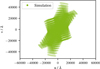 |
Fig. 3 Exemplary (u, v) coverage of a VLA simulation using the developed RIME implementation. |
Observation parameters we applied to simulate the data sets.
4 Deep-learning-based imaging
We imaged the radio interferometer data using deep-learning techniques available inside the Python package radionets (Schmidt et al. 2023). Our approach differs from the conventional CLEAN algorithm (Clark 1980) in that we reconstruct missing information directly in Fourier space. In the reconstruction process, no iterative source model is formed. Consequently, no convolution with the clean beam of the observation is necessary.
The missing data in Fourier space are reconstructed by the trained deep-learning model. The model exploits the data that were recorded during an observation and uses the information they contain to estimate values for missing pixels with the help of convolutional layers (Goodfellow et al. 2016). We described the underlying method in our previous publication (Schmidt et al. 2022). In the following, we discuss the changes we made for the simulated FIRST data.
4.1 Model definition
Our imaging architecture was based on residual blocks (He et al. 2015; Gross & Wilber 2016) integrated into a SRResNet architecture known from super-resolution problems (Ledig et al. 2016). A detailed model description can be found in Schmidt et al. (2022). We kept the original architecture, but increased the number of residual blocks to 16 because as the complexity of the input images increases, as described in the previous sections, the depth and complexity of the network must also increase in order to obtain meaningful reconstructions.
4.2 Model training
Because our deep-learning-based imaging is performed directly in Fourier space, the deep-learning model was trained in Fourier space as well. The simulated visibilities, described in Sect. 3, were used as input. During the training process, the model learned to reconstruct missing information and generated complete real and imaginary maps as output. Figure 4 gives an overview of this training routine.
To train the model, we used a data set consisting of 70 000 real and imaginary images. 50 000 of these images were used to train the neural network. An additional 10 000 validation maps helped us to check for overtraining. In Sect. 5, the remaining 10 000 images are used to evaluate the trained model. In one training epoch, all training and validation maps were passed through the network. The loss function that quantifies the difference between the network prediction and the simulated truth was chosen to be a split L1 loss (6), which is defined as
 (6)
(6)
with
 (7)
(7)
where x is the predicted output from the network, and y is the true distribution.
We used the ADAM optimizer (Kingma & Ba 2014) to update the weights during training, which outperformed the stochastic gradient decent (SGD; Amari 1993) in convergence time at the cost of more readily learned parameters. We trained the neural network model for 400 epochs with a batch size of 100. An adaptive learning rate was applied, starting with a learning rate of 2 × 10⁻⁴, which peaked after 150 epochs at 1 × 10⁻³. The learning rate then steadily decreased to 6 × 10⁻⁴ until the end of the training. The duration of one epoch was 185 s, which resulted in a total training time of ≈20.5 h on the computing specifications summarized in Table D.1. The reconstruction times of the neural network model were some milliseconds. For a 128 px × 128 px image, the pure reconstruction time of the neural network was (6.4 ± 0.1) ms evaluated 100 times on the same image. As our approach has no iterative routines, the reconstruction time was independent of the (u, v) coverage. A reconstruction time comparison with established imaging software is given in Sect. 5.2.
Figure 5 visualizes the curves for the training and validation loss. The training and validation losses steadily decrease in both cases. A gap between training and validation loss starts to form after the first about ten epochs. However, this gap is not a sign of overtraining because the validation loss does not start to increase in later epochs.
We were able to smooth the loss curves by implementing a normalization based on all training images. Here, the mean of all nonzero input values was subtracted from all nonzero pixels. In the next step, the result was divided by the standard deviation of all nonzero values. The complete normalization is defined as
 (8)
(8)
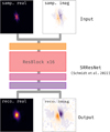 |
Fig. 4 Overview of the training routine. |
4.3 Reconstruction
In this section, we show how the deep-learning model is able to reconstruct incomplete visibility data. Figure 6 shows the reconstructed real and imaginary maps for an exemplary test source. The top row illustrates the reconstruction for the real part, and the bottom row is dedicated to the imaginary part.
The distributions shown in Fig. 6 reveal that reconstruction and simulated truth agree well. Especially for the real part, all structures in the center of the image are reconstructed well. The center of the imaginary part is also well reconstructed, and the outer parts are predicted to be a constant. In the true image, these parts are not significant, therefore this has no strong effect on the reconstruction. The differences for the real and imaginary part are an order of magnitude lower than the flux density in the original image.
Schmidt et al. (2022) used amplitude and phase instead of real and imaginary parts of the complex visibilities. In the case of simple Gaussian sources, using amplitude and phase instead of real and imaginary parts had the advantage that the parameter space was smaller. However, we realized that the phase reconstructions sharply decreased for more realistic data. Our experiments showed that in the case of FIRST simulations, the reconstruction improved with real and imaginary maps. Figure C.1 shows that the reconstructions of the imaginary part are reasonably good up to the edges, and the phase map reconstructions deviate more significantly from the true values in these areas.
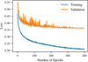 |
Fig. 5 Loss curves for the training process of the network. Loss values as a function of epoch are shown separately for training and validation data. |
5 Diagnostics
In this section, we quantify the reconstruction ability of our deep-learning model. The diagnostics will be performed in image space, which means that the reconstructed visibility distributions are processed by the inverse Fourier transformation before the evaluation techniques are applied on the reconstructed source distributions. Furthermore, we compare our deep-learning-based approach with the Cotton-Schwab clean algorithm (Schwab 1984) that is implemented in the established imaging software WSCLEAN (Offringa et al. 2014). Table 2 summarizes the cleaning parameters that we used for all cleaning tasks with WSCLEAN in this work. Due to the increasing complexity and computation times, we restricted ourselves to a small number of tuneable parameters. Therefore, we omitted the multiscale cleaning, for example, and used the conservative Cotton-Schwab clean algorithm. For both radionets and WSCLEAN, the goal is that the reconstructed and simulated radio galaxies do not deviate.
5.1 Comparison with WSCLEAN
As a first evaluation, we visually analyzed the visibility maps created with an inverse Fourier transform, shown in Fig. 6.
The corresponding source distributions in image space are shown in Fig. 7. In particular, we show the deep-learning-based source reconstruction, the simulated source distribution, and their difference. The mean values of the differences are an order of magnitude lower than the peak flux densities, meaning that simulation and prediction differ only slightly. Figure 8 shows the reconstruction for the same source using WSCLEAN. The comparison between the reconstructed and the simulated source distribution reveals a smeared-out source structure in the case of WSCLEAN. This smearing results from the convolution with the restoring beam inside the cleaning routine of WSCLEAN.
To test the model performance, we evaluated more than one image. To this end, we developed three diagnostic methods that focus on different aspects of a complete source reconstruc tion. We also used an existing evaluation metric, the multiscale structural similarity index measure (MS-SSIM), to compare the similarity between reconstructed and simulate source images. All four evaluation methods were applied to a distinctive test data set containing 10 000 images. The test images were the same for the radionets and the WSCLEAN evaluation.
First, we compared the reconstructed and simulated source areas. The necessary cut to distinguish source and background structures is 10% of the peak flux density. Then, the area of every source component in the image was computed and summed for the predicted and simulated source distribution. To do this, we obtained the contour levels using matplotlib and related them to the enclosed area using the Leibniz sector formula. A more detailed explanation can be found in our previous work (Schmidt et al. 2022). Figure 9 shows the area ratios for the radionets and the WSCLEAN reconstructions. The optimal value of one is reached when the source areas of the prediction and simulation are exactly the same. Ratios below one indicate an underestimated source area, while ratios above one denote over estimated areas. As shown in the histogram, reconstructed and simulated source areas match well in the case of radionets for most sources, which is confirmed by the mean ratio of 0.971 and the standard deviation of 0.088. In the case of WSCLEAN, the source area is overestimated by about 20% for most of the sources. The reason for this overestimate is the beam smearing in the WSCLEAN reconstruction routine. After creating a point-source model, the built model is convolved with the clean beam of the observation. This procedure spreads the source emission to a larger area on the sky. For a fair comparison between the radionets and WSCLEAN reconstruction, we took the smearing during our comparison with the simulated images into account. We used the clean beam computed by WSCLEAN to smear the simulated source distribution before we calculated the ratios for WSCLEAN.
The second method examines the peak flux densities of the predicted and simulated source distributions. Again, the above threshold is applied to define the source. Then, the ratio of the predicted and simulated peak flux densities was calculated. Figure 10 shows the values for the radionets and WSCLEAN reconstructions. The optimal ratio is again one, while ratios above and below indicate over- and underestimates, respectively. The distribution peaks around one, with a mean ratio of 0.998 and a standard deviation of 0.072 for radionets. This under lines that the brightest spot, for instance, the core of the source, is reconstructed well. Again, the comparison with WSCLEAN is slightly more complicated. Beam-smearing effects have to be taken into account before the peak flux density can be compared with the simulated source distribution. While the simulated flux densities are in units of Jy px−1, the WSCLEAN reconstructions are in units of Jy beam−1. We computed the beam area, divided it by the pixel area, and used the scaling factor to scale the flux densi ties of the WSCLEAN images so that they matched the simulations.
To calculate the beam area, we used the expression
 (9)
(9)
where bmin is the full width at half maximum (FWHM) of the minor axis of the beam, and bmaj is the FWHM of the major axis of the beam. Even though the images have the same flux den sity units, the peak flux density of the WSCLEAN reconstruction is underestimated by a factor of two, with a mean ratio of 0.481 and a standard deviation of 0.059. The beam smears the initial peak flux to neighboring pixels, which causes a decrease in the peak flux density in this individual pixel. Another effect that must be taken into account is that the effective resolution for radionets is higher than for WSCLEAN, as can be seen in the right images of Figs. 7 and 8. Thus, the beam smearing that cannot be corrected for and the difference in resolution lead to the expected lower peak flux densities for WSCLEAN.
For the third diagnostic method, we summed all flux densi ties inside of the 10% peak flux density threshold to calculate the integrated flux density. Then, we computed the ratio of the values for reconstruction and simulation. Figure 11 shows the result ing ratios for WSCLEAN and radionets. For both reconstruction techniques, the integrated peak flux densities match well for the complete test data set. The good agreement is apparent in the mean and standard deviation of 0.976 ± 0.053 for radionets and 0.975 ± 0.069 for WSCLEAN. In the case of the integrated flux density, the beam smearing of WSCLEAN plays no longer a significant role after the images are transformed from units of Jy beam−1 into units of Jy px−1.
For a more image-based comparison of the simulated and the predicted source distributions, we used a criterion that is com monly used in the field of computer vision, the MS-SSIM (Wang et al. 2003). This metric is split into three distinctive parts, which are luminance, contrast, and structure:
 (10)
(10)
 (11)
(11)
 (12)
(12)
with μ as the mean, σ as the standard deviation, σху as the covariance, x and y as the images to be compared, and
 (13)
(13)
Here, L refers to the dynamic range of the pixel values, and K1 ≪ 1 and K2 ≪ 1 are small scalar constants that are used to correct for numerical instabilities in the denominator. The metric is then a combination of the three components (10) to (12),
![Mathematical equation: ${\rm{SSIM}}\left( {x,y} \right) = {\left[ {{l_M}\left( {x,y} \right)} \right]^{{\alpha _M}}}\prod\limits_{j = 1}^M {{{\left[ {{c_j}\left( {x,y} \right)} \right]}^{{\beta _j}}}{{\left[ {{s_j}\left( {x,y} \right)} \right]}^{{\gamma _j}}}} .$](/articles/aa/full_html/2023/09/aa47073-23/aa47073-23-eq15.png) (14)
(14)
This formula is an improvement over the predecessor because it opens up the possibility to use image details at different resolu tions. The optimal value is one, which can only be achieved if x = y.
As in the previous three evaluation methods, we recon structed 10 000 test sources with WSCLEAN and radionets. Then, we computed the MS-SSIM between the reconstructed and simulated source distributions (see Fig. 12). In the case of radionets, the distribution peaks around the optimal value of one. Further evidence for the good performance is the fact that the mean is 0.999 and the standard deviation is 0.002. In terms of computer-vision and image-reconstruction tasks, the predicted and simulated source distributions are very similar, with very few outliers. This proves that our approach is robust and can model the noisy input images and more complex source struc tures, which is a major improvement over the Gaussian sources from our previous work. For WSCLEAN, the results are worse, with a mean and standard deviation of 0.920 ± 0.062. The effect is related to the beam smearing inside the cleaning routine in WSCLEAN. The deviation of the MS-SSIM is consistent with the distributions shown in Fig. 9. Even though we applied the same clean beam to the simulated sources before calculating the MS-SSIM, the beam-smearing effects cannot be completely cor rected for, which results in a source area overestimation of about 20%. When computing the mean structural similarities, this area overestimation leads to deviations from the optimal value of one in the case of WSCLEAN. All mean values and standard deviations from the four methods are summarized in Table 3.
In order to test the robustness of both approaches, we split the results of the evaluation methods into the different S/Ns of the input data. The S/Ns of the input data were quantified with the help of WSCLEAN. We ran WSCLEAN on the test data with the settings summarized in Table 2, but the auto-mask option was set to 5. We then calculated the S/N as follows:
 (15)
(15)
Here, Iclean denotes the clean image, and Iresidual represents the residual image. The resulting S/N distribution is shown in Fig. H.1. Figure H.2 shows input data with an S/N of 5, 35, and 70 for a visual analysis of the different noise levels.
We created seven S/N categories, 0–10, 10–20, and so on, with the final category being all S/Ns above 60. To compare radionets and WSCLEAN, we computed the mean and standard deviation for each category, and we plot the standard deviation against the mean ratio.
Figure 13 shows the means and standard deviations of the area ratios from Fig. 9 split into the different S/Ns of the input visibility maps. Both reconstruction techniques converge to the optimal mean ratio of one and the optimal standard deviation of zero for larger S/Ns. While radionets reconstructions underes timate the source areas for smaller S/Ns, WSCLEAN overestimates the source areas for these cases.
The means and standard deviations of the peak flux den sity ratios from Fig. 10 are shown in Fig. 14. The analysis of the results for the different S/Ns of the input visibilities reveals no significant improvements in the mean ratios. The standard deviation is slightly improved with increasing S/N. Peak flux densities for WSCLEAN are underestimated too much because no exact correction for the beam smearing to neighboring pixels is possible.
In Fig. 15, we show the mean and standard deviations for the integrated flux density ratios. A significant improvement for means and standard deviations is evident for radionets and WSCLEAN reconstructions. For both reconstruction techniques, the highest S/Ns converge to the optimal mean of one and the optimal standard deviation of zero.
Figure 16 shows the mean and standard deviation of the MS-SSIM split into the different S/Ns of the input visibilities. For the radionets reconstructions, the MS-SSIM does not sig nificantly change for different S/Ns, while the results improve with higher S/Ns in the case of WSCLEAN. The lower MS-SSIM values for WSCLEAN originate from the smeared-out source structures because of the clean beam of the observation. The clean beam improves with higher S/Ns. Consequently, the smearing decreases, which results in an improved MS-SSIM. A detailed summary of the corresponding values is given in Table G.1 for radionets and in Table G.2 for WSCLEAN.
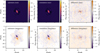 |
Fig. 6 Exemplary reconstruction in Fourier space for the deep-learning-based cleaning approach. We show the prediction (left), the true distribution (middle), and the difference between the two (right). Results are shown for the real (top) and imaginary (bottom) part. |
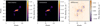 |
Fig. 7 Image space reconstruction for the deep-learning-based cleaning approach. We show the predicted source distribution (left), the simulated source distribution (middle), and the difference between the two (right). The real and imaginary visibility maps used for the inverse Fourier transformation are those shown in Fig. 6. |
Overview of the parameter settings used to create the clean images using WSCLEAN.
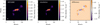 |
Fig. 8 Clean image generated using WSCLEAN. Reconstructed clean image (left), simulated source distribution (middle), and difference between reconstruction and simulation (right). The WSCLEAN reconstruction was converted into units of Jy · px−1 for comparability with the simulations. For the clean image generated by WSCLEAN, the clean beam is shown at the lower left edge. |
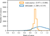 |
Fig. 9 Ratio of the true and predicted areas for the radionets and WSCLEAN reconstructions. For both reconstruction approaches, the mean and standard deviation is given. In the case of WSCLEAN, the area ratio is corrected for the beam smearing. |
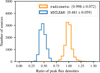 |
Fig. 10 Ratio of the true and predicted peak flux densities for the radionets and WSCLEAN reconstructions. For both reconstruction approaches, the mean and standard deviation is given. In the case of WSCLEAN, the flux density is converted from units of Jy beam−1 into Jy px−1. The obvious difference between the distributions originates from different effective resolutions that the methods can achieve. |
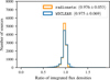 |
Fig. 11 Ratio of the true and predicted integrated flux densities for the radionets and WSCLEAN reconstructions. For both reconstruction approaches, the mean and standard deviation is given. In the case of WSCLEAN, the flux density is converted from units of Jy beam−1 into Jy px−1. |
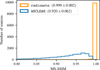 |
Fig. 12 MS-SSIM for the radionets and WSCLEAN reconstructions. For both reconstruction approaches, the mean and standard deviation is given. For a fair comparison of the source structures, the true source dis tributions are smeared out with the clean beam calculated by WSCLEAN. |
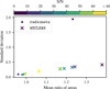 |
Fig. 13 Means and standard deviations of the area ratios from Fig. 9 split into the different S/Ns of the input visibility maps. Results are shown for the radionets and WSCLEAN reconstructions. |
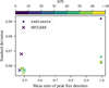 |
Fig. 14 Means and standard deviations of the peak flux density ratios from Fig. 10 split into the different S/Ns of the input visibility maps. Results are shown for radionets and WSCLEAN reconstructions. |
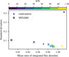 |
Fig. 15 Means and standard deviations of the integrated flux density ratios from Fig. 11 split into the different S/Ns of the input visibility maps. Results are shown for radionets and WSCLEAN reconstructions. |
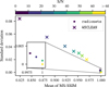 |
Fig. 16 Means and standard deviations of the MS-SSIM from Fig. 12 split into the different S/Ns of the input visibility maps. Results are shown for radionets and WSCLEAN reconstructions. |
Comparison of runtimes to reconstruct simulated observations with WSCLEAN and radionets.
5.2 Computing times
A major advantage of the deep-learning-based analysis are the short computing times after the deep-learning model was trained. While WSCLEAN requires around 4.5 s to process a 128 px × 128 px simulation, our radionets framework needed less than half this time, with 2.01 s (DL reco + I/O). This reconstruction time also includes data operations such as data loading, model loading, and saving the reconstruction. Data operations are expected to be accelerated in the future because they are not yet optimized. The pure reconstruction times for the deep-learning model (DL reco) are even faster because convolutional neural networks (CNN) are very efficient when applied to image data. The neural network models need about 40 ms to reconstruct a 128 px × 128 px simulation. All computing times are summarized in Table 4.
6 Future work
We have demonstrated the potential of radio interferometric imaging using deep-learning techniques. Some work still needs to be done until this technique can be applied to real data. In particular, we focus on two issues that we discuss below.
6.1 Uncertainty estimates
Our neural network should not only reconstruct images, but also estimate their uncertainty. The uncertainty can be estimated by using a negative log likelihood lß-NLL as loss function, following Valdenegro-Toro & Saromo-Mori (2022) and The IceCube Collaboration (2021),
 (16)
(16)
 (17)
(17)
Now, a Gaussian distribution is predicted for each pixel. The neural network model introduced in Sect. 4 served to predict the mean values, while a second convolutional network was used to predict the variances. Sampling from these Gaussian distributions quantifies the uncertainties in Fourier and in image space.
Hence, we are able to estimate the reconstruction error of source types on which the neural network has not been trained. This can be illustrated with the example of an image of a cat (see Fig. 17, right). First, we simulated the observation of the cat with the mask in Fourier space used above. The gridded visibilities were then evaluated with our model, which was trained on the FIRST simulations, as explained in Sect. 2 and Sect. 3. Then we were able to create the mean reconstruction as well as the corresponding uncertainty map (see Fig. 17). It appears that the network is able to reconstruct parts of the left eye of the cat, but not much more because it has been trained on images with a completely different shape. Consequently, the uncertainty map highlights exactly the areas that are reconstructed. This means that the network is uncertain with its prediction, which is the expected behavior. This feature could help to detect unknown source shapes.
Additionally, we tested our uncertainty approach on source distributions from the test data set introduced in Sect. 5. Figure 18 visualizes the reconstruction and the corresponding uncertainty map. Simulated source distribution (upper left) and deep-learning reconstruction (upper right) agree well. When the difference map (lower right) between simulation and prediction is computed, two problems become apparent. The point source below the main part of the radio source is not reconstructed in the prediction of the neural network. Simultaneously, the prediction shows a feature above the central radio source, which is an artifact in the reconstruction. Both features are represented in the calculated uncertainty map (lower left). Especially for the missing point source, the intensity inside the uncertainty map is not high enough to cover the difference between simulation and prediction. For the central source structure, the uncertainty map covers the deviation between simulation and prediction because it is significantly lower. In our future work, we will focus on improving the coverage of the actual difference for the uncertainty maps.
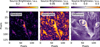 |
Fig. 17 Overview of the prediction (left) and uncertainty (right) maps of an image of a cat. Image is taken from Scikit-image: Chelsea the cat, by Stefan van der Walt. |
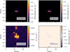 |
Fig. 18 Reconstruction and uncertainty map of a radio galaxy from the test data set. While the shown source reconstruction (upper right) is generated by calculating the mean of the sampled reconstructions, their standard deviation gives the uncertainty map (lower left). Simulated source distribution (upper left) and prediction agree well, which is reflected by their difference map (lower right). |
6.2 Wide-field and survey data
Modern radio interferometers have wide fields of view and record multifrequency data. In future work, we will focus on enhancing our simulation chain to take these specifications into account. One approach to improve the simulations to match sky survey data is to choose larger sky sections as input for the RIME formalism. In addition to the central main source, we will simulate other sources around the pointing center of the simulated observation. Thus, noise from bright neighboring sources will be taken into account in the visibility data.
In order to improve the deep-learning-based imaging, we plan to exploit the spectral data of different frequency channels. Because data do not vary strongly between neighboring channels, the reconstruction of the first channel constitutes a good initial guess for the reconstruction of the second channel. Processing this information inside the deep-learning model has the potential to significantly improve and speed up the reconstruction of data cubes.
Furthermore, the reconstruction can be improved even more by enhancing the gridder. Currently, our gridder creates a simple two-dimensional histogram, as explained in Sect. 3. This approach is different from established gridders, which use convolutional gridding to facilitate subsequent imaging. Especially in connection with the large fields of view of modern sky surveys, wide-field gridding methods will also be relevant for imaging with deep-learning techniques.
7 Conclusions
We have focused on improving the training data for our neural network. To this end, we produced realistic radio galaxy simulations and modeled the measurement process of a radio interferometer.
Our image simulation was based on the GAN developed in Kummer et al. (2022); Rustige et al. (2023). The GAN can produce an arbitrary number of realistic images of radio galaxies that resemble images from the FIRST survey.
These radio sources were then used as input for the RIME formalism presented in Sect. 3. We considered the phase delay and the antenna characteristics for the simulation process and also smeared the simulated measurement with noise originating from the measurement process. Various parameters for a real measurement were also taken into account, such as the coordinates of the center of the FOV randomly, as shown in Table 1.
The GAN-generated radio galaxies were processed through the RIME framework and then used as input for our neural network. The main neural network was the same as in Schmidt et al. (2022) with small adjustments, such as twice the number of residual blocks. The training process ran smoothly, as shown in Fig. 5, and produced reconstructions that matched the corresponding simulated sky simulation very well, as shown in Fig. 6.
To generalize the performance of the trained model, we evaluated the sources in image space using three methods that compared area, peak flux density, and integrated flux density. This was supplemented by a method adopted from the field of computer vision, which is called MS-SSIM. Each of these methods was applied to 10 000 reconstructions from radionets and from WSCLEAN. The results are shown in Fig. 9 to Fig. 12. While for the ratio of integrated flux densities, radionets and WSCLEAN performed equally well, WSCLEAN overestimated and underestimated the areas and the MS-SSIM, respectively. The results for the peak flux densities for both methods varied widely due to resolution differences, as shown in the comparison of the right images in Figs. 7 and 8. Overall, radionets was able to reconstruct far more complex source structures than in our previous paper and needed only minor adjustments. It also performed at least as well as WSCLEAN for the main source properties. However, due to non-correctable beam-smearing effects and different effective resolutions, the comparison is not entirely fair.
Then, we divided the results according to their S/N. The expectation was that for images with a high S/N, the mean and standard deviations of our diagnostic methods would be closer to their respective optimal values than for images with a lower S/N. This applies to both radionets and WSCLEAN. Figures 13–16 show that this expectation holds in almost every case, except for the peak flux densities, for which the results are very similar for every S/N except for S/N 10. Thus, our network is robust and able to reconstruct complex structures even though the S/N is rather low.
To summarize, we improved our simulations with two key features: (i) the GAN-generated radio galaxy images, and (ii) the simulation of an interferometer measurement using RIME. With these two developments, we are able to train our network with more realistic data. As a result, the network is able to reconstruct the sources with similar accuracy as WSCLEAN, despite the increased complexity of the sources. Finally, the evaluation metrics suggest a better performance than the model in Schmidt et al. (2022). The two frameworks, pyvisgen (Schmidt et al. 2020) for the simulation part and radionets (Schmidt et al. 2023) for the model training, are available on GitHub.
Finally, we give an outlook on future features of our deep-learning-based approach. We focus on estimating the reconstruction error, as outlined in Fig. 17, by extending the neural network such that it computes uncertainties as well as visibility reconstructions. The second goal is the application of our deep-learning-based imaging approach to actual observation data. In the future, we will focus on the minimization of data-simulation mismatches to train deep-learning models that are suitable for reconstructing survey data of large parts of the sky.
Acknowledgments
M.B. acknowledges support from the Deutsche Forschungsgemeinschaft (DFG) under Germany’s Excellence Strategy - EXC 2121 “Quantum Universe” - 390833306, funding through the DFG Research Unit FOR 5195 and via the KISS consortium (05D23GU4, 13D22CH5) funded by the German Federal Ministry of Education and Research BMBF in the ErUM-Data action plan. The authors acknowledge support from the project “Big Bang to Big Data (B3D)”. B3D is receiving funding from the program “Profilbildung 2020”, an initiative of the Ministry of Culture and Science of the State of North Rhine- Westphalia. The sole responsibility for the content of this publication lies with the authors. D.E. acknowledges funding through the BMBF for the reasearch project D-MeerKAT-II and D-MeerKAT-III in the ErUM-Data context. The authors acknowledge support from the German Science Foundation (DFG) within the Collaborative Research Center SFB1491. We thank the anonymous referee for an insightful and stimulating report.
Appendix A Software and packages
We used PyTorch (Paszke et al. 2019) as the fundamental deep-learning framework. It was chosen because of its flexibility and the ability to directly develop algorithms in the programming language Python (Python Software Foundation 20202). In addition to PyTorch, we used the deep-learning library fast.ai (Howard et al. 2018), which supplies high-level components to build customized deep-learning algorithms in a quick and efficient way. For simulations and data analysis, the Python packages NumPy (Oliphant 2006), Astropy (Astropy Collaboration 2013, 2018), Cartopy (Met Office 2011-20183), scikit-image (Van der Walt et al. 2014), and Pandas (McKinney et al. 2010) were used. The results were illustrated using the plotting package Matplotlib (Hunter 2007). A full list of the packages and our developed open-source radionets framework can be found on github4. More information about our developed open-source simulation framework pyvisgen can be found in the git repository5.
Appendix B Gaussian smoothing of GAN-generated radio galaxies
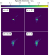 |
Fig. B.1 Effect of a Gaussian filter on the GAN-generated sources. We decided to use a smoothing of σ = 0.75 px due to the best effect without creating false point sources, as visible for σ = 1 px. |
Appendix C Phase versus imaginary part
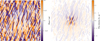 |
Fig. C.1 Fourier-transformed source with the corresponding phase part (left) and imaginary part (right). The structures in the center of the images are very similar, but the edges differ, especially in terms of intensity. |
Appendix D Computer setup
Computer specifications for the setup used in the training process
Appendix E Antenna positions in VLA B-configuration
Overview of the antenna positions of the VLA used for the RIME in the Earth-centered coordinate system. The positions correspond to the B-configuration of the VLA used for the FIRST observations.
Appendix F Visualization of Jones matrices
 |
Fig. F.1 Visualization of Jones K(l, m), which represents the phase-delay effect. Examples are given for three different antenna pairs of the VLA. |
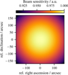 |
Fig. F.2 Visualization of Jones E(l, m), which represents the telescope beam effects. |
Appendix G Summary of the results of the evaluation methods
Results of the evaluation methods for data sets with different S/Ns reconstructed with radionets
Results of the evaluation methods for data sets with different S/Ns reconstructed with WSCLEAN
Appendix H Signal-to-noise ratios
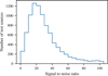 |
Fig. H.1 Overview of the S/Ns of the sources inside the test data set. The majority of the sources have an S/N between 10 and 40. |
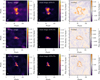 |
Fig.H.2 WSCLEAN results for simulations with different S/Ns. A dirty image (left), clean image (middle), and remaining residual (right) are shown for an S/N of 5 (top), 35 (middle), and 70 (bottom). |
References
- Amari, S.-I. 1993, Neurocomputing, 5, 185 [CrossRef] [Google Scholar]
- Arjovsky, M., Chintala, S., & Bottou, L. 2017, ArXiv e-prints [arXiv:1701.07875] [Google Scholar]
- Astropy Collaboration (Robitaille, T.P., et al.) 2013, A&A, 558, A33 [NASA ADS] [CrossRef] [EDP Sciences] [Google Scholar]
- Astropy Collaboration (Price-Whelan, A.M., et al.) 2018, AJ, 156, 123 [NASA ADS] [CrossRef] [Google Scholar]
- Becker, R.H., White, R.L., & Helfand, D.J. 1995, ApJ, 450, 559 [NASA ADS] [CrossRef] [Google Scholar]
- Clark, B.G. 1980, A&A, 89, 377 [NASA ADS] [Google Scholar]
- Delli Veneri, M., Tychoniec, L., Guglielmetti, F., Longo, G., & Villard, E. 2022, MNRAS, 518, 3407 [CrossRef] [Google Scholar]
- Fanaroff, B.L., & Riley, J.M. 1974, MNRAS, 167, 31 [Google Scholar]
- Goodfellow, I.J., Pouget-Abadie, J., Mirza, M., et al. 2014, ArXiv e-prints [arXiv:1406.2661] [Google Scholar]
- Goodfellow, I., Bengio, Y., & Courville, A. 2016, Deep Learning – Chapter 9: Convolutional Networks (MIT Press) [Google Scholar]
- Grainge, K., Alachkar, B., Amy, S., et al. 2017, Astron. Rep., 61, 288 [NASA ADS] [CrossRef] [Google Scholar]
- Griese, F., Kummer, J., & Rustige, L. 2022, https://doi.org/10.5281/zenodo.7120632 [Google Scholar]
- Griese, F., Kummer, J., Connor, P.L.S., Bruggen, M., & Rustige, L. 2023, Data in Brief, 47, 108974 [NASA ADS] [CrossRef] [Google Scholar]
- Gross, S., & Wilber, M. 2016, Training and investigating Residual Nets [Google Scholar]
- Hamaker, J.P., Bregman, J.D., & Sault, R.J. 1996, A&AS, 117, 137 [NASA ADS] [CrossRef] [EDP Sciences] [Google Scholar]
- He, K., Zhang, X., Ren, S., & Sun, J. 2015, ArXiv e-prints [arXiv:1512.03385] [Google Scholar]
- Howard, J., et al. 2018, https://github.com/fastai/fastai [Google Scholar]
- Hunter, J.D. 2007, Comput. Sci. Eng., 9, 90 [Google Scholar]
- Kingma, D.P., & Ba, J. 2014, ArXiv e-prints [arXiv:1412.6980] [Google Scholar]
- Kummer, J., Rustige, L., Griese, F., et al. 2022, in INFORMATIK 2022, Lecture Notes in Informatics (LNI) — Proceedings, P-326 (Bonn: Gesellschaft fur Informatik), 469 [Google Scholar]
- Ledig, C., Theis, L., Huszar, F., et al. 2016, ArXiv e-prints [arXiv:1609.04802] [Google Scholar]
- McKinney, W. et al. 2010, in Proceedings of the 9th Python in Science Conference, 445, 51 [Google Scholar]
- Medeiros, L., Psaltis, D., Lauer, T.R., & Ozel, F. 2023, ApJ, 947, L7 [NASA ADS] [CrossRef] [Google Scholar]
- NRAO 2023, Sensitivity, https://science.nrao.edu/facilities/vla/docs/manuals/oss/performance/sensitivity [Google Scholar]
- Offringa, A.R., McKinley, B., Hurley-Walker, N., et al. 2014, MNRAS, 444, 606 [NASA ADS] [CrossRef] [Google Scholar]
- Oliphant, T.E. 2006, A Guide to NumPy, 1 (USA: Trelgol Publishing) [Google Scholar]
- Paszke, A., Gross, S., Massa, F., et al. 2019, in Advances in Neural Information Processing Systems, 32, eds. H. Wallach, H. Larochelle, A. Beygelzimer, F. Alche-Buc, E. Fox, & R. Garnett (Curran Associates, Inc.), 8026 [Google Scholar]
- Rustige, L., Kummer, J., Griese, F., et al. 2023, RAS Techniques and Instruments, 2, 264 [NASA ADS] [CrossRef] [Google Scholar]
- Salimans, T., Goodfellow, I., Zaremba, W., et al. 2016, ArXiv e-prints [arXiv:1606.03498] [Google Scholar]
- Schmidt, K., Geyer, F., et al. 2020, https://github.com/radionets-project/pyvisgen [Google Scholar]
- Schmidt, K., Geyer, F., Frose, S., et al. 2022, A&A, 664, A134 [NASA ADS] [CrossRef] [EDP Sciences] [Google Scholar]
- Schmidt, K., Geyer, F., Poggenpohl, A., & Elsasser, D. 2023, https://github.com/radionets-project/radionets [Google Scholar]
- Schwab, F.R. 1984, AJ, 89, 1076 [NASA ADS] [CrossRef] [Google Scholar]
- Smirnov, O.M. 2011, A&A, 527, A106 [NASA ADS] [CrossRef] [EDP Sciences] [Google Scholar]
- Taylor, G.B., Carilli, C.L., & Perley, R.A. 1999, ASP Conf. Ser., 180 [Google Scholar]
- The CASA Team, Bean, B., Bhatnagar, S., et al. 2022, PASP, 134, 114501 [NASA ADS] [CrossRef] [Google Scholar]
- The IceCube Collaboration 2021, J. Instrum., 16, P07041 [CrossRef] [Google Scholar]
- Valdenegro-Toro, M., & Saromo-Mori, D. 2022, in 2022 IEEE/CVF Conference on Computer Vision and Pattern Recognition Workshops (CVPRW), 1508 [CrossRef] [Google Scholar]
- Van derWalt, S., Schonberger, J.L., Nunez-Iglesias, J., et al. 2014, PeerJ, 2, e453 [CrossRef] [PubMed] [Google Scholar]
- van Haarlem, M.P., Wise, M.W., Gunst, A.W., et al. 2013, A&A, 556, A2 [NASA ADS] [CrossRef] [EDP Sciences] [Google Scholar]
- Wang, Z., Simoncelli, E., & Bovik, A. 2003, in The Thirty-Seventh Asilomar Conference on Signals, Systems & Computers, 2003, 2, 1398 [Google Scholar]
All Tables
Overview of the parameter settings used to create the clean images using WSCLEAN.
Comparison of runtimes to reconstruct simulated observations with WSCLEAN and radionets.
Overview of the antenna positions of the VLA used for the RIME in the Earth-centered coordinate system. The positions correspond to the B-configuration of the VLA used for the FIRST observations.
Results of the evaluation methods for data sets with different S/Ns reconstructed with radionets
Results of the evaluation methods for data sets with different S/Ns reconstructed with WSCLEAN
All Figures
|
Fig. 1 Analysis chain used in this work. The analysis chain handles data in image space (green) and Fourier space (orange). It is structured in three parts: simulations, neural network model, and evaluation. |
| In the text | |
|
Fig. 2 Schematics of the wGAN architecture reproduced from Rustige et al. (2023), where y denotes the class label of real x or generated images |
| In the text | |
|
Fig. 3 Exemplary (u, v) coverage of a VLA simulation using the developed RIME implementation. |
| In the text | |
|
Fig. 4 Overview of the training routine. |
| In the text | |
|
Fig. 5 Loss curves for the training process of the network. Loss values as a function of epoch are shown separately for training and validation data. |
| In the text | |
|
Fig. 6 Exemplary reconstruction in Fourier space for the deep-learning-based cleaning approach. We show the prediction (left), the true distribution (middle), and the difference between the two (right). Results are shown for the real (top) and imaginary (bottom) part. |
| In the text | |
|
Fig. 7 Image space reconstruction for the deep-learning-based cleaning approach. We show the predicted source distribution (left), the simulated source distribution (middle), and the difference between the two (right). The real and imaginary visibility maps used for the inverse Fourier transformation are those shown in Fig. 6. |
| In the text | |
|
Fig. 8 Clean image generated using WSCLEAN. Reconstructed clean image (left), simulated source distribution (middle), and difference between reconstruction and simulation (right). The WSCLEAN reconstruction was converted into units of Jy · px−1 for comparability with the simulations. For the clean image generated by WSCLEAN, the clean beam is shown at the lower left edge. |
| In the text | |
|
Fig. 9 Ratio of the true and predicted areas for the radionets and WSCLEAN reconstructions. For both reconstruction approaches, the mean and standard deviation is given. In the case of WSCLEAN, the area ratio is corrected for the beam smearing. |
| In the text | |
|
Fig. 10 Ratio of the true and predicted peak flux densities for the radionets and WSCLEAN reconstructions. For both reconstruction approaches, the mean and standard deviation is given. In the case of WSCLEAN, the flux density is converted from units of Jy beam−1 into Jy px−1. The obvious difference between the distributions originates from different effective resolutions that the methods can achieve. |
| In the text | |
|
Fig. 11 Ratio of the true and predicted integrated flux densities for the radionets and WSCLEAN reconstructions. For both reconstruction approaches, the mean and standard deviation is given. In the case of WSCLEAN, the flux density is converted from units of Jy beam−1 into Jy px−1. |
| In the text | |
|
Fig. 12 MS-SSIM for the radionets and WSCLEAN reconstructions. For both reconstruction approaches, the mean and standard deviation is given. For a fair comparison of the source structures, the true source dis tributions are smeared out with the clean beam calculated by WSCLEAN. |
| In the text | |
|
Fig. 13 Means and standard deviations of the area ratios from Fig. 9 split into the different S/Ns of the input visibility maps. Results are shown for the radionets and WSCLEAN reconstructions. |
| In the text | |
|
Fig. 14 Means and standard deviations of the peak flux density ratios from Fig. 10 split into the different S/Ns of the input visibility maps. Results are shown for radionets and WSCLEAN reconstructions. |
| In the text | |
|
Fig. 15 Means and standard deviations of the integrated flux density ratios from Fig. 11 split into the different S/Ns of the input visibility maps. Results are shown for radionets and WSCLEAN reconstructions. |
| In the text | |
|
Fig. 16 Means and standard deviations of the MS-SSIM from Fig. 12 split into the different S/Ns of the input visibility maps. Results are shown for radionets and WSCLEAN reconstructions. |
| In the text | |
|
Fig. 17 Overview of the prediction (left) and uncertainty (right) maps of an image of a cat. Image is taken from Scikit-image: Chelsea the cat, by Stefan van der Walt. |
| In the text | |
|
Fig. 18 Reconstruction and uncertainty map of a radio galaxy from the test data set. While the shown source reconstruction (upper right) is generated by calculating the mean of the sampled reconstructions, their standard deviation gives the uncertainty map (lower left). Simulated source distribution (upper left) and prediction agree well, which is reflected by their difference map (lower right). |
| In the text | |
|
Fig. B.1 Effect of a Gaussian filter on the GAN-generated sources. We decided to use a smoothing of σ = 0.75 px due to the best effect without creating false point sources, as visible for σ = 1 px. |
| In the text | |
|
Fig. C.1 Fourier-transformed source with the corresponding phase part (left) and imaginary part (right). The structures in the center of the images are very similar, but the edges differ, especially in terms of intensity. |
| In the text | |
|
Fig. F.1 Visualization of Jones K(l, m), which represents the phase-delay effect. Examples are given for three different antenna pairs of the VLA. |
| In the text | |
|
Fig. F.2 Visualization of Jones E(l, m), which represents the telescope beam effects. |
| In the text | |
|
Fig. H.1 Overview of the S/Ns of the sources inside the test data set. The majority of the sources have an S/N between 10 and 40. |
| In the text | |
|
Fig.H.2 WSCLEAN results for simulations with different S/Ns. A dirty image (left), clean image (middle), and remaining residual (right) are shown for an S/N of 5 (top), 35 (middle), and 70 (bottom). |
| In the text | |
Current usage metrics show cumulative count of Article Views (full-text article views including HTML views, PDF and ePub downloads, according to the available data) and Abstracts Views on Vision4Press platform.
Data correspond to usage on the plateform after 2015. The current usage metrics is available 48-96 hours after online publication and is updated daily on week days.
Initial download of the metrics may take a while.