| Issue |
A&A
Volume 677, September 2023
|
|
|---|---|---|
| Article Number | A144 | |
| Number of page(s) | 16 | |
| Section | Catalogs and data | |
| DOI | https://doi.org/10.1051/0004-6361/202346778 | |
| Published online | 19 September 2023 | |
The RoboPol sample of optical polarimetric standards★
1
Institute of Astrophysics, Foundation for Research and Technology-Hellas,
N. Plastira 100, Vassilika Vouton,
71110
Heraklion, Greece
e-mail: This email address is being protected from spambots. You need JavaScript enabled to view it.
2
Department of Physics, and Institute for Theoretical and Computational Physics, University of Crete, Voutes University campus,
70013
Heraklion, Greece
3
South African Astronomical Observatory,
PO Box 9,
Observatory,
7935
Cape Town, South Africa
4
Inter-University Centre for Astronomy and Astrophysics,
Post Bag 4,
Ganeshkhind,
Pune-411007, India
5
Institute of Theoretical Astrophysics, University of Oslo,
PO Box 1029
Blindern,
0315
Oslo, Norway
6
Finnish Centre for Astronomy with ESO, FINCA, University of Turku, Quantum,
Vesilinnantie 5,
20014
Turku, Finland
7
Department of Physics and Astronomy, University of Turku,
20014
Turku, Finland
8
Department of Space, Earth and Environment, Chalmers University of Technology,
Gothenburg, Sweden
9
University of California, Los Angeles, Geophysics and Space Physics Department of Earth, Planetary, and Space Sciences,
Los Angeles, USA
10
Owens Valley Radio Observatory, California Institute of Technology,
MC 249-17,
Pasadena, CA
91125, USA
11
Department of Astronomy/Steward Observatory,
Tucson, AZ
85721-0065, USA
12
Section of Astrophysics, Astronomy & Mechanics, Department of Physics, National and Kapodistrian University of Athens,
Panepistimiopolis Zografos
15784, Greece
13
Department of Physics, Gauhati University,
Guwahati -
781014,
Assam,
India
14
Institute of Astronomy, Faculty of Physics, Astronomy and Informatics, Nicolaus Copernicus University in Toruń,
Grudziadzka 5,
87-100
Toruń, Poland
15
Cahill Center for Astronomy and Astrophysics, California Institute of Technology,
1200 E California Blvd,
MC 249-17,
Pasadena, CA
91125, USA
16
Institut de Radioastronomie Millimétrique,
Avenida Divina Pastora 7, Local 20,
18012
Granada, Spain
17
Max-Planck-Institut für Radioastronomie,
Auf dem Hügel 69,
53121
Bonn, Germany
18
Department of Physics, University of Johannesburg,
PO Box 524,
Auckland Park
2006, South Africa
19
Joint Institute for VLBI ERIC,
Oude Hoogevceensedijk 4,
7991 PD
Dwingeloo, The Netherlands
Received:
29
April
2023
Accepted:
19
July
2023
Abstract
Context. Optical polarimeters are typically calibrated using measurements of stars with known and stable polarization parameters. However, there is a lack of such stars available across the sky. Many of the currently available standards are not suitable for medium and large telescopes due to their high brightness. Moreover, as we find, some of the polarimetric standards used are in fact variable or have polarization parameters that differ from their cataloged values.
Aims. Our goal is to establish a sample of stable standards suitable for calibrating linear optical polarimeters with an accuracy down to 10−3 in fractional polarization.
Methods. For 4 yr, we have been running a monitoring campaign of a sample of standard candidates comprised of 107 stars distributed across the northern sky. We analyzed the variability of the linear polarization of these stars, taking into account the non-Gaussian nature of fractional polarization measurements. For a subsample of nine stars, we also performed multiband polarization measurements.
Results. We created a new catalog of 65 stars (see Table 2) that are stable, have small uncertainties of measured polarimetric parameters, and can be used as calibrators of polarimeters at medium and large telescopes.
Key words: polarization / techniques: polarimetric / standards
All data discussed in this paper are available in Harvard Dataverse at https://doi.org/10.7910/DVN/IV9TXX.
© The Authors 2023
 Open Access article, published by EDP Sciences, under the terms of the Creative Commons Attribution License (https://creativecommons.org/licenses/by/4.0), which permits unrestricted use, distribution, and reproduction in any medium, provided the original work is properly cited.
This article is published in open access under the Subscribe to Open model. This email address is being protected from spambots. You need JavaScript enabled to view it. to support open access publication.
1 Introduction
Polarimetry, on its own and in combination with other techniques, is a powerful tool for probing the physical conditions of astrophysical sources. Like all experimental techniques, polari-metric observations require careful calibration and control of instrumental systematics. In the case of optical polarimetry, standard stars with known polarization properties are used for calibration purposes. Unfortunately, the number of reliable polarimetric standards is very limited. There are fewer than 30 stars in the two hemispheres with polarization degree (PD) known to an accuracy of 0.1% or better, and proven to be stable in time (e.g., Schmidt et al. 1992; Hsu & Breger 1982). The lack of an appropriate unpolarized standard star in the night sky at a given moment is common.
The situation is particularly difficult for telescopes with apertures larger than 1m. They often have a lower limit on the brightness of sources suitable for observations due to CCD saturation constraints. Meanwhile, most unpolarized standards are very bright (<8m), making them unsuitable for calibration on such telescopes because unpolarized standards are selected from nearby stars to ensure that their light does not pass through a significant column of dust in the interstellar medium.
Another problem is the lack of polarized standards with low, but not negligible, PD in the range between 0.1 and 2%. Existing measurements of standards with PD > 2% have been sufficient to calibrate conventional polarimeters, and there has been no need for covering a lower range of PD. It is because conventional polarimeters have (or are assumed to have) negligible crosstalk between the Stokes parameters, meaning that the parameters are independent and uncorrelated. In this case we use unpolarized stars (zero-polarized or negligibly polarized) to find the offset of the instrumental Q/I–U/I plane with respect to the standard value and (2) highly polarized stars to find a rotation of the instrumental relative Stokes parameters plane with respect to the standard value (e.g., Ramaprakash et al. 2019). However, some new polarimeters have significant crosstalk (Tinbergen 2007; Wiersema et al. 2018; Maharana et al. 2022; Wiktorowicz et al. 2023). This crosstalk must be modeled in the entire range of PDs of interest, including the 0.1 to 2% range (the level of interstellar medium-induced stellar polarization in the diffuse interstellar medium). The lack of standards covering a range of polarization values hinders efficient calibration of modern polarimeters where crosstalk between the relative Stokes Q/I and U/I parameters is significant.
Finally, a significant fraction of stars that are widely recognized as reliable standards exhibit inconsistent polarization parameters across different sources in the literature, and in some cases, they have been found to be variable (see, e.g., Table 1). A few examples of such studies follow. Hsu & Breger (1982), after monitoring 12 previously used standards, found that 3 of them were variable. Dolan & Tapia (1986) also questioned the stability of three standards. Bastien et al. (1988) monitored 13 previously known polarized standard stars and found 11 of them to be variable. Their methods were criticized by Clarke & Naghizadeh-Khouei (1994). However, after considering this criticism and applying more rigorous statistical methods, Bastien et al. (2007) reached a very similar conclusion: out of these 13 standards, 7 show significant variability, while 4 others may also be variable. In a study by Clemens & Tapia (1990), a single-epoch survey of 16 stars previously used as polarization standards was conducted. The study found that four of these stars had significantly different polarization parameters compared to the previously published values. Breus et al. (2021) found that nine stars used as calibrators in previous studies show variability. As another example, while performing our polarimetric monitoring program, RoboPol1, we found that VI Cyg 12 (also known as Cyg OB2 #12 or Schulte 12), which is used as a highly polarized standard in many observatories, is variable in polarization (see Fig. 1). Indeed, VI Cyg 12 has been shown to be a luminous blue variable with a circumstellar dust shell (Chentsov et al. 2013). The standard deviation of the electric vector position angle (EVPA) in our measurements of this star is >0.8°. Therefore, it should not be used for calibration if the desired accuracy of EVPA zero point calibration is stricter. Based on RoboPol monitoring data, BD+33.2642 is suspected to have different polarization values than previously reported (Skalidis et al. 2018).
There have been recent attempts to revise the parameters of polarization standards in use or to establish new samples of calibrators. Breus et al. (2021) report on their observations of a large sample (~l·00 stars) that had been considered as calibrators in various studies and offer revised and/or refined values of the polarization parameters of these stars. Gil-Hutton & Benavidez (2003) proposed a sample of nearby low-polarization stars in the southern hemisphere. Additionally, stars in the solar vicinity with measured polarization parameters obtained for the interstellar medium (e.g., Piirola et al. 2020) and white dwarf physics (Zejmo et al. 2017) studies can be used as unpolarized standards. Nevertheless, all candidate standard stars provided in these works are subject to one or several of the above-mentioned deficiencies. They are either very bright or they have not been proven to be stable (i.e., is measured only a few times or measured multiple times over a very short time interval).
In summary, there is a long-standing need in the optical polarimetry community to establish a large homogeneous list of polarimetric standards that will facilitate characterization of instrument performance. The aim of this work is to contribute in this direction.
2 Sample of polarization-standard candidates
To meet the challenges of establishing a large set of reliable polarization standards, we selected an initial sample of 121 candidate stars, which was made up of four independent subsamples. They are described below.
Sample B, 35 polarized stars (PD/σPD ≥ 3) in fields of blazars monitored within the RoboPol program that did not show any significant variability between 2013 and 2016: RoboPol is a linear optical polarimeter designed for efficient monitoring of point sources such as blazars or stars (see Sect. 3.1 and Ramaprakash et al. 2019). The point sources are placed in a central 22 × 22 arcsec masked area, where the sky background is reduced. However, the polarimeter also has a large unmasked field of view (FoV) of 13 × 13 arcmin, which allows linear polarimetry of all sources in the field, but with higher noise compared to the central target. High-cadence polarimetric monitoring of about 100 blazars was performed between 2013 and 2016 (Blinov et al. 2021). Most of the sources were observed several tens to a few hundred times. This provided the same number of observations of stars in the corresponding fields. We analyzed the field stars data and selected 35 sources from these fields that showed stable polarization (see Sect. 4) throughout the monitoring period.
Sample H, 6 stars selected from the Heiles (2000) catalog, with brightness in the range 8m < R < 14m: Three are highly polarized stars. Three more have low polarization and fill the range in right ascension (RA), where there is a lack of low-polarization stars in other samples.
Sample L, 54 photometric standard stars distributed along the celestial equator from Landolt (1992): To select these sources we used an atlas of Landolt standards compiled by P. S. Smith2. The selection criteria of stars in this atlas were (1) declination (Dec) δ > −20°; (2) observed by Landolt (1992) on at least five nights; and (3) absence of confirmed or suspected variability. The atlas stars are distributed in 6.8 × 6.8 arcmin fields every 1 h in RA near Dec = 0°. We selected 2 to 4 stars in each field, with brightness in the range 8m < R < 14m.
Sample Z: 26 unpolarized stars at high Galactic latitudes, from a single epoch survey by Berdyugin et al. (2014) that have fractional polarization PD < 0.1%, with uncertainties σPD < 0.05%.
The properties of the selected standard-star candidates are summarized in Table A.1, where Star ID prefixes correspond to one of the four samples. The advantages of our sample are that it is widely distributed over the northern sky (see Fig. 2) and partially available from the southern hemisphere. It contains relatively faint stars that are accessible to medium and large telescopes. Moreover, a significant fraction of the sample are Landolt stars. Therefore, they can be used for simultaneous polarimetric and absolute photometric calibration of instruments (i.e., I, Q, and U Stokes parameters can be calibrated together).
Polarization parameters of standard stars monitored by RoboPol, as reported in the literature.
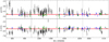 |
Fig. 1 R-band relative Stokes parameters of VI Cyg 12 (black circles) in comparison with two other standards: BD+32.3739 (blue triangles) and HD 212311 (green squares). The horizontal red lines and the pink areas represent Q/I and U/I values for VI Cyg 12 from Schmidt et al. (1992) with corresponding uncertainties. For ease of visualization, the values for the two other stars are shifted so that their average Stokes parameters match the red line. In spite of larger photon noise uncertainties, it is clear that the Stokes parameters of VI Cyg 12 are significantly variable and systematically deviate from their catalog values during long periods of time. |
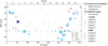 |
Fig. 2 Distribution of the sample stars over the sky. Samples B, H, L, and Z are described in Sect. 2. Fourteen stars marked as “not observed” and that have zero measurements were excluded from the final sample. Highly polarized and unpolarized stars are standards used in the previous studies listed in Table 1. The symbol size indicates polarization of individual stars from Table A.4. |
3 Observations and data reduction
We monitored the linear polarization parameters of the sample of candidate stars for four consecutive years in order to confirm their stability. The monitoring was performed using the RoboPol polarimeter. Additionally, we performed single-epoch measurements of a small subsample using the Nordic Optical Telescope. These observations are described in the following subsections.
3.1 RoboPol monitoring and data reduction
We carried out our polarimetric monitoring of the selected sample in the Cousins R-band and SDSS r′-band from May 2017 to June 2021 using the RoboPol polarimeter at the 1.3 m telescope of the Skinakas observatory. Every year observations are performed from May to November. Because the observatory does not operate during winter months, sources around RA = 12 h were insufficiently sampled. Of the initial 121 stars selected for monitoring, 14 were never observed or have poor quality of measurements. For this reason, they were dropped from the sample. However, most of them were located near other stars in the sample, and therefore would not increase much the sky coverage of our final standards catalog.
The polarizing assembly of the polarimeter consists of two half-wave plates and two Wollaston prisms aligned in such a way that any incident ray is split into four rays or channels with the polarization state rotated by 45° with respect to each other. RoboPol has no moving parts except the filter wheel, which simplifies operations and instrumental polarization modeling. Three Stokes parameters q = Q/I, u = U/I, and I (the last only when stars with known magnitude are present in the 13 × 13 arcmin FoV) can be measured simultaneously with a single exposure. The optical and mechanical design of RoboPol is described in Ramaprakash et al. (2019). All data for this program were collected in the central masked region of the FoV where systematic uncertainties are <0.1% (Ramaprakash et al. 2019).
The data were processed using the standard RoboPol pipeline, which is described by King et al. (2014), with modifications presented by Blinov et al. (2021). Further corrections were introduced at the calibration stage using known standard stars measurements. The details of this process are described below.
Standard processing of RoboPol data includes an instrumental polarization correction model. This model was created based on combined measurements obtained during multiple years of several unpolarized standard stars in a grid of hundreds of positions uniformly covering the FoV (King et al. 2014). Therefore, it approximates well the large-scale instrumental polarization variation across the entire FoV. However, we discovered that for stars measured in the central masked area there is a residual instrumental polarization that is unaccounted for by the model, and that depends on the (x, y) source position on the CCD. In Fig. 3 we show an example of such subtle instrumental polarization changes for unpolarized standards measured in 2019. A clear position-dependent trend with an amplitude of ~0.5% in the measured values of relative Stokes parameters can be seen. Since all measurements discussed in this work were observed in the central masked area, we had to correct them for this trend. We approximated these  and
and  dependences with a quadratic surface for each observing season separately. Using these fits, we corrected all measurements of corresponding seasons. Then, we determined the standard deviations in the q and u estimates for the unpolarized standards, and propagated these values with the corresponding uncertainties of standard candidates measurements.
We found the rotation of the instrumental q–u plane with respect to the standard reference frame using highly polarized standards (Table 1) that were monitored along with the standard candidates sample. Since individual catalog values for these standards are unreliable (see Sect. 1), we used a statistical approach: the entire sample was considered, including stars that are known to be variable (e.g., VI Cyg 12). For each standard we computed the weighted mean of the relative Stokes parameters combining all measurements along the observing period. Then, using these q, u estimates, we calculated the corresponding EVPArbpl values of each star in our measurements, and found the difference between this value and that reported in the literature, EVPAcat. For stars with multiple values reported in the literature, we used either the value with the smallest uncertainty, or the most recent measurement if the uncertainties are comparable. The EVPAcat values used are flagged with asterisks in Table 1. The corresponding differences between the RoboPol and literature estimates are shown in Fig. 4. We found the weighted mean of EVPArbpl – EVPAcat to be 1.1 ± 0.5°, after applying 3σ-clipping, which excluded CMaR1 24 from the averaging. This value was used as the instrumental EVPA zero-point correction, and all measurements were adjusted for it, while uncertainties were propagated accordingly.
We assessed the possibility that the polarimeter has a crosstalk between the relative Stokes parameters by measuring their covariance. We first corrected the measurements of unpolarized standards for the polarization and EVPA zero points as described before. Then, we calculated the correlation coefficient between q and u for each individual standard. There was no significant systematic correlation found among stars. We also calculated the correlation coefficient r for a set of standard star measurements for each season. In all cases |r| does not exceed 0.42, while the median value among seasons is r = −0.17. Therefore, we conclude that the crosstalk between channels of the polarimeter is negligible with respect to the noise level.
We also verified that the polarimetric efficiency of the instrument is 100% within measurement errors (i.e., the measured polarimetric accuracy is independent of the source polarization). To this end, we corrected the Stokes parameters of the highly polarized stars for the zero points, and then compared them with the corresponding literature values. The orthogonal distance regression fits to the data are consistent with the expected qrbpl = qcat and urbpl = ucat dependences within 1σ, as shown in Fig. 5.
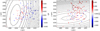 |
Fig. 3 Relative Stokes parameters of zero-polarization standards from Table 1 observed in 2019 in the central masked area as a function of the position on the CCD. The color of the points indicates the deviation of Q/I or U/I from zero (see color bars). The planar contours show the fitted quadratic surface. |
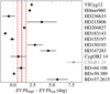 |
Fig. 4 Differences between weighted average of observed EVPA and corresponding catalog values for the 14 most reliable highly polarized standards. Weighted mean value for 13 stars (CMaR1 24 is excluded by 3σ-clipping) is shown by the solid red line, while the standard error of the mean is shown by the red dashed lines. |
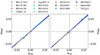 |
Fig. 5 Weighted mean values of Stokes parameters of high-polarization standards, as measured by RoboPol vs. catalog values from Table 1. The black dashed line is y = x; the red solid line is the ordinary least-squares regression fit to the data. The light blue region is the 1σ uncertainty region of the fit. |
3.2 NOT observations and data analysis
We selected a subset of ten standard candidates based on visibility, limited available observing time for this program, and preliminary stability observed in the RoboPol data. Subsequently, we conducted observations of these candidates using the Nordic Optical Telescope (NOT) under proposal 61-608. The Alhambra Faint Object Spectrograph and Camera (ALFOSC) instrument3 was used in its polarimetric mode. It is a two-channel polarimeter consisting of a rotating half-wave plate (HWP) and a calcite plate. For each object, two beam images called o and e are formed, corresponding to the 0° and 90° polarizations coming out of the WP, respectively. Standard candidates were observed with sequences consisting of eight exposures, corresponding to HWP positions of 0° to 180° in steps of 22.5°. This yields four Q/I and U/I measurements for each star. Observations were performed during the nights of 8 and 23 September and 13 December 2020 in multiple filters. Most of the stars were observed in SDSS ɡ-, r-, and i-bands and Johnson-Cousins B-, V-, and R-bands, while two stars were also observed in the U-band. Unpolarized standard stars BD+28.4211, HD 212311, and highly polarized standards Hiltner 960, VI Cyg 12, BD+59.389, BD+64.106, HD 204827 were observed during the same nights as the program targets. These standards were observed with sequences consisting of 16 exposures corresponding to HWP positions of 0° to 360° in steps of 22.5°. This provided eight Q/I and U/I measurements for each star.
For the analysis of the raw data, we developed a semi-automated data reduction pipeline in Python. Attention was paid to error estimation and propagation in each step of the analysis. Photometry was done using the aperture photometry package of the Photutils library4. To find the polarization parameters, we followed the procedure from Patat & Romaniello (2006). For each HWP position {θi = i × 22.5° | i ∈ {0, 1,…, N}} we calculated the normalized flux differences between the o and e star images:
 (1)
(1)
Then the relative Stokes parameters were expressed as
 (2)
(2)
 (3)
(3)
Using these q and u estimates, we inferred PD and EVPA, and their uncertainties as described in Sect. 3.3. Then we examined dependences of the PD and EVPA estimates on the photometry aperture radius, and selected optimal aperture and annulus radii, where both parameters reach a plateau and minimal uncertainties. The same procedure was performed for the observations of the standard stars. Using their polarization parameters, we found the instrumental polarization and EVPA zero points in each band individually. However, in the U-band, no standards were observed either during our observations or during adjacent nights. In the SDSS ɡ- and r-bands, only a single standard star measurement (BD+28.4211) was available. Therefore, we fitted the dependences of the instrumental q and u on the effective wavelength using all other bands with a linear function. By utilizing these fits, we determined the instrumental zero points of the relative Stokes parameters in each band and applied corrections to all measurements based on these values.
3.3 Polarization parameter estimates and their uncertainties
The polarization degree and its uncertainty were calculated assuming that the relative Stokes parameters q = Q/I and u = U/I follow a normal distribution:
 (4)
(4)
Any linear polarization measurement is biased towards higher PD values (Serkowski 1958). The PD follows a Rician distribution (Rice 1945) and significantly deviates from the normal distribution at low signal-to-noise ratios. There are a variety of methods suggested for correction of this bias (e.g., Simmons & Stewart 1985; Vaillancourt 2006). Our catalog provides the flexibility to select any debiasing method as the relative Stokes parameters constitute our ultimate data product. The data presented in this paper remain uncorrected for polarization bias. The relative Stokes parameters themselves are unbiased quantities.
The EVPA is defined as
 (5)
(5)
while its measurements are also non-Gaussian and defined by the following probability density (Naghizadeh-Khouei & Clarke 1993):
![Mathematical equation: $ G\left( {\theta ;{\theta _o};\,{\rm{P}}{{\rm{D}}_o}} \right) = {1 \over {\sqrt \pi }}\left\{ {{1 \over {\sqrt \pi }} + {\eta _o}{e^{\eta _o^2}}\left[ {1 + {\rm{erf}}\left( {{\eta _o}} \right)} \right]} \right\}\exp \left( { - {{{\rm{PD}}_o^2} \over {2\sigma _{{\rm{PD}}}^2}}} \right). $](/articles/aa/full_html/2023/09/aa46778-23/aa46778-23-eq13.png) (6)
(6)
Here  , erf is the Gaussian error function, PDo and θo are the true values of PD and EVPA, and σPD is the uncertainty of PD5.
We determine the EVPA uncertainty σθ numerically, by solving the following integral:
 (7)
(7)
The true value of PD in this procedure was estimated following Vaillancourt (2006) as
 (8)
(8)
For high S/N values, PD/σPD ≥ 20, the uncertainty of EVPA was approximated as σθ = PD/(2σPD).
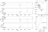 |
Fig. 6 Evolution of polarization parameters of B_0017+8135_82, which is found to be variable. (a, b) Evolution of the relative Stokes parameters. The dashed black line shows the weighted average; the red dashed lines show the corresponding 1 σ uncertainty. (c) Distribution of measurements on the relative Stokes parameters plane. (d, e) Evolution of the polarization degree and the electric vector position angle. The dashed black line shows the weighted average; the red dashed lines show the corresponding 1σ uncertainty. (f) EDF of measured polarization in both bands together with expected CDF of polarization measurements for a constant source with similar uncertainties. |
4 Analysis of variability
We assessed the variability of the sample stars following Clarke et al. (1993) and Bastien et al. (2007). The method can be summarized as follows. If the measurements of the relative Stokes parameters q and u are independent and follow normal distributions with means q0 and u0, then the statistic
 (9)
(9)
as demonstrated by Simmons & Stewart (1985), follows the Rician distribution (Rice 1945)
 (10)
(10)
where i is the unit imaginary number, J0 is the zeroth order Bessel function, and  . In the case of an unpolarized source (℘0 = 0), Eq. (10) reduces to the Rayleigh distribution:
 (11)
(11)
Then, the cumulative distribution function (CDF) of ℘ is expressed as:
 (12)
(12)
In practice, the CDF is approximated by the empirical cumulative distribution function (EDF):
 (13)
(13)
The EDF can deviate significantly from the CDF in two cases: (1) the source has variable polarization; (2) the uncertainties σq and σu are incorrectly estimated. Since in either of these cases the measurements of a star cannot be considered for establishing it as a standard, we do not distinguish between them.
In the case of a polarized source, its weighted means of the measured normalized Stokes parameters  and ū were used as estimates for q0 and u0 in order to reduce the polarization to zero:
 (14)
(14)
In order to assess whether the EDF significantly deviates from the CDF of a constant source given by Eq. (12), we used a two-sided Kolmogorov–Smirnov (KS) test. If the p-value of the KS test exceeds a given threshold, we consider the star to be non-variable and suitable for use as a standard. Otherwise, we consider it unsuitable. As mentioned earlier, if the p-value of the KS test is below the threshold, the star may indeed be variable or our uncertainty estimates of its measurements may be incorrect. We do not discriminate between these two cases. We use a threshold of p = 0.0455, corresponding to a 2σ confidence level, to assess the variability of stars. However, we also provide the p-values for all stars in the sample with ≥5 measurements in Table A.4. This enables the choice of a robust set of standards by filtering stars according to the p-value and opting for an alternate level of confidence. We do not perform the test for stars with fewer than five measurements, and mark them as uncertain.
We note that in the procedure described above the variability evaluation is based purely on the fractional polarization behavior, while information about the EVPA is completely ignored. However, there is a possibility that in peculiar cases the polarization vector can produce nearly perfect loops on the Q/I–U/I plane. In such a situation, the ℘reduced remains constant, while the EVPA changes with time. For instance, binary stars with envelopes symmetric about their orbital plane can produce such polarization variability (Brown et al. 1978). In order to avoid identification of stars with this variability pattern as stable, we visually inspected distributions of measurements on the relative Stokes parameters plane for each source. We did not find any false stable stars during this inspection.
Average polarization parameters of stable (2σ S.L.) stars in the established sample of standards.
5 Results
We obtained 696 R-band and 296 SDSS r′-band measurements of 107 stars with RoboPol, which are listed in Table A.2. Additionally, for nine stars we obtained multi-band polarization measurements with ALFOSC, which are presented in Table A.3. We did not find any significant systematic difference in relative Stokes parameters between the R- and r′-bands. Therefore, we combined all measurements in these two bands and considered them together. For each star in the sample, we constructed plots of the time series data showing the evolution of the fractional polarization PD, the EVPA, and the relative Stokes parameters Q/I and U/I. These monitoring data were analyzed using the method described in Sect. 4, so that the EDF of the normalized fractional polarization given by Eq. (14) was computed for each star. Then we compared it with the distribution given by Eq. (12), which is the expected cumulative distribution of the same quantity for a stable source with the same noise level. The time series, CDF, EDF, and the distribution of measurements on the relative Stokes parameters plane for B_0017+8135_82, as an example, are shown in Fig. 6. Similar plots for all other sources in the sample are only available online6. As the result, we found the average polarimetric parameters for each star in the sample and classified them as stable or variable with the 2σ confidence level. These parameters and classes are listed in Table A.4. For convenience, we list only the stable stars in a separate Table 2, together with their average relative Stokes parameters and Gaia’s G-band magnitude. We arbitrarily place the limit between highland low-polarization stars at PD = 0.5% in Table 2. This information, along with finding charts for all sample stars, can also be accessed online7.
6 Notes on individual stars
Several stars in the sample exhibited unexpected polarization or variability. We list these sources below with a brief description of their peculiar properties.
L_PG2349+002, L_92_249, L_92_248, L_111_1969, and L_PG2213–006A were selected among the Landolt photometric standards, that is, they were expected to have stable total flux density. However, these stars exhibit significant polarization variability.
H_GSC02355 was selected as a high-polarization star from Heiles (2000), where it has PD = 5.058%. However, in our measurements, this star is variable and has a higher average polarization of 6.0%. H_HD57702 was selected as a low-polarization star from Heiles (2000), where it has a PD of 0.040 ± 0.069%. However, in our measurements, this star is 0.33% polarized.
For stars L_PG1323–085D, Z_HD153752, H_HD344776, and L_111_1969, the EDF of the reduced PD (see Sect. 4) is located entirely to the left of the theoretical CDF. It means that these stars are more stable than one would expect from the uncertainties of their PD measurements. Since we used the two-sided KS test, these stars are classified as variable. However, it is likely that the uncertainties in the relative Stokes parameters for these four sources are overestimated, and the stars are in fact stable.
7 Conclusions
We obtained 1044 polarization measurements of 107 stars using two different polarimeters. Most observations were performed in the Cousins R-band and the SDSS r′-band with the RoboPol polarimeter along a 4-yr time interval. After applying a variability analysis to these monitoring data, we selected 65 stars that have five or more measurements and do not demonstrate significant variability in linear polarization in the red bands. These stars are listed in Table 2, and they can be used as optical polarimetric standards for calibration of instrumental polarization. For 24 stars, we did not have enough data to conclude whether they are variable or stable, while the remaining 18 stars were found to exhibit significant variability in polarization.
Acknowledgements
We thank T. Pursimo and S. Armas Pérez for assistance with the NOT observations. D.B., S.K, N.M., V.P., R.S., and K.T. acknowledge support from the European Research Council (ERC) under the European Union Horizon 2020 research and innovation program under the grant agreement no. 771282. A.S. acknowledges the Polish National Science Centre grant 2017/25/B/ST9/02805. This work was supported by the NSF grant AST-2109127. The data presented here were obtained in part with ALFOSC, which is provided by the Instituto de Astrofisica de Andalucia (IAA) under a joint agreement with the University of Copenhagen and NOT.
Appendix A Sample star information and monitoring data
Standard candidates sample information.
Polarimetric monitoring data.
Multiband single epoch measurements with ALFOSC/NOT.
Average polarization parameters of the sample stars.
References
- Bailey, J., & Hough, J. H. 1982, PASP, 94, 618 [NASA ADS] [CrossRef] [Google Scholar]
- Bastien, P., Drissen, L., Menard, F., et al. 1988, AJ, 95, 900 [NASA ADS] [CrossRef] [Google Scholar]
- Bastien, P., Vernet, E., Drissen, L., et al. 2007, ASP Conf.Ser., 364, 529 [NASA ADS] [Google Scholar]
- Berdyugin, A., & Teerikorpi, P. 2002, A&A, 384, 1050 [NASA ADS] [CrossRef] [EDP Sciences] [Google Scholar]
- Berdyugin, A., Piirola, V., & Teerikorpi, P. 2014, A&A, 561, A24 [NASA ADS] [CrossRef] [EDP Sciences] [Google Scholar]
- Blinov, D., Kiehlmann, S., Pavlidou, V., et al. 2021, MNRAS, 501, 3715 [NASA ADS] [CrossRef] [Google Scholar]
- Breus, V., Kolesnikov, S. V., & Andronov, I. L. 2021, A&A submitted, [arXiv:2112.12277] [Google Scholar]
- Brown, J. C., McLean, I. S., & Emslie, A. G. 1978, A&A, 68, 415 [NASA ADS] [Google Scholar]
- Carrasco, L., Strom, S. E., & Strom, K. M. 1973, ApJ, 182, 95 [NASA ADS] [CrossRef] [Google Scholar]
- Chentsov, E. L., Klochkova, V. G., Panchuk, V. E., Yushkin, M. V., & Nasonov, D. S. 2013, Astron. Rep., 57, 527 [NASA ADS] [CrossRef] [Google Scholar]
- Cikota, A., Patat, F., Cikota, S., & Faran, T. 2017, MNRAS, 464, 4146 [Google Scholar]
- Clarke, D. 2009, Stellar Polarimetry (Germany: Wiley-VCH) [CrossRef] [Google Scholar]
- Clarke, D., & Naghizadeh-Khouei, J. 1994, AJ, 108, 687 [NASA ADS] [CrossRef] [Google Scholar]
- Clarke, D., Naghizadeh-Khouei, J., Simmons, J. F. L., & Stewart, B. G. 1993, A&A, 269, 617 [NASA ADS] [Google Scholar]
- Clemens, D. P., & Tapia, S. 1990, PASP, 102, 179 [NASA ADS] [CrossRef] [Google Scholar]
- Dolan, J. F., & Tapia, S. 1986, PASP, 98, 792 [NASA ADS] [CrossRef] [Google Scholar]
- Gil-Hutton, R., & Benavidez, P. 2003, MNRAS, 345, 97 [NASA ADS] [CrossRef] [Google Scholar]
- Heiles, C. 2000, AJ, 119, 923 [Google Scholar]
- Hsu, J. C., & Breger, M. 1982, ApJ, 262, 732 [NASA ADS] [CrossRef] [Google Scholar]
- King, O. G., Blinov, D., Ramaprakash, A. N., et al. 2014, MNRAS, 442, 1706 [NASA ADS] [CrossRef] [Google Scholar]
- Landolt, A. U. 1992, AJ, 104, 340 [Google Scholar]
- Maharana, S., Anche, R. M., Ramaprakash, A. N., et al. 2022, J. Astron. Telescopes Instrum. Syst., 8, 038004 [NASA ADS] [Google Scholar]
- Naghizadeh-Khouei, J., & Clarke, D. 1993, A&A, 274, 968 [NASA ADS] [Google Scholar]
- Patat, F., & Romaniello, M. 2006, PASP, 118, 146 [Google Scholar]
- Piirola, V., Berdyugin, A., Frisch, P. C., et al. 2020, A&A, 635, A46 [NASA ADS] [CrossRef] [EDP Sciences] [Google Scholar]
- Ramaprakash, A. N., Rajarshi, C. V., Das, H. K., et al. 2019, MNRAS, 485, 2355 [NASA ADS] [CrossRef] [Google Scholar]
- Rice, S. O. 1945, Bell Syst. Tech. J., 24, 46 [Google Scholar]
- Schmidt, G. D., Elston, R., & Lupie, O. L. 1992, AJ, 104, 1563 [Google Scholar]
- Serkowski, K. 1958, Acta Astron., 8, 135 [NASA ADS] [Google Scholar]
- Simmons, J. F. L., & Stewart, B. G. 1985, A&A, 142, 100 [NASA ADS] [Google Scholar]
- Skalidis, R., Panopoulou, G. V., Tassis, K., et al. 2018, A&A, 616, A52 [NASA ADS] [CrossRef] [EDP Sciences] [Google Scholar]
- Tinbergen, J. 2007, PASP, 119, 1371 [NASA ADS] [CrossRef] [Google Scholar]
- Turnshek, D. A., Bohlin, R. C., Williamson, R. L., II et al. 1990, AJ, 99, 1243 [NASA ADS] [CrossRef] [Google Scholar]
- Vaillancourt, J. E. 2006, PASP, 118, 1340 [Google Scholar]
- Whittet, D. C. B., Martin, P. G., Hough, J. H., et al. 1992, ApJ, 386, 562 [NASA ADS] [CrossRef] [Google Scholar]
- Wiersema, K., Higgins, A. B., Covino, S., & Starling, R. L. C. 2018, PASA, 35, e012 [NASA ADS] [CrossRef] [Google Scholar]
- Wiktorowicz, S. J., Słowikowska, A., Nofi, L. A., et al. 2023, ApJS, 264, 42 [NASA ADS] [CrossRef] [Google Scholar]
- You, C., Zabludoff, A., Smith, P., et al. 2017, ApJ, 834, 182 [NASA ADS] [CrossRef] [Google Scholar]
- Zejmo, M., Słowikowska, A., Krzeszowski, K., Reig, P., & Blinov, D. 2017, MNRAS, 464, 1294 [NASA ADS] [CrossRef] [Google Scholar]
The equation for ηo is missing the factor of 2 for the cosine argument in Clarke (2009); the correct formula is provided in Naghizadeh-Khouei & Clarke (1993).
All Tables
Polarization parameters of standard stars monitored by RoboPol, as reported in the literature.
Average polarization parameters of stable (2σ S.L.) stars in the established sample of standards.
All Figures
|
Fig. 1 R-band relative Stokes parameters of VI Cyg 12 (black circles) in comparison with two other standards: BD+32.3739 (blue triangles) and HD 212311 (green squares). The horizontal red lines and the pink areas represent Q/I and U/I values for VI Cyg 12 from Schmidt et al. (1992) with corresponding uncertainties. For ease of visualization, the values for the two other stars are shifted so that their average Stokes parameters match the red line. In spite of larger photon noise uncertainties, it is clear that the Stokes parameters of VI Cyg 12 are significantly variable and systematically deviate from their catalog values during long periods of time. |
| In the text | |
|
Fig. 2 Distribution of the sample stars over the sky. Samples B, H, L, and Z are described in Sect. 2. Fourteen stars marked as “not observed” and that have zero measurements were excluded from the final sample. Highly polarized and unpolarized stars are standards used in the previous studies listed in Table 1. The symbol size indicates polarization of individual stars from Table A.4. |
| In the text | |
|
Fig. 3 Relative Stokes parameters of zero-polarization standards from Table 1 observed in 2019 in the central masked area as a function of the position on the CCD. The color of the points indicates the deviation of Q/I or U/I from zero (see color bars). The planar contours show the fitted quadratic surface. |
| In the text | |
|
Fig. 4 Differences between weighted average of observed EVPA and corresponding catalog values for the 14 most reliable highly polarized standards. Weighted mean value for 13 stars (CMaR1 24 is excluded by 3σ-clipping) is shown by the solid red line, while the standard error of the mean is shown by the red dashed lines. |
| In the text | |
|
Fig. 5 Weighted mean values of Stokes parameters of high-polarization standards, as measured by RoboPol vs. catalog values from Table 1. The black dashed line is y = x; the red solid line is the ordinary least-squares regression fit to the data. The light blue region is the 1σ uncertainty region of the fit. |
| In the text | |
|
Fig. 6 Evolution of polarization parameters of B_0017+8135_82, which is found to be variable. (a, b) Evolution of the relative Stokes parameters. The dashed black line shows the weighted average; the red dashed lines show the corresponding 1 σ uncertainty. (c) Distribution of measurements on the relative Stokes parameters plane. (d, e) Evolution of the polarization degree and the electric vector position angle. The dashed black line shows the weighted average; the red dashed lines show the corresponding 1σ uncertainty. (f) EDF of measured polarization in both bands together with expected CDF of polarization measurements for a constant source with similar uncertainties. |
| In the text | |
Current usage metrics show cumulative count of Article Views (full-text article views including HTML views, PDF and ePub downloads, according to the available data) and Abstracts Views on Vision4Press platform.
Data correspond to usage on the plateform after 2015. The current usage metrics is available 48-96 hours after online publication and is updated daily on week days.
Initial download of the metrics may take a while.