| Issue |
A&A
Volume 677, September 2023
|
|
|---|---|---|
| Article Number | A37 | |
| Number of page(s) | 12 | |
| Section | Numerical methods and codes | |
| DOI | https://doi.org/10.1051/0004-6361/202346547 | |
| Published online | 30 August 2023 | |
Estimating the selection function of Gaia DR3 subsamples
1
Leiden Observatory, Leiden University,
Niels Bohrweg 2,
2333 CA
Leiden, The Netherlands
e-mail: This email address is being protected from spambots. You need JavaScript enabled to view it.
2
Max-Planck-Institut für Astronomie,
Königstuhl 17,
69117
Heidelberg, Germany
3
INAF–Osservatorio Astrofisico di Torino,
Strada Osservatorio 20, Pino Torinese
10025
Torino, Italy
4
Institute of Astronomy, University of Cambridge,
Madingley Road,
Cambridge
CB3 0HA, UK
5
School of Physics and Astronomy, Monash University,
VIC
3800, Australia
6
Centre of Excellence for Astrophysics in Three Dimensions (ASTRO-3D),
Melbourne, Victoria, Australia
7
Center for Computational Astrophysics, Flatiron Institute,
162 Fifth Ave,
New York, NY
10010, USA
Received:
30
March
2023
Accepted:
17
June
2023
Abstract
Context. Understanding the intricacies behind the presence and absence of sources in an astronomical catalogue is crucial for the accurate interpretation of astronomical data. In particular, for the multi-dimensional Gaia data, filters and cuts on different parameters or measurements introduce a selection function that may unintentionally alter scientific conclusions in subtle ways.
Aims. We aim to develop a methodology to estimate the selection function for different subsamples of stars in the Gaia catalogue.
Methods. Comparing the number of stars in a given subsample to that in the overall Gaia catalogue provides an estimate of the subsample membership probability as a function of sky position, magnitude, and colour. The method used to make this estimate must differentiate the stochastic absence of subsample stars from selection effects. When multiplied with the overall Gaia catalogue selection function, this provides the total selection function of the subsample.
Results. We present our new method for estimating the selection function by applying it to the sources in Gaia DR3 with heliocentric radial velocity measurements. We also compute the selection function for the stars in the Gaia-Sausage/Enceladus sample, confirming that the apparent asymmetry of its debris across the sky is merely caused by selection effects.
Conclusions. The method we have developed estimates the selection function of the stars present in a subsample of Gaia data, given that the subsample is completely contained in the Gaia parent catalogue (for which the selection function is known). This tool is made available in a GaiaUnlimited Python package.
Key words: Galaxy: general / methods: statistical / catalogs
© The Authors 2023
 Open Access article, published by EDP Sciences, under the terms of the Creative Commons Attribution License (https://creativecommons.org/licenses/by/4.0), which permits unrestricted use, distribution, and reproduction in any medium, provided the original work is properly cited.
This article is published in open access under the Subscribe to Open model. This email address is being protected from spambots. You need JavaScript enabled to view it. to support open access publication.
1 Introduction
To reach meaningful scientific conclusions based on data for objects included in astronomical catalogues, we have to rely on the data and measurements these catalogues provide and, more importantly, we must know the caveats and limitations of the catalogue. The latter aspect includes understanding the kinds of objects are not included in the catalogue, which is often characterised by the catalogue selection function SC. Selection functions are commonly constructed through either understanding of the detection efficiency and chain of procedures used to build the catalogue, or through a statistical comparison of the catalogue with a ‘ground truth’, meaning a more complete set of sources of the same nature (for a review of the basics of astronomical selection functions, see Rix et al. 2021).
With the enormous wealth of data from recent astronomical missions, often scientific conclusions are reached based on specific subsamples generated by selecting certain kinds of objects (e.g. white dwarfs, red clump stars, or stars with available velocities) based on their attributes, rather than on the full catalogue. This is often the case when working with data from the Gaia mission (Gaia Collaboration 2016), which provides astrometric and photometric measurements for more than one billion stars in our Galaxy. In addition, it is common practice to apply additional quality cuts in order to remove undesired outliers. Every cut applied to produce a particular subsample (e.g. on colour, or using data quality flags) introduces different selection effects that must be accounted for. In the case of using Gaia data only, these selection effects can be taken into account by comparing the objects in any subsample against the full Gaia catalogue, the parent catalogue for which the completeness and selection function are assumed to be known.
Specific efforts to estimate the selection function for Gaia data were made following the appearance of the second Gaia data release (DR2, Gaia Collaboration 2018). Boubert et al. (2020, 2021) and Boubert & Everall (2020) used the epoch photometry of the variable stars in Gaia DR2 to estimate the Gaia parent catalogue selection function. Building on that work, Everall & Boubert (2022) computed the selection function for different subsamples of Gaia DR2 data, including the selection function of stars with heliocentric radial velocity (RV) measurements. This latter was also independently estimated by Rybizki et al. (2021), who took the ratio of sources with radial velocities compared to all Gaia DR2 sources. To estimate the parent catalogue selection function for Gaia DR3 (Gaia Collaboration 2023), Cantat-Gaudin et al. (2023) exploited the comparison of Gaia data with a deeper survey (the Dark Energy Camera Plane Survey, DECaPS, Schlafly et al. 2018; Saydjari et al. 2023) assumed to represent the ‘ground truth’ (i.e. to be 100% complete) in order to estimate the completeness of Gaia DR3 as a function of sky position and G magnitude. This latter work and the current paper are in the context of the GaiaUnlimited project1, the aim of which is to provide the community with selection functions for the different Gaia releases, as well as for different subsamples of the data, together with a Python package2 that contains the necessary tools for the application of different aspects of the Gaia selection function (scanning law, Gaia parent catalogue selection function, and several subsample selection functions and how to estimate them).
The goal of this paper is to provide the means to estimate the selection function of any subset of Gaia data. Figure 1 shows the cases where our methodology can be applied. The left and right panels show two examples of how to estimate the selection function when applying different filters (selection criteria) to the Gaia catalogue, where all the sources resulting from the filtering are included in the parent catalogue. In both cases, all the subsets shown can be drawn from simple queries to the Gaia archive. We stress again that we require the subsample to be entirely contained within the Gaia source catalogue, for which the selection function was empirically modelled by Cantat-Gaudin et al. (2023).
This paper is organised as follows. In Sect. 2, we describe the methodology used to estimate the selection function of a subset of Gaia data. We apply the method to the stars with heliocentric RV measurements in Gaia DR3 and compare our results with similar, previous methods in Sect. 3. Section 4 shows how to use the estimated selection function in a real science case, the Gaia-Sausage/Enceladus sample. Finally, we discuss our conclusions in Sect. 5. We also provide examples of the queries made in the Gaia archive in Appendix A, an example of the Python code to generate subsample selection functions using the GaiaUnlimited Python package in Appendix C and the selection function for different relevant subsets in Appendix D.
 |
Fig. 1 Sketch showing the cases where the proposed methodology can be applied. |
2 Method
Here we present a method to estimate the selection function of Gaia catalogue subsamples. These can be subsets drawn directly from the Gaia catalogue, or a set of sources included in another survey that was exclusively selected from the Gaia catalogue (e.g. a spectroscopic survey that draws its targets from Gaia). Our method relies on the fact that the Gaia catalogue is the parent catalogue to these subsamples, and that its basic selection function has already been well characterised. Generalising the cases sketched in Fig. 1, the probability Sc(q) that a source makes it into our subsample is described by (see Sect. 2.1 and Eq. (2) in Rix et al. 2021)
 (1)
(1)
where  describes the probability that a source with attributes q = {ℓ,b,G,…} will make it into the Gaia catalogue and Sc(q | q in parent) is the probability that a source will be in the subsample given that it is in the Gaia parent catalogue. The method we developed focuses on the estimation of Sc(q | q in parent), which then becomes a multiplicative factor to the parent catalogue selection function provided by Cantat-Gaudin et al. (2023) in estimating the total selection function of our subsample.
Probability of selecting the sources in the subsample
We model the number of sources that end up in our subsample as a binomial distribution, which assumes that sources are randomly selected with a given probability, which depends on the source attributes q. The binomial distribution is given by
 (2)
(2)
where n is the number of sources in the Gaia catalogue with attributes q, k is the number of sources with the same attributes that are contained in our subsample, and p is the probability that a source makes it into our subsample.
We estimate the value of p from the known values of n and k using a Bayesian approach. To estimate the posterior probability of p, we choose the beta distribution as a prior. This is a common choice because it is a conjugate prior probability distribution for the binomial distribution, meaning that the posterior probability of p is also a beta distribution, which is updated according to the data. We use an uninformative uniform prior distribution, which means a beta(α, β) distribution function with α = β = 1. In this particular case, and considering the above assumptions, the posterior distribution of p is given by beta (k + 1, n − k + 1), which has a mean value of
 (3)
(3)
and tends to k/n as k and n become larger. The variance of the beta (k + 1, n − k + 1) distribution function is given by
 (4)
(4)
Above, we summarise the full posterior distribution function in Eqs. (3) and (4). However, the advantage of using Bayesian statistics is that we have access to the full posterior distribution function for the probability p which, as already mentioned, is given by beta (k + 1, n – k + 1) in this case.
To apply the above method, the parent catalogue and sub-sample data are both binned by the attributes q, and n and k are recorded for each bin, from which p and its variance are then estimated according to the equations above. We then take SC(q | q in parent) = E(p). We note here that the parent catalogue selection function may explicitly depend on only a subset q′ of the attributes q used to select the subsample. It is assumed that  . This is illustrated in the following section.
In the limit of many stars, this estimate simply becomes the ratio of subsample-to-total Gaia stars. But if the number of subsample stars is small (or even zero), we must decipher whether this is because of selection effects or simply reflects the stochasticity of the sampling. Indeed, estimating the selection probability from the expected value given by Eq. (3) may produce biased results, particularly when both k and n are small. This is captured in the variance of the posterior distribution described in Eq. (4) (for low values of k and n, the variance will be higher and therefore the selection probability p is less constrained). To provide better insight into this, we evaluate in Fig. 2 the bias of our estimator for different ‘true’ probabilities p as a function of n. As expected, the bias of our estimate increases as n decreases and tends to zero for high values of n. Figure 2 can help us to fix a minimum value of stars in the Gaia catalogue per bin (n in our notation). For instance, for n ~ 20 stars, the maximum bias expected is around 5%. In the case of ptrue < 0.5, the expected E(p) can be severely overestimated for small n, and therefore bins containing larger values of n must be used. The suitable choice of bins to avoid these biases in the selection function estimate must be vetted for each application.
3 The selection function for stars with a heliocentric radial velocity in Gaia DR3
We now apply the method described in Sect. 2 to the sample of Gaia DR3 sources with available heliocentric RV measurements (Katz et al. 2023). To generate the data for estimating this selection function, we query the Gaia DR3 archive for the number of stars with heliocentric RV measurements as well as the number of stars in the Gaia DR3 parent catalogue (k and n in our notation, respectively). In Appendix A, we include an example of the query to retrieve the RV subsample in the desired format and an example of the resulting output is shown in Table A.1. We bin the data according to sky position (HEALPix), magnitude, and colour bins, and provide the selection function in every bin where both k and n are available. In the context of GaiaUnlimited, the RV selection function is provided in the Python package as DR3RVSSelectionFunction, corresponding to pre-computed sky maps at the resolution of HEALPix level 5, in 0.2 mag wide bins in G and 0.4 mag in G – GRP. As noted above, we assume here that  . Nevertheless, the selection function of the RV sample will be strongly dependent on colour. The explicit G – GRP dependence of the RV selection function is because the publication of RV measurements depends on the sources having an estimation of their GRVS magnitude and their effective temperature (Sartoretti et al. 2023). Both requirements can be well captured using the G – GRP colour as a proxy. Also, using G – GRP instead of GBP – GRP is preferred due to the known callibration issues of GBP at the faint end (Riello et al. 2021).
Figure 3 shows sky maps of the RV selection function at magnitude G = 13 and G – GRP = 0.5 in the top panel and G = 14 and G – GRP = 1 in the bottom panel, calculated according to Eq. (1). We note that, in this case, the term  describing the parent catalogue selection function is always 1 (in both cases) due to the bright G magnitude limit of the RV subsample3. We find low selection probability in the Galactic midplane, particularly in the Galactic centre where crowding effects are important. In the case of G = 14 and G – GRP = 1, the selection probability decreases as Galactic latitude increases; the selection function in these regions is underestimated due to noisy estimations of the selection function given the small values of both n and k for these extreme values of G and G – GRP (see Fig. 2 for an estimation of the bias as a function of n). We show the statistical uncertainty on both estimates in Fig. 4. The large number of sources near the Galactic plane makes the uncertainty (computed as the variance of the posterior probability distribution function in each HEALPix region) significantly smaller than at high Galactic latitudes, except for highly obscured regions.
To avoid bias and large uncertainties in an empirically evaluated completeness map, it is necessary to ensure that a sufficient number of sources are in the bins used to evaluate the selection function. In Fig. 3 we bin in magnitude, colour, and by HEALPix. One strategy to mitigate the problem of small number statistics is, for example, to adopt a sky map with variable resolution, adopting larger areas at high latitudes where there are fewer stars. Indeed, because of the bright magnitudes of the RV sample, the only dependence of the selection function on direction is due to crowding, and the selection function at high latitudes is only a function of G and G – GRP. In Fig. 5 we show the selection function for the RV sample as a function of G and G – GRP for b > 30 deg and b < 30 deg.
The selection function of the RV sample has dramatically improved in Gaia DR3 compared to EDR3 (where the RVs were inherited from Gaia DR2). The magnitude limit in this sample has increased from GRVS = 12 mag in Gaia EDR3 to GRVS = 14 mag in Gaia DR3, resulting in a total of approximately 33 million sources in the last data release compared to the approximately 7 million in EDR3. In Appendix B, we show a comparison of the improvement of the RV sample in Gaia DR3 with respect to Gaia EDR3, at G = 13 mag.
 |
Fig. 2 Bias of the probability estimator described by Eq. (3) for low values of n. The dash-dotted black line corresponds to an unbiased estimator, and the solid lines with different colours represent the experiment for different true probabilities ptrue ≥ 0.5. |
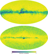 |
Fig. 3 Sky maps of the selection function for sources with available radial velocities at G = 13 and G – GRP = 0.5 (top panel), and G = 14 and colour G – Grp = 1 (bottom panel). These maps are shown at HEALPix level 5, with 0.2 mag bins in G and 0.4 mag bins in G – Grp. They manifestly depend on both magnitude and colour. |
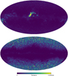 |
Fig. 4 Uncertainty in the selection function of stars with RV given by the variance of the posterior probability distribution function. The top panel corresponds to G = 13 and colour G – GRP = 0.5, and the bottom panel to G = 14 and colour G – GRP = 1. The sky maps correspond to the resolution of HEALPix level 5. |
 |
Fig. 5 Detection probability for the sources with available RV measurements at latitudes |b| > 30 deg, as a function of G magnitude and G – GRP colour. The width of the bins is 0.2 mag in G and 0.4 mag in G – GRP. |
Comparison to Everall & Boubert (2022)
Everall & Boubert (2022) estimated the selection function for three specific subsets of the Gaia EDR3 release. With precom-puted sky maps, the authors provide the probability that a source contained in Gaia EDR3 has (i) a reported parallax and proper motion, (ii) RUWE below 1.4, and (iii) a reported RV measurement as a function of sky position, G magnitude, and G – GRP colour (with this last dependence only for (ii) and (iii)). Briefly, their methodology describes the subset selection function as a sum of needlets across the sky where their coefficients are modelled by a Gaussian process prior in magnitude and colour (see Boubert & Everall 2022, for a detailed description). The use of needlets introduces spatial smoothing instead of estimating individual independent probabilities in each bin, which circumvents the problem of domination by noisy data. Similarly, the Gaussian processes introduce a correlation in the magnitude and colour dimensions.
As in our method described in Sect. 2, the core assumption of Everall & Boubert (2022) is that the probability to sample k stars out of n (from the parent catalogue) is described by the binomial likelihood distribution with a beta uniform distribution prior. Both approaches use the same data as the starting point (see Appendix A). Compared to our ratio-based method, the complex statistical model developed by Everall & Boubert (2022) comes with the advantage of providing an estimate of the selection function even when no data are available in a certain bin, and a more robust estimation for bins with a low number of stars. However, their forward-modelling approach is significantly more computationally expensive. While our running time is defined by the time of the query to the Gaia archive (typically of the order of tens of minutes), the statistical model in Everall & Boubert (2022) runs for approximately one week when parallelised over 88 cores, making the computation of custom subsample selection functions impractical.
In order to compare the method described by Everall & Boubert (2022) and the method we developed, we estimate the completeness of the sources with RVs in Gaia EDR3 using both methodologies (the actual condition is dr2_rv_nb_transits >= 4), which should provide similar results. Figure 6 shows sky maps of the selection function estimated with the Everall & Boubert (2022) method (left columns) and ours (right columns). We see a general agreement in the main features, namely the imprint of the scanning law for G = 12 mag and the initial Gaia source list (IGSL) at the faint end (G = 13 mag; shown in the top and bottom rows respectively), with our method being noisier due to the lack of smoothing between different bins. Given the similarities between the results of the two methodologies, we confirm that they provide similar results, with our method being a fast alternative to compute the selection function for any subsample of Gaia data. However, there is a notable offset which could be partly explained by the bias in our estimator (see Sect. 2).
4 Selection function for Gaia-Sausage/Enceladus
With the advent of Gaia DR2, and using the roughly 7 million sources with RVs, Helmi et al. (2018) reported a retrograde kinematic stellar structure in the nearby halo dubbed Gaia-Sausage/Enceladus (GS/E), which traces a major accretion event experienced by the Milky Way that contributed to the formation of its thick disc (see Belokurov et al. 2018, for details on its discovery in Gaia DR1). Helmi et al. (2018) selected stars belonging to GS/E as a set of cuts in the Gaia DR2 catalogue with available RVs to show the structure of its debris. These cuts include ϖ > 0.1 mas, ϖ/σϖ > 5, and −1500 < Lz < 150 kpc km s−1. The authors found that the GS/E debris covers the whole sky, with an asymmetric shape for the more distant stars (0.1 < ϖ < 0.25 mas, see their Fig. 3). Each of these cuts introduces a selection effect that can be accounted for when computing the selection function. As pointed out by Helmi et al. (2018), we find that the main source of the observed asymmetry in the GS/E debris is the selection effect caused by both the cuts in m and ϖ/σϖ. We used the method described in Sect. 2 to estimate the selection function of the stars in both Gaia DR2 and DR3 that satisfy the two parallax cuts. The result is shown in Fig. 7 as a function of sky position (the magnitude and colour dependencies have been marginalised out). The asymmetry (from top-left to bottom-right) is visible for both the Gaia DR2 and DR3 sub-samples, but is much less prominent in DR3. The imprint of the scanning law is less pronounced for DR3 as well, as expected due to its longer observational baseline and more homogeneous coverage of the celestial sphere.
In order to examine whether or not the selection effects from the cuts in ϖ and ϖ/σϖ can account for the asymmetry seen in the GS/E sample, we simulated a spherical distribution of red giant branch stars (RGBs) in the halo. We use a spherical, power-law density distribution to generate the mock RGB sample with a number density that follows n(r) ∝ r−2. While the true stellar density in the inner Galactic halo has a slightly steeper density profile (between 2 and 3; see, e.g., Deason et al. 2011), this qualitative demonstration of selection effects does not show a significant dependency on the density profile slope. We first generate 107 star particles following our adopted density profile within the range of 0 < r < 250 kpc with randomly chosen spherical angles φ, θ. To assign simulated photometry to the star particles, we use a single MIST isochrone (Dotter 2016; Choi et al. 2016) with an age τ = 10 Gyr and metallicity [Fe/H] = −1.5. We generate photometry for the star particles by uniformly sampling equivalent evolutionary points (EEPs) within the range of EEPs on the giant branch and use cubic spline interpolation to map the generated EEPs to photometric measurements computed along the isochrone. The star counts for the simulated distribution, summed over all magnitude bins, are shown in the top panel of Fig. 8 for HEALPix level 5. We then apply the selection function represented in Fig. 7 (corresponding to Gaia DR2) at different magnitude bins. For this, we simply multiply the number of stars in the simulation in each of the HEALPix and magnitude bins by the fraction of stars that would be selected after the application of the different cuts to estimate the expected number of stars in that bin. This is shown in the bottom panel of Fig. 8, where we can see that the application of the selection effects in ϖ and ϖ/σϖ results in an asymmetric distribution of the initially spherical distribution of RGB stars, confirming that this asymmetry is merely a selection effect.
In addition to the two parallax cuts whose selection function is displayed in Fig. 7, Helmi et al. (2018) performed an angular momentum cut retaining only stars with −1500 < Lz < 150 kpc km s−1. Figure 9 shows the selection functions for the cuts to produce the GS/E sample relative to Gaia DR2 and DR3, in the top and bottom panels, respectively. Much of the asymmetry seen in the Gaia DR2 sample is removed in DR3, which is due to a combination of the improved parallax precision and the larger volume explored by the stars with RVs. On the other hand, Fig. 9 reveals a stronger selection effect in Gaia DR3, favouring stars in the Galactic halo. The query to generate the relevant data to compute such a selection function differs from the query in Sect. 3 by its inclusion of the computation Lz, which is done outside the Gaia archive. The selection function is estimated from a sample of GS/E stars uploaded to the Gaia archive as a user table, which is cross matched to the Gaia source table by source_id. The query is provided in Appendix A.
 |
Fig. 6 Comparison of the method by Everall & Boubert (2022, left column) and the one developed in this paper (right column). The top panels show the Gaia EDR3 selection function for stars with RVs at G = 12 mag, while the bottom panels show the same selection function at G = 13 mag. The results from the two methodologies show good general agreement, capturing similar features in the sky maps, with the method developed by Everall & Boubert (2022) being a smooth version of the maps due to the inclusion of smoothing and correlation coefficients between different bins. All the maps correspond to a resolution of HEALPix level 5. |
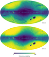 |
Fig. 7 Selection function for sources with ϖ > 0.1 mas and ϖ/σϖ> 5 mas. The top panel shows the case for Gaia DR2, while the bottom panel shows Gaia DR3. Both maps correspond to the resolution of HEALPix level 7. The magnitude and colour dependencies have been marginalised out. |
5 Summary
We developed a method to estimate the selection function, and its uncertainty, for subsets of the Gaia data. Our methodology provides the means to compute the probability that a source with certain attributes is included in a subsample provided the subsample is completely contained within the Gaia catalogue. To obtain the total selection function, this probability should be multiplied by the Gaia parent catalogue selection function (Cantat-Gaudin et al. 2023). Our method is computationally inexpensive (compared to previous methodologies for the same purpose; Everall & Boubert 2022), and allows the fast computation of subsample selection functions from the application of cuts on the Gaia archive or usergenerated data tables (see Appendix A). The whole method, together with full documentation, is provided in the Python package of the GaiaUnlimited project as a customisable class, SubsampleSelectionFunction (see Appendix C for a usage example).
We applied the described methodology to estimate the selection function of the subset of Gaia DR3 with heliocentric RV measurements, which are also provided as built-in functions in the GaiaUnlimited package. We find that the selection function for the stars with RVs is well constrained for well-populated bins in either the targeted subsample or the full catalogue (high k and n in our notation), and is less reliable when these numbers are low (as captured by the uncertainty in the selection function; see Fig. 4). For low values of k and n, we also characterised the bias of our estimation of the selection probability in Fig. 2, which can also help in selecting the binning of the data in order to have a minimum n in each bin. The main dependencies of the RV selection function are l, b, and G (following the main dependencies of the Gaia catalogue selection function) plus the additional dependence of G – GRP4. The addition of the colour as an argument of the selection function is to capture the temperature and the GRVS dependencies of the RV sample. We assume that the Gaia catalogue selection function depends on sky position (l, b) and G magnitude. A discussion on the inclusion of a colour dependency in the Gaia catalogue selection function is out of the scope of this paper. However, Cantat-Gaudin et al. (2023) found no evidence of such a dependency (see their Sect. 4 for a detailed discussion).
Section 4 represents an example of how the application of the selection function for subsamples of Gaia data can affect scientific conclusions. Other authors have used our GaiaUnlimited package to estimate the selection function for different subsamples tailored to their studies. Della Croce et al. (2023) estimated the selection function of the stars with a five-parameter solution (using Eq. (3)) in their study of ongoing hierarchical cluster assembly in the Perseus complex. Evans et al. (2023) used our selection function tools to show that the lack of firm hypervelocity star candidates in the Gaia DR3 RV sample provides constraints on a possible black hole companion to Sgr A* in the Galactic centre. In their discovery of the remnants of the proto-Milky Way residing in the central regions of our Galaxy, Rix et al. (2022) did not account for the selection function. Given that their study is based on a subset of Gaia DR3, the conclusions could be further refined by accounting for the selection function using the tools we present here. In general, all studies relying on the properties of samples selected from the Gaia catalogue could obtain more robust scientific conclusions by incorporating the methodology presented here.
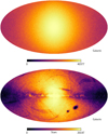 |
Fig. 8 Simulated sample of RGB stars before (top panel) and after (bottom panel) the application of the selection function accounting for the ϖ and π/σϖ selection effects. The asymmetry on the sample after the application of the selection function can be seen from the top-left to the bottom-right of the plot. The maps are computed at HEALPix level 5. |
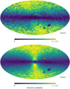 |
Fig. 9 Selection function for the sources selected to be part of GS/E, described by the sources with RVs, ϖ > 0.1 mas, ϖ/σϖ > 5 mas, and −1500 < Lz < 150 kpc km s−1, with respect to Gaia DR2 and DR3 in the top and bottom panels, respectively. The top panel belongs to the original sample in Gaia DR2 described by Helmi et al. (2018), while the bottom panel shows the same cuts applied to Gaia DR3. The maps correspond to the resolution of HEALPix level 4. The magnitude and colour dependencies have been marginalised out. |
Acknowledgements
We thank David W. Hogg for his contributions to the GaiaUnlimited project. This work is a result of the GaiaUnlimited project, which has received funding from the European Union’s Horizon 2020 research and innovation program under grant agreement No. 101004110. The GaiaUnlim-ited project was started at the 2019 Santa Barbara Gaia Sprint, hosted by the Kavli Institute for Theoretical Physics at the University of California, Santa Barbara. This work has made use of results from the European Space Agency (ESA) space mission Gaia, the data from which were processed by the Gaia Data Processing and Analysis Consortium (DPAC). Funding for the DPAC has been provided by national institutions, in particular, the institutions participating in the Gaia Multilateral Agreement. The Gaia mission website is http://www.cosmos.esa.int/gaia. The authors are current or past members of the ESA Gaia mission team and of the Gaia DPAC.
Appendix A Example query to the Gaia archive
The query below is an example of how to retrieve a table from the Gaia archive, with the needed information binned in sky position (HEALPix level 5, from source_id), magnitude G, and colour G – GRP. In this particular case, we show how to query the stars with available radial_velocity measurements. The G magnitude is binned from 3 to 20 in bins of 0.2 mag. For the G – GRP colour, the bin size is 0.4 mag in the range of −2.5 to 5.1.
The result of the query is shown in Table A.1, where, for a particular HEALPix pixel and G and G – GRP bin numbers, the total number of stars (n) and the number of stars fulfilling the specific selection (k) is retrieved.
SELECT magnitude, colour, position, COUNT(*) AS n, SUM(selection) AS k
FROM (SELECT to_integer(floor((phot_g_mean_mag - 3)/0.2)) AS magnitude,
	     to_integer(floor((g_rp + 2.5)/0.4)) AS colour,
	     to_integer(GAIA_HEALPIX_INDEX(5, source_id)) AS position,
	     to_integer(IF_THEN_ELSE(‘radial_velocity is not null’, 1.0, 0.0)) AS selection
	FROM gaiadr3.gaia_source
	WHERE phot_g_mean_mag > 3 AND phot_g_mean_mag < 20
	AND g_rp > -2.5 AND g_rp < 5.1) AS subquery
GROUP BY magnitude, colour, position
Values for the total number of stars in Gaia (n) and the number of stars with heliocentric RV measurements (k) binned in sky position (HEALPix index at level 5), magnitude G, and colour G – GRP.
Alternatively, if the selection function to be computed is that from a user-made table, given that all the sources are in the Gaia catalogue, the query to be performed in the Gaia archive relies on a cross match on source_id. The following query provides an example based on Sect. 4, where the Lz has been computed outside the Gaia archive and the resulting sample has been uploaded as user_acastr01.ges_dr3.
SELECT magnitude, colour, position, COUNT(*) AS n, SUM(selection) AS k
FROM (SELECT to_integer(floor((phot_g_mean_mag - 3)/0.2)) AS magnitude,
	     to_integer(floor((g_rp + 2.5)/0.4)) AS colour,
	     to_integer(GAIA_HEALPIX_INDEX(4, source_id)) AS position,
	     to_integer(IF_THEN_ELSE(
			‘source_id in (select source_id from user_acastr01.ges_dr3)’, 1.0,0.0)
	) AS selection
	FROM gaiadr2.gaia_source
	WHERE phot_g_mean_mag > 3 AND phot_g_mean_mag < 20
	AND g_rp > -2.5 AND g_rp < 5.1) AS subquery
GROUP BY magnitude, colour, position
Appendix B Comparison of the Gaia EDR3 and DR3 RV selection function
In this section, we compare the completeness of the RV sample in Gaia EDR3 with respectto Gaia DR3 atmagnitude G = 13, which is beyond the Gaia EDR3 magnitude limit. The coverage of the RV sample in Gaia DR3 has greatly improved, and the features such as the IGSL seen in Gaia EDR3 are removed.
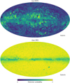 |
Fig. B.1 Completeness sky map at HEALPix level 5 of the sources with available RVs at magnitude G = 13 in Gaia EDR3 (top panel) and in Gaia DR3 (bottom panel). The dependency on colour has been marginalised out. |
Appendix C Using the GaiaUnlimited package
As part of the GaiaUnlimited Python package, we provide the class SubsampleSelectionFunction to generate selection functions for subsamples from the Gaia catalogue. The user is expected to provide the Gaia archive query that produces the subsample. Then, the selection function for the subsample is calculated according to the methodology outlined in Sect. 2.
The SubsampleSelectionFunction class takes three arguments: subsample_query, which is the query to be performed in the Gaia archive; file_name, which is used to store the data resulting from the query and save time in following executions of the same run; and a Python dictionary including the dimensions in which to bin the data and their binning. This dictionary should include the desired HEALPix level, and additional Gaia columns to bin the data. For instance, to generate a selection function at the resolution of HEALPix level 5, G ∈ [3,20] in steps of 0.2 and G – GRP – [−2.5, 5.1] in bins of 0.4, the expected dictionary is:
inDict = {‘healpix’: 5, ‘phot_g_mean_mag’: [3,20,0.2], ‘g_rp’: [-2.5,5.1,0.4]}.
Additional columns may be added as additional dependencies in the selection function, bearing in mind that this may increase the execution time (of the query) and decrease the number of stars (in both k and n in ournotation) in each bin, therefore increasing the noise and the number of regions of the sky with no available data (see Sect. 3).
Once the SubsampleSelectionFunction class has been initialised, the resulting selection function can be queried by providing the targeted coordinates (can be an array with the centres of the HEALPix pixels for an all-sky plot), magnitude G, colour G – GRP and the possible additional columns. To access the desired magnitude and colour bins (and any other dimension from Gaia columns), the name of the column plus an underscore (_) should be provided as the argument name (an example is shown in Listing 1).
Listing 1 shows the Python code used to generate one of the completeness maps shown in Fig. 3. The time to execute Listing 1 is dominated by the query to the archive (line 14) and in this case, is about 40 min.
We show further applications of the SubsampleSelectionFunction class by estimating the selection function for sources with (i) a measured parallax and proper motion and (ii) RUWE< 1.4. The completeness maps and the relevant change on the main code shown in Listing 1 are shown in the Appendix D.
Appendix D Example of other selection functions
Similarly to Everall & Boubert (2022), in this Appendix we show the completeness maps for the sources with (i) parallax and proper motion measurements (Fig. D.1), and (ii) RUWE < 1.4 (Fig. D.2). These selection functions are as a function of sky position only; the dependencies with magnitude and colour have been marginalised out. The code to generate these selection functions and completeness maps is similar to that in Listing 1, where the SubsampleSelectionFunction class has been initialised as shown in Listing 2.
 |
Fig. D.1 Completeness map at HEALPix level 5 of the sources with reported parallax and proper motions. The magnitude and colour dependencies have been marginalised out. |
 |
Fig. D.2 Completeness map at HEALPix level 5 for the sources with RUWE < 1.4. The magnitude and colour dependencies have been marginalised out. |
References
- Belokurov, V., Erkal, D., Evans, N. W., Koposov, S. E., & Deason, A. J. 2018, MNRAS, 478, 611 [Google Scholar]
- Boubert, D., & Everall, A. 2020, MNRAS, 497, 4246 [NASA ADS] [CrossRef] [Google Scholar]
- Boubert, D., & Everall, A. 2022, MNRAS, 510, 4626 [NASA ADS] [CrossRef] [Google Scholar]
- Boubert, D., Everall, A., & Holl, B. 2020, MNRAS, 497, 1826 [NASA ADS] [CrossRef] [Google Scholar]
- Boubert, D., Everall, A., Fraser, J., Gration, A., & Holl, B. 2021, MNRAS, 501, 2954 [NASA ADS] [CrossRef] [Google Scholar]
- Cantat-Gaudin, T., Fouesneau, M., Rix, H.-W., et al. 2023, A&A, 669, A55 [NASA ADS] [CrossRef] [EDP Sciences] [Google Scholar]
- Choi, J., Dotter, A., Conroy, C., et al. 2016, ApJ, 823, 102 [Google Scholar]
- Deason, A. J., Belokurov, V., & Evans, N. W. 2011, MNRAS, 416, 2903 [NASA ADS] [CrossRef] [Google Scholar]
- Della Croce, A., Dalessandro, E., Livernois, A., et al. 2023, A&A, 674, A93 [NASA ADS] [CrossRef] [EDP Sciences] [Google Scholar]
- Dotter, A. 2016, ApJS, 222, 8 [Google Scholar]
- Evans, F. A., Rasskazov, A., Remmelzwaal, A., et al. 2023, MNRAS, 525, 561 [NASA ADS] [CrossRef] [Google Scholar]
- Everall, A., & Boubert, D. 2022, MNRAS, 509, 6205 [Google Scholar]
- Gaia Collaboration (Prusti, T., et al.) 2016, A&A, 595, A1 [NASA ADS] [CrossRef] [EDP Sciences] [Google Scholar]
- Gaia Collaboration (Brown, A. G. A., et al.) 2018, A&A, 616, A1 [NASA ADS] [CrossRef] [EDP Sciences] [Google Scholar]
- Gaia Collaboration (Vallenari, A., et al.) 2023, A&A, 674, A1 [NASA ADS] [CrossRef] [EDP Sciences] [Google Scholar]
- Helmi, A., Babusiaux, C., Koppelman, H. H., et al. 2018, Nature, 563, 85 [Google Scholar]
- Katz, D., Sartoretti, P., Guerrier, A., et al. 2023, A&A, 674, A5 [NASA ADS] [CrossRef] [EDP Sciences] [Google Scholar]
- Riello, M., De Angeli, F., Evans, D. W., et al. 2021, A&A, 649, A3 [NASA ADS] [CrossRef] [EDP Sciences] [Google Scholar]
- Rix, H.-W., Hogg, D. W., Boubert, D., et al. 2021, AJ, 162, 142 [NASA ADS] [CrossRef] [Google Scholar]
- Rix, H.-W., Chandra, V., Andrae, R., et al. 2022, ApJ, 941, 45 [NASA ADS] [CrossRef] [Google Scholar]
- Rybizki, J., Rix, H.-W., Demleitner, M., Bailer-Jones, C. A. L., & Cooper, W. J. 2021, MNRAS, 500, 397 [Google Scholar]
- Sartoretti, P., Marchal, O., Babusiaux, C., et al. 2023, A&A, 674, A6 [NASA ADS] [CrossRef] [EDP Sciences] [Google Scholar]
- Saydjari, A. K., Schlafly, E. F., Lang, D., et al. 2023, ApJS, 264, 28 [NASA ADS] [CrossRef] [Google Scholar]
- Schlafly, E. F., Green, G. M., Lang, D., et al. 2018, ApJS, 234, 39 [Google Scholar]
https://github.com/gaia-unlimited/gaiaunlimited. The full documentation can be found in https://gaiaunlimited.readthedocs.io/en/latest/index.html
In other words, the parent Gaia DR3 catalogue is complete in the regions of the parameter space where Gaia RVs are available.
However, we note that when using the GaiaUnlimited package the user is free to select their own dependencies for the SubsampleSelectionFunction class in the form of an input dictionary.
All Tables
Values for the total number of stars in Gaia (n) and the number of stars with heliocentric RV measurements (k) binned in sky position (HEALPix index at level 5), magnitude G, and colour G – GRP.
All Figures
 |
Fig. 1 Sketch showing the cases where the proposed methodology can be applied. |
| In the text | |
 |
Fig. 2 Bias of the probability estimator described by Eq. (3) for low values of n. The dash-dotted black line corresponds to an unbiased estimator, and the solid lines with different colours represent the experiment for different true probabilities ptrue ≥ 0.5. |
| In the text | |
 |
Fig. 3 Sky maps of the selection function for sources with available radial velocities at G = 13 and G – GRP = 0.5 (top panel), and G = 14 and colour G – Grp = 1 (bottom panel). These maps are shown at HEALPix level 5, with 0.2 mag bins in G and 0.4 mag bins in G – Grp. They manifestly depend on both magnitude and colour. |
| In the text | |
 |
Fig. 4 Uncertainty in the selection function of stars with RV given by the variance of the posterior probability distribution function. The top panel corresponds to G = 13 and colour G – GRP = 0.5, and the bottom panel to G = 14 and colour G – GRP = 1. The sky maps correspond to the resolution of HEALPix level 5. |
| In the text | |
 |
Fig. 5 Detection probability for the sources with available RV measurements at latitudes |b| > 30 deg, as a function of G magnitude and G – GRP colour. The width of the bins is 0.2 mag in G and 0.4 mag in G – GRP. |
| In the text | |
 |
Fig. 6 Comparison of the method by Everall & Boubert (2022, left column) and the one developed in this paper (right column). The top panels show the Gaia EDR3 selection function for stars with RVs at G = 12 mag, while the bottom panels show the same selection function at G = 13 mag. The results from the two methodologies show good general agreement, capturing similar features in the sky maps, with the method developed by Everall & Boubert (2022) being a smooth version of the maps due to the inclusion of smoothing and correlation coefficients between different bins. All the maps correspond to a resolution of HEALPix level 5. |
| In the text | |
 |
Fig. 7 Selection function for sources with ϖ > 0.1 mas and ϖ/σϖ> 5 mas. The top panel shows the case for Gaia DR2, while the bottom panel shows Gaia DR3. Both maps correspond to the resolution of HEALPix level 7. The magnitude and colour dependencies have been marginalised out. |
| In the text | |
 |
Fig. 8 Simulated sample of RGB stars before (top panel) and after (bottom panel) the application of the selection function accounting for the ϖ and π/σϖ selection effects. The asymmetry on the sample after the application of the selection function can be seen from the top-left to the bottom-right of the plot. The maps are computed at HEALPix level 5. |
| In the text | |
 |
Fig. 9 Selection function for the sources selected to be part of GS/E, described by the sources with RVs, ϖ > 0.1 mas, ϖ/σϖ > 5 mas, and −1500 < Lz < 150 kpc km s−1, with respect to Gaia DR2 and DR3 in the top and bottom panels, respectively. The top panel belongs to the original sample in Gaia DR2 described by Helmi et al. (2018), while the bottom panel shows the same cuts applied to Gaia DR3. The maps correspond to the resolution of HEALPix level 4. The magnitude and colour dependencies have been marginalised out. |
| In the text | |
 |
Fig. B.1 Completeness sky map at HEALPix level 5 of the sources with available RVs at magnitude G = 13 in Gaia EDR3 (top panel) and in Gaia DR3 (bottom panel). The dependency on colour has been marginalised out. |
| In the text | |
 |
Fig. D.1 Completeness map at HEALPix level 5 of the sources with reported parallax and proper motions. The magnitude and colour dependencies have been marginalised out. |
| In the text | |
 |
Fig. D.2 Completeness map at HEALPix level 5 for the sources with RUWE < 1.4. The magnitude and colour dependencies have been marginalised out. |
| In the text | |
Current usage metrics show cumulative count of Article Views (full-text article views including HTML views, PDF and ePub downloads, according to the available data) and Abstracts Views on Vision4Press platform.
Data correspond to usage on the plateform after 2015. The current usage metrics is available 48-96 hours after online publication and is updated daily on week days.
Initial download of the metrics may take a while.


