| Issue |
A&A
Volume 677, September 2023
|
|
|---|---|---|
| Article Number | A109 | |
| Number of page(s) | 11 | |
| Section | Planets and planetary systems | |
| DOI | https://doi.org/10.1051/0004-6361/202245225 | |
| Published online | 12 September 2023 | |
Induction heating of planetary interiors in white dwarf systems
1
University of Vienna, Department of Astrophysics,
Türkenschanzstrasse 17,
1180
Vienna,
Austria
e-mail: This email address is being protected from spambots. You need JavaScript enabled to view it.
2
Freie Universität Berlin, Institute of Geological Sciences,
Malteserstrasse 74-100,
12249
Berlin,
Germany
3
Space Research Institute, Austrian Academy of Sciences,
Schmiedlstrasse 6,
8042
Graz,
Austria
4
Special Astrophysical Observatory of Russian Academy of Sciences,
Nizhny Arkhyz,
Zelenchukskaya
369167,
Russia
5
Bayerisches Geoinstitut, University of Bayreuth,
Universitätsstrasse 30,
95440
Bayreuth,
Germany
Received:
16
October
2022
Accepted:
9
June
2023
Abstract
Context. White dwarfs are the last evolutionary stage for the majority of main-sequence stars. With nuclear burning having ceased, these stars are slowly cooling. There is observational evidence indicating that planetary remnants, and possibly even planets, orbit a considerable fraction of the known white dwarf population. These objects are interesting targets for transit observations due to their large planet-to-star radius ratio. Especially interesting is the possible outgassing from such objects and their eventual observational prospects.
Aims. Here, we investigate whether electromagnetic induction heating can drive additional volcanic outgassing from small planetary remnants orbiting white dwarfs. This mechanism can be important for such bodies in addition to tidal heating due to the extremely strong magnetic fields of some white dwarfs and close orbital distances of planets to their host stars.
Methods. We calculated the heating and related magmatic effects for a Moon-sized body around a magnetized white dwarf using an analytical model for induction heating and a numerical model for interior processes. We also calculated induction heating inside asteroid-sized bodies.
Results. We show that induction heating can melt the mantle of a Moon-sized object within a geologically short time and contribute to desiccation of small asteroids on extremely tight orbits. These findings can have important implications for the evolution of rocky bodies orbiting white dwarfs and the potential detection of their outgassing.
Key words: planets and satellites: interiors / planet-star interactions / white dwarfs / methods: numerical / magnetic fields
© The Authors 2023
 Open Access article, published by EDP Sciences, under the terms of the Creative Commons Attribution License (https://creativecommons.org/licenses/by/4.0), which permits unrestricted use, distribution, and reproduction in any medium, provided the original work is properly cited.
This article is published in open access under the Subscribe to Open model. This email address is being protected from spambots. You need JavaScript enabled to view it. to support open access publication.
1 Introduction
White dwarfs (WDs) are post-main-sequence stars for which the nuclear fuel ceased to burn. They are very compact objects that do not possess any internal energy sources and slowly cool on a gigayear scale. Several works have suggested and attempted to detect planets orbiting WDs (e.g. Agol 2011; Faedi et al. 2011; Fossati et al. 2012; Sandhaus et al. 2016), and planetesimals within a debris disc, or even planetary candidates of a various nature, have been detected (e.g. Vanderburg et al. 2015, 2020; Manser et al. 2019; Gänsicke et al. 2019). Therefore, it is possible that some WDs host (as of yet undetected) planets and that many hosted planets in the past.
The indirect evidence that many WDs hosted or possibly still host a planetary system is the observation of metal pollution of WDs’ atmospheres atmospheres, indicating the presence of a debris disc around these stars with debris continuously falling onto the stellar surface (e.g. Vanderburg et al. 2015; Jura & Xu 2010, 2012). Recently, the accretion rate of planetary material was also determined from X-ray observations (Farihi et al. 2018; Cunningham et al. 2022). The survival of a main-sequence (MS) planetary system or formation of new planets around WDs has been considered by a variety of authors (e.g. Veras 2016, and references therein). Planets that survived the asymptotic giant branch (AGB) phase of their host stars’ evolution might migrate towards the star as a result of dynamical interactions or magnetic drag (Li et al. 1998). Furthermore, the Kozai-Lidov mechanism can bring planets close to WDs, assuming that the WDs have distant stellar companions (Stephan et al. 2021). Malamud & Perets (2016, 2017) show that even minor planets would be capable of keeping a significant amount of their water inventory throughout the most luminous phase of their host star’s evolution.
One of the differences between MS stars and WDs is the strengths of their magnetic fields. The strong global magnetic fields often observed in WDs (e.g. Bagnulo & Landstreet 2021) provide a much stronger environmental magnetic field around bodies orbiting such stars. Here, we consider the influence of such fields on the planets orbiting them. We investigate how the magnetic field of a strongly magnetized WD can influence a Moon-sized object orbiting it, which seems to be a good approximation for the size of some of the larger objects in debris disc around WDs. We also discuss the influence that induction heating could have on smaller asteroids with sizes of tens of kilometres. Our results are also applicable to closer planets orbiting WDs with weaker magnetic fields.
We consider a strongly magnetized WD with an average magnetic field of 13 million Gauss (MG)1 and a rotation period of 2 h, but we also investigate the influence of different stellar rotation periods. As we show below, the stellar rotation period significantly influences the results only if a body orbits close to the co-rotation radius. Previously, the unipolar inductor model has been applied to WD systems, where magnetic interactions are responsible for the formation of a flux tube connecting the WD and its planet (Li et al. 1998; Willes & Wu 2005; Laine & Lin 2012). In the case of unipolar induction, the main heating occurs in the stellar photosphere, which would explain strong Balmer line emission detected in some WDs (with two cases having been discovered as of yet; Wickramasinghe et al. 2010; Reding et al. 2020). The formation of the flux tube connecting the host star and its planet requires the presence of plasma between the two. It is unlikely that WDs host winds similar to their MS progenitors. It is possible that plasma can originate from the planet, similar to the Io plasma torus (e.g. Murakami et al. 2016; Kislyakova et al. 2019), but this process has not been studied with respect to WDs. We also note that Walters et al. (2021) suggest that the unipolar inductor model is unable to explain the emission detected in the Balmer lines and that the emission might be intrinsic, possibly originating from a chromosphere.
Here, we consider a different mechanism than the unipolar inductor, namely the influence of induction heating on the planet’s interior. This mechanism is different from the induction heating due to the motional electric field generated by the planet moving through a magnetized plasma that was suggested for meteorites in T Tauri systems (Shimazu & Terasawa 1995) and, later, for exoplanets (Laine & Lin 2012). As we already mentioned, it is unclear whether WDs generate stellar winds providing the plasma necessary to close the current loop; therefore, it is unclear whether the unipolar inductor mechanism would be operational. However, the variation of the ambient magnetic field around the planet does not require the presence of plasma for the heating mechanism to operate. In this case, induction heating arises when the planet is embedded in the constantly varying magnetic field, which is the case if the stellar magnetic dipole or planet’s orbit are inclined with respect to each other.
Induction heating has been widely used to investigate internal properties of the Galilean satellites, such as sub-surface water oceans on Europa and Callisto (Kivelson et al. 1999; Gissinger & Petitdemange 2019) and to determine the melt fraction of Io’s mantle (Khurana et al. 2011; Roth et al. 2017). These effects are also important for close-in giant planets (Laine et al. 2008). For rocky exoplanets, induction heating has been considered by Kislyakova et al. (2017) for the TRAPPIST-1 system and by Kislyakova et al. (2018) for planet-hosting late M dwarfs. Later, Kislyakova & Noack (2020) have shown that induction heating can be the main driving mechanism behind volcanic activity on massive rocky super-Earths, which can have potential observational implications (Guenther & Kislyakova 2020). Bromley & Kenyon (2019) discuss induction heating in asteroids orbiting various stellar hosts, from MS stars to magnetars.
The outline of this paper is as follows. Section 2 describes numerical models and tools used in the article; Sect. 3 presents our calculations of induction heating and corresponding magmatic modelling; Sect. 4 describes potential observational effects, while Sect. 5 is dedicated to a discussion; and, finally, Sect. 6 provides concluding remarks.
2 Method
Here, we present a short summary of the assumptions we made to calculate induction heating before we discuss each part of our model in detail. (i) We considered a Moon-like body with the radius and mass of the Moon and similar geological properties to orbit a magnetized WD; (ii) We assumed the dipolar magnetic field of the WD to equal 13 MG; (iii) We studied the influence of the inclination of the stellar dipole, rotation period, and orbital distance of the orbiting body on the heating; (iv) We compared thermal evolution with and without induction heating using an interior magmatic model.
2.1 Induction heating model
We calculated the intensity of induction heating using the model previously used by Kislyakova et al. (2017, 2018), Kislyakova & Noack (2020), and Noack et al. (2021). In this framework, we calculated the energy dissipation in spherical geometry and considered the planet to be a sphere made up of concentric layers, each with its own uniform electrical conductivity (Parkinson 1983). We solved the induction equation in every layer and found the magnetic field and current. Knowing the current and conductivity, we found the energy release within each layer. The details and the formalism can be found in Parkinson (1983) in general form, and in Kislyakova et al. (2017) for its application to exoplanets.
2.2 Magnetic fields and rotation of WDs
Although it is difficult to measure the weakest fields, the data available today indicate that magnetic white dwarfs (MWDs) with the strongest magnetic fields are not a separate class of objects. However, they represent a tail comprising of the most magnetized stars (Kepler et al. 2013; Bagnulo & Landstreet 2019; Landstreet & Bagnulo 2019). The range of currently observed field strengths spans from approximately 6 kG to 1 GG (Kawka et al. 2007; Kepler et al. 2013; Ferrario et al. 2015; Bagnulo & Landstreet 2021; Berdyugin et al. 2022).
In this work, we study the influence of very strong fields of MWDs on their planets. We assume the star to have a mass of 0.6 M⊙, and a canonical radius of 0.0126 R⊙ (Kawka et al. 2007, Veras 2016, Eq. (2.4)). We assume the star to have a magnetic field of 13 MG, and discuss the influence of fields of different magnitudes on the planets.
To calculate induction heating in planetary interiors, we need to know the amplitude of the changing magnetic field at the planetary orbit. For MS stars, stellar winds influence the magnetic field lines, making the dipole field decline as ~R−3 within the source surface (usually around 2.5 stellar radii) and the radial field decline as ~R−2 outside of it (e.g. Johnstone 2012). It is not clear whether WDs can have winds similar to those of MS stars. Bespalov & Zheleznyakov (1990) showed that stellar radiation can push plasma away from the star and thus create a plasma flux that resembles MS stars’ winds. However, a strong magnetic field can also contain escaping plasma leading to the formation of a plasma disc around the star, similar to a mechanism proposed for hot Jupiters (Khodachenko et al. 2012; Trammell et al. 2011) and magnetic massive stars (ud-Doula & Owocki 2002). For MS stars, stretching of the magnetic field lines by escaping plasma leads to an increase in magnetic field strength outside the source surface. For a conservative estimate of the magnetic field strength, we assumed that WDs have no winds escaping from their surfaces, or that they are contained by their strong magnetic fields. Therefore, we assumed the magnetic field to decline as ~R−3 with the distance from the star. We assumed the field to be purely dipolar and did not consider any higher components. Furthermore, we assumed a stellar rotation period of two hours, which is a typical rotation period of young WDs (e.g. Brinkworth et al. 2013). We also discuss the influence of slower rotation periods of 5–240 h. Stellar and planetary parameters are summarized in Table 1.
Although WDs likely have dipolar fields, in the vicinity of a planet the stellar field can still be considered to be uniform. For this reason, one can assume that the magnetic field induced in the planetary body is also dipolar (Bromley & Kenyon 2019). This configuration is similar to the one in the Jovian system, where the varying magnetic field of Jupiter (which is also predominantly a dipole) generates induced dipolar fields in Europa and Callisto (Kivelson et al. 1999; Zimmer et al. 2000).
We calculated the variation of the magnetic field at the planetary orbit (∆B) as
 (1)
(1)
where B0 is the magnetic field at the stellar surface (13 MG in our case), Rst is the stellar radius, Rorb is the orbital distance, and I is the inclination of the magnetic dipolar axis with respect to the stellar rotation axis. We considered four possible inclinations equal to 5°, 10°, 15°, and 20°. We assumed that the planet’s orbit is co-aligned with the stellar rotation axis, so that the inclination of the magnetic field is the same as the offset dipole angle. The values of ∆B for all cases are listed in Table 2.
Stellar and planetary parameters adopted in the simulations.
2.3 Electrical conductivity
To calculate induction heating in a body, one needs to make assumptions about its interior electrical properties. Following the recent years’ discoveries of WDs that are orbited by small rocky bodies, we assumed the electrical profile of the Moon for the putative planet orbiting the WD (Fig. 1). Due to the small size of the body, it is reasonable to expect it to be in the stagnant lid regime, that is without plate tectonics or other catastrophic resurfacing mechanisms such as global mantle overturns. It is also unlikely for such small bodies to generate a long-term internal magnetic field (Stevenson et al. 1983; Weiss & Tikoo 2014) and to preserve a long-lasting atmosphere. It is possible that the mantle’ composition of these objects has been altered as a result of their host star’ and system’ evolution. In addition, one can expect a likely strong influence of the distance to the host star on the composition, especially during its formation. However, observations indicate that at least the general composition of parts of these bodies falling on the central star is Earth-like, which is typical for a rocky body (e.g. Doyle et al. 2019; Hollands et al. 2021), though more exotic compositions have also been observed (Putirka & Xu 2021).
We calculated the density profile for a Moon-like body with an interior structure model that is part of the geodynamic code CHIC (Noack et al. 2016). We assumed that the mantle consists of (Mg0.9Fe0.1)Si2O4 and that the core consists of pure iron, with a total iron fraction of 14.8 wt-%, yielding a body with a planetary radius of 1773 km and a core radius of 112 km. We note that the core of the Moon is somewhat larger (≈330 ± 20 km; Weber et al. 2011), because the Moon’s core also includes lighter elements that are not considered here. Dynamically we do not expect a strong influence from changing the core size due to the small core size. Furthermore, with a Moon-like mass of 0.0123 Earth masses, the pressure in the interior of the mantle is too low for higher-pressure minerals such as Wadsleyite, Ringwoodite, or Perovskite to be present. Therefore, the density profile displayed in Fig. 1 is smooth and it has been adapted to mimic a 50 km thick crustal layer increasing from 2.6 g cm−3 at the surface to an upper mantle value of 3.2 g cm−3. The increasing pressure in the mantle (up to 4.44 GPa at the core-mantle boundary) leads to a further increase in the density of only 0.1 g cm−3 (compared to about a 2.4 g cm−3 density increase within Earth’s mantle).
For the calculation of the electrical conductivity, we used the formulation from Yoshino & Katsura (2013) for dry olivine
 (2)
(2)
where kB is the Boltzmann constant, and T is the local absolute temperature (see Sect. 2.4), and XFe is the mole fraction of iron in the magnesium site of olivine (and considered to be Earth-like with XFe = 0.1). Values for reference ionic conduction σ0i, the hopping of electron holes between ferrous and ferric iron σ0h, respective activation enthalpies ∆Hi and ∆Hh, as well as a geometrical constant αh are taken from Yoshino & Katsura (2009).
We note that we investigated a Moon-like example body with an equally low iron content, which resulted from the Moon-forming giant impact of Theia with proto-Earth. Other iron contents (both as bulk values or different mantle iron fractions) are possible and would affect the density and conductivity profiles. An investigation of these factors is not a part of this study and we refer readers to Noack et al. (2021) for details on this.
Heating rates and magnetic field variations ∆B for different inclinations of the stellar dipole I, orbital distances, and stellar rotation periods.
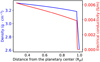 |
Fig. 1 Electrical conductivity and density profiles for a Moon-sized, Moon-mass body. The density profile was calculated using the code CHIC (Noack et al. 2016), and the electrical conductivity profile follows that of Yoshino & Katsura (2013). |
2.4 Thermal evolution model
To investigate the influence of induction heating on the Moon-sized body, we modelled its interior, long-term thermal evolution using the mantle convection code CHIC. The model mostly follows the simulations outlined in Noack et al. (2017), by using a 2D regional spherical annulus with reflective side boundaries as model geometry. Thermodynamic properties are taken from the interior structure model described in Sect. 2.3. As an initial temperature profile, we assumed that the temperature increased from 300 K at the surface to 1500 K at the bottom of the lithosphere, which we assumed to be 100 km thick initially. Below the lithosphere, assuming convection in the silicate mantle, the temperature increases adiabatically with depth; due to the low pressure increase within the mantle, temperatures increase only by 60 K over the entire mantle of more than a 1500 km thickness. At the core-mantle boundary, we assumed an initial temperature of 2000 K, which corresponds to a super-heated core. Our assumptions are based on the values typical for the Moon. Even though we concentrate here on modelling the thermal evolution of the mantle, we considered that the core cools over time due to heat flowing into the mantle. For simplicity, we did not take any possible freezing of the iron core into account. In addition to induction heating of the mantle, we also took heating by radioactive sources into account, which we assumed to be Earth-like and which decrease over time due to radiogenic decay (Schubert et al. 2001). For planets on close-in and eccentric orbits or with non-zero obliquity, strong additional heating can occur due to tidal deformations, as is the case for Jupiter’s moon Io. However, in the case of the system considered here, the timescales for tidal circularization and tidal locking are between 10 and 1000 yr, so rocky planets will be synchronized and circularized with zero obliquity very quickly (Agol 2011). Furthermore, any significant eccentricity would result in quick fragmentation of the bodies (Brown et al. 2017). Veras et al. (2017) also show that rocky differentiated bodies with moderate bulk densities of 3–4 g cm−3 on orbits with small eccentricities e < 0.1 can remain intact, even though they can sometimes lose mass from their mantles. Nonetheless, debris discs around WDs are often eccentric. Bodies on eccentric orbits would be additionally heated by tidal heating, which would be an additional energy source that could heat and contribute to melting the mantle. Taking heating into account would certainly not decrease the melt fractions, but only lead to earlier melting and higher degrees of melting.
Heating of the mantle or convection of hot material from the core-mantle boundary to the upper mantle regions leads to (partial) melting. Induction heating generates enough heat to melt large fractions of the mantle of our test planet, which cannot easily be modelled with a conventional convection code. To obtain a simple estimate of how much of the mantle would be molten, we used a simpler model. To this end, we traced which parts of the mantle would be molten by comparing the evolving temperature profile to the minimum and maximum melting temperature in the mantle (taken from Noack et al. 2017). We took neither any redistribution of the melt nor any latent heat effects from melting or crystallization of melt into account.
However, we mimicked an increased heat flow in molten regions following Golabek et al. (2011, 2014), while using a solid mantle convection model to determine the general planet heating and cooling over time. This allowed us to obtain initial insight into the amount of melting induced by induction heating and the overall heat flow evolution without the numerical complexities needed to model a mixed solid and molten mantle.
According to Golabek et al. (2011, 2014), the main effects of a magma layer on the long-term thermal evolution of the mantle manifest themselves in orders of magnitude lower viscosity and in reduced density. The effective density of a partially molten region in the interior ρeff was determined by the local melt fraction F, the local solid mantle density ρsol, and the reference melt density ρmelt as

where we set ρmelt = 3000 kg m−3 (averaged value from Lesher & Spera 2015). The effective viscosity in a molten region can be described based on Pinkerton & Stevenson (1992) as
![Mathematical equation: $ {\eta _{{\rm{eff}}}} = {\eta _{{\rm{sol}}}}\exp \left\{ { - F\left[ {2.5 + {{\left( {{F \over {1 - F}}} \right)}^{0.48}}} \right]} \right\}, $](/articles/aa/full_html/2023/09/aa45225-22/aa45225-22-eq4.png) (3)
(3)
where ηsol is the viscosity of solid silicates. To avoid errors in the numerical model for low-viscosity convection in molten regions, we set a lower viscosity cutoff at ηnum = 1016 Pa·s, that is, lower than the viscosity of Earth’s asthenosphere, which is a low-viscosity layer beneath the lithosphere of Earth’s mantle. This is assumed to be due to local melt intrusions, while in reality molten regions have a several orders of magnitude lower viscosity (Bottinga & Weil 1972; Liebske et al. 2005).
In regions with a high melt fraction, the effective local viscosity might become lower than the numerical cutoff viscosity value. Thus, we used ηconv in our convection models, defined as
 (4)
(4)
to constrain the effective viscosity to values above ηnum. To treat the strongly increased thermal flux in those regions where the cutoff viscosity is reached, we scaled up the local thermal conductivity following Golabek et al. (2011, 2014). We define the scaled thermal conductivity kmelt,scaled as
 (5)
(5)
where kmelt is the thermal conductivity of melts (with a value of 2 Wm−1 K−1; Henning et al. 2009; Dobos & Turner 2015), and ηmelt is the viscosity of melts (value of 3.31 Pa·s considered in our simulations, from Bottinga & Weil 1972).
The local effective thermal conductivity that we finally employed in our mantle convection simulations is then given as
![Mathematical equation: $ {k_{{\rm{eff}}}} = {k_{{\rm{sol}}}}\exp \left\{ {F\left[ {\ln \left( {{k_{{\rm{melt,scaled}}}}} \right) - \ln \left( {{k_{{\rm{sol}}}}} \right)} \right]} \right\}, $](/articles/aa/full_html/2023/09/aa45225-22/aa45225-22-eq7.png) (6)
(6)
where the solid mantle thermal conductivity ksol was calculated following Tosi et al. (2013).
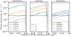 |
Fig. 2 Energy release rate inside the mantle of a planet orbiting a WD with a dipolar field of 13 MG. A magnetic field variation arises due to an inclination of the stellar magnetic dipole with respect to the stellar rotation axis. From left to right, the pictures illustrate the influence of the orbital distance (assuming a stellar inclination of 20° and a stellar rotation period of 2 h), stellar inclination (assuming an orbital distance of 0.01 au and a stellar rotation period of 2 h), and the stellar rotation periods (assuming a stellar inclination of 20° and an orbital distance of 0.01 au). The dashed horizontal line shows an average energy release inside Io of ~6.8 × 10⁻⁶ erg g−1 s−1 (Veeder et al. 2012), and the dash-dotted line shows the level of present-day Earth radiogenic heating of ~5 × 10⁻⁸ erg g−1 s−1 (Breuer 2009). |
3 Results
First, we present our calculations on induction heating inside a Moon-sized body. Then, we trace magmatic effects arising due to this heating using the interior model CHIC. Since induction heating only occurs when the magnetic field varies periodically around a planet, we assumed that the stellar magnetic field is inclined with respect to the stellar rotation axis. Therefore, the frequency of the field variation roughly equals the rotation frequency of the WD.
3.1 Induction heating of planets orbiting MWDs
We assumed a default orbital distance of 0.01 au, which is close to 1.5 times the distance to the Roche limit of approximately 0.006 au. At this distance, the typical magnetic field strength is in the range of 0.1–0.5 G for a B0 of 13 MG. This magnetic field strength would therefore be comparable to the magnetic field strength present at closer distances to WDs with weaker magnetic fields, such as WD 1145+017 (Farihi et al. 2018), but then the rocky body would be fragmented as these closer distances would lie within the stellar Roche limit. To investigate the threshold value of the total energy release and the magnetic field variation that causes changes in the interior energy budget, we modelled several additional cases of a Moon-sized body at various orbital distances.
Figure 2 presents the heating rates inside the Moon-sized body. The total heating rates for these cases are shown in Table 2. We have restricted the inclinations of the stellar magnetic dipole to ≤20°. According to our magmatic simulations, the mantle of a Moon-like object is molten within a geologically very short time as a result of induction heating if the total heating is of the order of 1019 erg s−1. Due to the limitations of our magmatic simulations, we cannot model cases with higher heating (i.e. at closer orbital distances or with higher inclinations for the stellar magnetic fields); however, it seems reasonable to assume that such bodies would be molten as well.
At 0.01 au, the maximum total energy release rates are comparable to those previously estimated for larger planets orbiting MS stars (Kislyakova et al. 2017; Kislyakova & Noack 2020). However, as we show below, such heating rates have a strong impact on the Moon-sized object considered here as a result of its smaller size.
For a Moon-sized body, electrical conductivity of the mantle is much lower than for larger planets such as the Earth, which allows the stellar magnetic field to penetrate deeper into the planet’s interior and energy to be released throughout the mantle (Fig. 2). This means that the skin depth in all cases is comparable to or even exceeds the body’s size. Due to this fact, a magnetic field that penetrates the conducting body orbiting a WD declines very slowly, which leads to energy release being distributed throughout the mantle, as one can see from various cases presented in Fig. 2. This is quite different from larger planets, where the energy release is mostly concentrated within a relatively thin layer near the planet’s surface, assuming typical stellar rotation periods and planetary orbital periods (Kislyakova et al. 2018; Kislyakova & Noack 2020). This has very important implications for the applicability of our results to WDs with different rotation periods and bodies orbiting them at various orbital distances. The right panel of Fig. 2 illustrates the influence of different stellar rotation periods on the distribution of the energy release inside the planet. One can see that apart from the obvious difference in the magnitude of the heating, the shape of the energy release stays mostly the same, only slowly declining with increasing depth. This is in contrast to the results of Kislyakova et al. (2018) obtained for larger bodies. For Earth-sized or larger planets, electrical conductivity profiles have different shapes due to the presence of different minerals and higher pressures in their mantles. This leads to high electrical conductivities that prevent a variable magnetic field from penetrating deep into the planet’s mantle. Therefore, energy release is concentrated into a narrow shell in the upper mantle directly underneath the crust. Due to melt migration, it can be expected that energy released in this region of the mantle can very efficiently drive volcanic activity due to low pressures at these depths (Kislyakova & Noack 2020).
Unlike larger planets, a Moon-sized body shows the same degrees of melting for a given heating rate assuming a realistic rotation period of the host star even as short as 2 h. Therefore, our results for a given heating rate can be applicable to a Moon-sized object orbiting a WD at any orbital distance and with any rotation rate. They can even be generalized to moonlets orbiting MS stars, as long as the heating rates inside these objects are comparable. One can calculate induction heating in a simplified way using the formula for the weak skin effect in a spherical object with a constant electrical conductivity, but we note that such simplified estimates yield imprecise results for real celestial bodies (see Appendix A).
Figure 3 illustrates the dependence of the total energy release inside the planet on the orbital distance. Since we assumed that the magnetic field declines with distance as R−3, one can see a very steep decline in the heating rate with increasing distance to the MWD. In Fig. 3 one can also see a sharp decline in the total energy release at the co-rotation point, that is, at an orbital distance where the planet’s orbital frequency equals the star’s rotation frequency. Energy release vanishes near the co-rotation point as the magnetic field variation frequency becomes very low, which is basically the case of a conducting body embedded into a constant non-varying magnetic field, which does not cause any energy release.
3.2 Influence on interiors and degree of melting
To determine the effect induction heating has on the evolution of a Moon-sized body around a MWD, we ran example simulations with the mantle convection code CHIC (Noack et al. 2016). The model setup is described in Sect. 2.4. As mentioned above, we allowed temperatures to rise above the minimum melting temperature without extracting melt or taking any latent heat consumption due to melting into account. Here and below, the minimum melting temperature specifies the temperature below which a material is completely solid. The maximum melting temperature specifies the temperature above which a material is completely liquid.
The left panel of Fig. 4 shows the degree of mantle melting as well as the mantle-averaged temperature over time for the different inclinations shown in Fig. 2. The right panel of the same figure shows the influence of different orbital distances on the mantle melting and the resulting temperature. If the temperature reaches or oversteps the maximum melting temperature, the degree of melting would be 100%. For temperatures below the minimum melting temperature, the degree of melting is zero.
The top row in the left panel shows the reference simulation without induction heating. Due to the release of radiogenic heat and cooling of the core, the average mantle temperature increases to 1715 K after 1.9 Gyr of thermal evolution. At this time, the mantle-averaged melting degree reaches 47%. Even so, the maximum melting degree is at 78% at that time, which means that even though melt can dominate locally, silicate crystals still exist in the magma. Despite that, the heat transport is dominated for a short time by melt and not by crystals. Since we accommodated for efficient cooling in the magma by including an effective, melt-solid-averaged viscosity and density, as well as a melt-increased thermal conductivity, the mantle cools efficiently until most of the interior is completely solid after 10 Gyr of thermal evolution. At that time, the average melt fraction drops to 1.3%, and the maximum local value goes down to 14%.
The left panel of Fig. 4 shows the increasing influence of induction heating for inclinations between 5 and 20°. For each case, the maximum melting temperature was locally reached, showing the immense energy release in the interior of the planet. For all considered inclinations, the thermal evolution of the interior is similar. The average temperature rose up very rapidly until a stable value within the first ~l Gyr was reached. In all these cases with non-zero inclination, the induction heating counterbalances the cooling in the interior. The average melt fraction of the mantle follows the behaviour of the average mantle temperature: the melt fraction grows and reaches a maximum value within a similar time frame. Even for the strongest induction heating (for inclinations of 20°), the mantle is not entirely molten to 100%, since the surface temperature was fixed at 300 K, enforcing a stagnant lid on top of the mantle. Without this fixed boundary condition, it is likely that average melting degrees would reach higher fractions.
Once the maximum average temperature and melt fraction values are reached, their values remain largely steady with time, with only a very minor reduction after 10 Gyr. Since the strong interior heating is balanced by a strong cooling, a quasi-steady-state is reached (thermostat effect). For all these cases, the average temperature decreases by ~ 10–20 K after its maxima, while the average melt fraction decreases only by a few percent (2-4%). In all cases, the mantle contains completely molten regions (local maximum melt fraction values of 100%) throughout the entire time evolution.
Regardless of the similarities in the evolution of all cases with non-zero induction heating, there are modest differences between the cases. For larger inclination angles, the maximum average temperature and melt fraction are reached earlier (at 1.2 Gyr and at 0.3 Gyr for inclination angles of 5 and 20°, respectively). Larger inclination angles cause stronger induction heating, and thus the average temperature and melt fraction values are slightly higher. These differences are minor, of only ~50 K in the average temperature between the cases with an inclination of 5 and 20°, and of a few percent in the average mantle melt fraction.
When comparing the case with a 0° inclination angle and those with non-zero inclination, the differences in the average mantle temperature and melt fraction are severe. The temperature differences are ~ 150–200 K at their respective peak and hundreds of Kelvin in subsequent stages, while average melt fraction differences are about 25–30% at their respective maxima. Induction heating keeps the mantle of the planet partially molten over time. The average melt fraction in the considered cases of 5, 10, 15, and 20° inclination angles is higher than the value at which the behaviour transitions from solid-like to a low-viscosity magma ocean with suspended crystals.
The right panel of Fig. 4 illustrates the influence of the orbital distance on our results. The inclination of the stellar dipole equals 20°, and the stellar rotation period equals 2 h; although, as we have shown above in Sect. 3.1, the stellar rotation period does not have a significant influence on the interior heating distribution of the body. Therefore, these results are applicable to any case with a comparable overall heating rate. One can see that the threshold heating value, which still significantly influences the thermal evolution of the Moon-sized body, is approximately 2 × 10¹⁸ erg s−1. For a stellar magnetic field of 13 MG, this corresponds to an orbital distance of 0.02 au or a magnetic field variation around the planet of 0.05 G. For a WD with a lower magnetic field and/or a different inclination of this field, the equivalent orbital distance can be calculated using Eq. (1). Comparing Figs. 2 and 4, we can conclude that for a Moon-sized body, the threshold average heating value that significantly influences the evolution by increasing the degree of melting and raising the mantle temperatures for a geologically significant time is comparable to the average heating rate in the modern-day Earth.
We assumed that the energy that was released due to induction heating was extracted from the orbital motion. Kislyakova et al. (2018) and Bromley & Kenyon (2019) have considered the time it takes to degrade the orbit of large planets orbiting MS stars due to induction heating by comparing total energy released per second to the total orbital energy. Here, if we compare the total energy release in our most extreme case of 20 degree inclination at the orbit of 0.01 au to the total orbital energy of −(GMplMst/Rorb − GMplMst/Rroche) ~ 1040 erg, we can see that the orbital drag due to this mechanism is negligible for the cases we have considered.
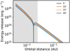 |
Fig. 3 Total energy release inside a Moon-sized planet orbiting a WD at various orbital distances. Energy release was determined by the inclination of the stellar dipole axis. The shaded area marks the region inside the Roche limit of approximately 0.006 au. One can see the co-rotation point at around 0.003 au, where induction heating is not efficient. For a short stellar rotation period of 2 h, the co-rotation region is inside the Roche limit; however, for longer rotation periods, it is located further from the star. |
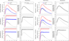 |
Fig. 4 Magmatic simulations for the heating rates shown in Fig. 2. Blue lines represent the fraction of molten mantle in percent, averaged over the entire mantle from the core-mantle boundary to the surface of the planet, while the red lines show the maximal occurring local degrees of melting. Left panel: reference simulation without induction heating shown in the first row, followed by different inclination angles of 5° and 20° in the subsequent rows. The behaviour of 10° and 15° curves is qualitatively similar to the 5° and 20° cases. The first column illustrates the maximum and average degree of melting in the mantle, and the second column shows the average mantle temperature depending on time. On the plots that include induction heating, the grey dashed line shows the curve without induction heating for comparison. Right panel: same as for the other panel, but for different orbital distances. At orbital distances larger than 0.025 au, induction heating does not significantly influence the thermal evolution. The x-axes show time in Gyr. |
4 Influence on observability
We have shown that Moon-sized bodies in close orbit around strong MWDs have a high probability of having molten mantles due to induction heating. Although our results have been obtained for a body orbiting at 0.01 au from a highly magnetized WD, they can be extrapolated to other objects orbiting very close to a star with a much weaker magnetic field. We did not consider the influence of tidal heating on the planet’s mantle, but it should be negligible for planets on circular orbits in the equatorial plane of their stars.
From observations of Solar System bodies, especially Io, we know that even small bodies with molten mantles exhibit significant volcanic activity (Peale et al. 1979). Io mainly ejects S+ and O+ ions at rates of ~2 × 1028 s−1 (Thomas et al. 2004). In addition to SO2, millimetre wavelength observations also indicate the presence of Na-, Cl-, and K-bearing volatiles, H2S, and H2 (Schaefer & Fegley 2005). On the Moon, the main outgassed elements during its active volcanic periods were H, O, C, Cl, S, and F, with the most abundant molecules being CO, H2, H2S, COS, and S2 (Renggli et al. 2017).
In general, the composition of the outgassed volatiles depends on the body’s composition, redox state of the mantle, surface pressure, and possibly other factors (e.g. Gaillard & Scaillet 2014; Katyal et al. 2020). On Earth and possibly on Mars, the gases released by volcanoes are more oxidized in comparison to the Moon or Io (Renggli et al. 2017). The exact composition and properties of the mantles of planets orbiting WDs are not clear. Nonetheless, the observed pollution of several WDs is in agreement with Earth-like fugacities (measures of rock oxidation that influence planetary structure and evolution) and general geochemistry of engulfed planets (Doyle et al. 2019). Therefore, one can possibly expect an environment and outgassing somewhat similar to those of Io or the Moon.
In addition to gas, volcanoes are known to produce significant amounts of dust. The released material becomes ionized and can be detected along the body’s orbit (Brown & Bouchez 1997; Kislyakova et al. 2019). Observations confirm at least some WDs being obscured by dust (e.g. Farihi et al. 2017; Karjalainen et al. 2019). Induction heating could be an additional factor possibly leading to copious dust production.
The ultraviolet (UV) wavelength band, particularly the far-UV (about 912–1700 Å), contains several strong resonance lines of abundant elements, including H, C, O, and S, which are among the main outgassed elements. Following Kislyakova et al. (2018), absorption signatures of these elements entailed in the planetary exosphere resulting from the outgassing might be detectable during transit with the HST or more likely with future facilities with UV capability, such as WSO-UV (Boyarchuk et al. 2016) or LUVOIR/Habex (The LUVOIR Team 2019).
If a planet’s orbit is inclined or eccentric, then tidal heating also becomes important. A pre-existing magma ocean or even a magma ‘slush’ layer in the planet’s interiors can completely change the tidal response of the body (Tyler et al. 2015), even if the orbit is quickly circularized. Once the orbit’s eccentricity and obliquity are damped, tidal heating becomes negligible, and one of the remaining powerful heating sources is induction heating due to an inclined stellar dipole.
5 Discussion
Bromley & Kenyon (2019) previously considered the influence of electromagnetic induction on thermal and orbital evolution of asteroids orbiting various stellar hosts including WDs. They show that induction effects can be strong enough to raise the temperatures inside asteroids and small planets above the maximum melting temperature. In addition to that, their results indicate that magnetic interactions can lead small bodies spiraling inwards to be eventually torn apart by tidal forces and to contribute to the observed pollution. If stellar rotation is taken into account, then bodies orbiting WDs cannot only spiral inwards, but also outwards, if the magnetic field lines are moving faster than the body’s orbital speed and thus transferring momentum to the orbiting body (Laine et al. 2008). Although effects on orbital dynamics can be significant for short-period planets close to the Roche limit, they are less important further away from the star. In this article, we do not take the effects of magnetic induction on orbital dynamics into account. Unlike Bromley & Kenyon (2019), who used an analytical approach to calculate the temperature rise in an asteroid, here we use a numerical model tracing the temperature evolution and formation of magma oceans in planetary interiors, and we also consider larger bodies.
To understand how temperatures and melt volumes change over time due to induction heating, we used a simple convection model for a solid mantle. Such a simplification did not allow us, for example, to model melt migration, the evolution of a crustal layer, volatile degassing processes, or the redistribution and re-crystallization of molten material in general. We acknowledge that the continued long-term thermal evolution of the interior could differ when taking the melt redistribution in our model into account, for example via a two-phase flow approach. Especially cooling of the interior would be expected to be stronger when accurately modelling the melt production and distribution towards the surface, similar to the heat-pipe model, where cooling of the mantle by sinking of cold surface material due to overlying crust formation is considered (Moore & Webb 2013).
However, the main aim of our study was to investigate whether large fractions of the interior would be molten at different time steps. We first estimated the amount of produced melt depending on local temperatures as already done in other mantle evolution studies (e.g. Ziethe et al. 2009). Similar to the approach of Golabek et al. (2011, 2014), we mimicked the increased heat flow through molten regions by choosing an increased, effective thermal conductivity for magma ponds or magma oceans, as well as a reduced viscosity and change in density upon melting. Even though this will not give us the full picture of the long-term thermal and chemical evolution of the mantle, a more complex model is beyond the scope of this study.
In general, we assumed a rather hot initial temperature profile with a super-heated core, leading to strong heating and melting of the mantle during the first billion years. Using lower initial temperatures, as was done in Ziethe et al. (2009), would lead to lower melt fractions in the reference case, where no induction heating was assumed. However, this would not change the melt fractions for the cases with induction heating, as can be seen by the dramatic increase in the average mantle temperatures in Fig. 4 for inclinations of 5° or higher. Furthermore, we took neither melt redistribution to the surface and the consecutive cooling of the mantle into account (Moore & Webb 2013), nor partitioning of radiogenic heat sources into melt and thus crust, which would further affect the long-term thermal evolution of the planet (Laneuville et al. 2013). It is therefore not surprising that, with our model, we do not reconcile with the observed thermal and magmatic evolution of the Moon or Io, despite using a similar composition and measurements for our model planet.
One of the limitations of our model consists in not taking the influence of the melt fraction on the electrical conductivity profile into account. In general, molten rocks have higher electrical conductivities (Yoshino et al. 2010). A magnetic field cannot penetrate as deep into the mantle of a body with a higher conductivity, which would lead to energy release concentrated closer to the planet’s surface and, in general, to lower total energy release (although the exact amount of total energy release can vary depending on other parameters such as the magnetic field variation frequency). It is however very likely that mantles already molten by induction heating would stay molten.
Our results can be generalized for bodies comparable in size to the Moon orbiting different types of stars. For MS stars, the magnetic field variation at the planet’s orbit can be calculated following Kislyakova et al. (2017). For WDs, one can use Eq. (1). After that, one can use a simple analytical formula to crudely estimate induction heating in a conducting sphere assuming a weak skin effect case (see Appendix, Eq. (A.2)). As we have shown above, for values exceeding 2 × 10¹⁸ erg s−1, one can expect elevated interior temperatures and outgassing from the planet’s interiors. The results of Eq. (A.2) most closely represent the results of the more complicated model that calculates induction heating in multiple shells assuming the average electrical conductivity of the body to be 0.005 S m−1. However, this formula calculates the heating rates approximately, as it does not account for the heat distribution in the interiors, and it cannot be used for larger planets where the weak skin effect assumption breaks down.
In addition to large Moon- or planet-sized bodies, small asteroids are also present in large numbers in debris discs. As a simple test, we also calculated induction heating for two small asteroids with radii of 10 and 20 km. For 10 and 20 km bodies, we obtained average heating values of ≈5 × 10⁻¹⁰ erg g−1 s−1 (5 × 10⁻¹⁴ Wkg−1) and ≈1.9 × 10⁻⁹ erg g−1 s−1 (1.9 × 10⁻¹³ W kg−1), respectively. We assumed that these bodies orbit at 0.01 au around a MWD with a field strength of 13 MG and that they have a uniform electrical conductivity of dry rocks of 107 CGS (or ≈10−3 S m−1). We also assumed that the inclination of the stellar dipole is 20°.
Since our interior model is not designed to calculate melting and desiccation of such small objects, we qualitatively compared our results to those by Lichtenberg et al. (2019, their Fig. 1), who studied the volatile loss from minor bodies due to 26Al heating during planet formation. Although Fig. 1 of Lichtenberg et al. (2019) presents volatile loss depending on 26Al abundance, we were able to recalculate these values into Watts per kilogram (T. Lichtenberg, priv. comm.). According to Lichtenberg et al. (2019), a planetesimal with a radius of 10 km desiccates if the average heating rate reaches 10−7−4 × 10⁻⁷ W kg−1; whereas, for a planetesimal with a larger radius of 20 km, the average heating rate of 5 × 10⁻⁸−2 × 10⁻⁷ W kg−1 is sufficient to desiccate it. One should take this comparison with caution, because little is known about the volatile content of asteroids orbiting WDs. Nonetheless, these values are orders of magnitude above the induction heating values presented above. Therefore, under these assumptions, induction heating likely cannot be a significant contribution to volatile loss from minor bodies.
However, this result changes if we consider bodies on close orbits. For asteroids orbiting at 0.001 au, the heating rates reach ≈1.4 × 10⁻² erg cm−2 s−1 (1.4 × 10⁻⁶ Wkg−1) and ≈5.8 × 10⁻² erg cm−2 s−1 (5.8 × 10⁻⁶ W kg−1) for 10 and 20 km bodies, respectively. In addition to that, induction heating becomes approximately two orders of magnitude stronger, if we assume the electrical conductivity of molten rocks to be 2−5 S m−1. Therefore, we can conclude that induction heating can be an additional powerful source of volatiles outgassing for small bodies when they spiral in before being engulfed by the WD. Even though these values are much lower than the energy received by the asteroids from stellar irradiance, energy released inside them can drive much more efficient outgassing. Since the orbital distance of 0.001 au is within the Roche lobe of WDs, it is likely that such minor bodies would be fragmented even further by tidal forces.
Our results for small bodies are in general agreement with the conclusions by Bromley & Kenyon (2019), who have also studied the effects of magnetic fields on small asteroids. According to Bromley & Kenyon (2019), induction heating is efficient for bodies on very tight orbits of 0.005 au and less. In addition to that, a slightly larger size of the body is necessary to prevent heat loss that is too rapid due to heat radiation. Bromley & Kenyon (2019) also considered the influence of magnetic induction on orbital dynamics; however, for bodies orbiting at 0.01 au, magnetic forcing is likely negligible.
6 Conclusions
We have considered the influence of electromagnetic induction heating on Moon-sized bodies orbiting strongly magnetized WDs. According to our results, even relatively small inclinations of the stellar dipole lead to significant heating and melting of the planet’s interiors. For every case considered where induction heating exceeded the threshold value of 2 × 10¹⁸ erg s−1, temperatures and melt fractions in the interior remain high over time, with much larger values than observed for the case without induction heating. With average melt fractions of ≳70%, the mantle would undergo a magma ocean-like behaviour. Although we did not model the eruption and outgassing directly, as we know from Solar System bodies, the presence of a significant melt fraction leads to significant volcanic activity with volcanoes producing gas and dust. Due to the weak gravity of Moon-sized bodies, these materials can be quickly lost to space and be distributed along the orbit of the body, as is the case for Io (Kislyakova et al. 2019). However, formation of a thin, continuously replenished atmosphere is also not excluded. Our findings therefore provide an additional confirmation for a likely presence of volcanically produced materials around WDs, which could be an important factor powering the pollution observed in the atmospheres of many WDs. According to our results, generally, induction heating is less important for small asteroids orbiting WDs, although it can be important under some conditions (very tight orbits and high electrical conductivities).
Acknowledgements
We thank the anonymous reviewer for constructive comments that helped to improve the manuscript considerably. We sincerely thank Dr. Tim Lichtenberg for a discussion regarding desiccation of small asteroids. K.K. and M.G. acknowledge support by the Austrian Research Promotion Agency (FFG) Project 873671 ‘SmileEarth’. G.V. was supported by the Government and the Ministry of Education and Science of Russia grant no 075-15-2022-262 (13.MNPMU.21.0003). L.N. and E.S. acknowledge support by the German Research Foundation (DFG) for project NO 1324/6-1 funded within the Priority Programme SPP1992 ‘Exploring the Diversity of Extrasolar Planets’. The calculations of induction heating presented in this article were performed using Python, NumPy, and SciPy.
Appendix A
We present a simplified way to calculate induction heating in a spherical body for the cases of a weak and strong skin effect. These formulas can be obtained based on Maxwell’s equations using appropriate boundary conditions. These formulas do not yield precise results for large celestial bodies, because differentiated bodies have electrical conductivities that vary with depth depending on the local mineral composition. However, these formulas can be used as a simple approximation. Here and below, all formulas are given in CGS units.
Electrical conductivity along the magnetic field’s amplitude and variation frequency determines the magnitude of induction heating. Electrical conductivity together with the period of the magnetic field change determine the skin depth, δ, which is the penetration depth of the electromagnetic field into the conducting medium. At the depth δ, the amplitude of the external magnetic field decreases by a factor of e. In an approximation of a well conducting medium (4πσ ≫ ϵω), which is applicable for the parameter range considered in this work, the skin depth is given by  , where c is the speed of light, σ is the electrical conductivity of the medium, μ is the magnetic permeability, e is the permittivity (one can assume μ = ϵ = 1, see Kislyakova et al. 2017), and ω is the frequency of the field change. Both the depth and magnitude of the maximal heating depend on the skin depth. For the strong skin effect case, the skin depth is much smaller than the radius of the body, and the maximum heating occurs close to the surface and is confined to shallow surface layers. In the weak skin effect case, the skin depth is comparable to or larger than the radius of the body, and thus the field can penetrate deep into the planetary mantle, so that the energy release occurs everywhere in the body. For the Moon-sized bodies considered here, the formalism for the weak skin effect case is applicable even for the shortest considered stellar rotation period of 2 h. For larger planets, the strong skin effect case is relevant (Kislyakova et al. 2017; Kislyakova & Noack 2020).
For the strong skin effect case, the total energy release Q inside the body can be calculated as follows:
 (A.1)
(A.1)
where ∆B is the magnetic field in the planet’s vicinity calculated according to Eq. 1 for WDs and in a slightly more complicated way for MS stars (see Kislyakova et al. (2017) for the exact formalism).
For the weak skin effect case relevant for Moon-sized objects, the total energy release can be approximated by the formula
 (A.2)
(A.2)
One can use Eq. A.2 to estimate the total energy release inside a Moon-sized body for a quick comparison to the threshold energy release of 2 × 10¹⁸ erg/s, which we have estimated using magmatic simulations. For Moon-sized objects, Eq. A.2 usually yields a result within a factor of two compared to the more complex models, if one assumes an average conductivity based on Fig. 1. Fig. 1 shows conductivity values in S/m, which should be converted to CGS units to use in Eqs. A.2 and A.1, with the conversion factor of 1 S m−1 = 8.98755224 × 10⁹ CGS.
References
- Agol, E. 2011, ApJ, 731, L31 [Google Scholar]
- Bagnulo, S., & Landstreet, J. D. 2019, A&A, 630, A65 [NASA ADS] [CrossRef] [EDP Sciences] [Google Scholar]
- Bagnulo, S., & Landstreet, J. D. 2021, MNRAS, 507, 5902 [NASA ADS] [CrossRef] [Google Scholar]
- Berdyugin, A. V., Piirola, V., Bagnulo, S., Landstreet, J. D., & Berdyugina, S. V. 2022, A&A, 657, A105 [NASA ADS] [CrossRef] [EDP Sciences] [Google Scholar]
- Bespalov, P. A., & Zheleznyakov, V. V. 1990, Sov. Astron. Lett., 16, 442 [NASA ADS] [Google Scholar]
- Bottinga, Y., & Weil, D. F. 1972, Am. J. Sci., 272, 438 [NASA ADS] [CrossRef] [Google Scholar]
- Boyarchuk, A. A., Shustov, B. M., Savanov, I. S., et al. 2016, Astron. Rep., 60, 1 [NASA ADS] [CrossRef] [Google Scholar]
- Breuer, D. 2009, Landolt Börnstein, 4, 323 [Google Scholar]
- Brinkworth, C. S., Burleigh, M. R., Lawrie, K., Marsh, T. R., & Knigge, C. 2013, ApJ, 773, 47 [NASA ADS] [CrossRef] [Google Scholar]
- Bromley, B. C., & Kenyon, S. J. 2019, ApJ, 876, 17 [NASA ADS] [CrossRef] [Google Scholar]
- Brown, J. C., Veras, D., & Gänsicke, B. T. 2017, MNRAS, 468, 1575 [NASA ADS] [CrossRef] [Google Scholar]
- Brown, M. E., & Bouchez, A. H. 1997, Science, 278, 268 [NASA ADS] [CrossRef] [Google Scholar]
- Cunningham, T., Wheatley, P. J., Tremblay, P.-E., et al. 2022, Nature, 602, 219 [NASA ADS] [CrossRef] [Google Scholar]
- Dobos, V., & Turner, E. L. 2015, ApJ, 804, 41 [NASA ADS] [CrossRef] [Google Scholar]
- Doyle, A. E., Young, E. D., Klein, B., Zuckerman, B., & Schlichting, H. E. 2019, Science, 366, 356 [NASA ADS] [CrossRef] [Google Scholar]
- Faedi, F., West, R. G., Burleigh, M. R., Goad, M. R., & Hebb, L. 2011, MNRAS, 410, 899 [NASA ADS] [CrossRef] [Google Scholar]
- Farihi, J., von Hippel, T., & Pringle, J. E. 2017, MNRAS, 471, L145 [NASA ADS] [CrossRef] [Google Scholar]
- Farihi, J., Fossati, L., Wheatley, P. J., et al. 2018, MNRAS, 474, 947 [NASA ADS] [CrossRef] [Google Scholar]
- Ferrario, L., de Martino, D., & Gänsicke, B. T. 2015, Space Sci. Rev., 191, 111 [Google Scholar]
- Fossati, L., Bagnulo, S., Haswell, C. A., et al. 2012, ApJ, 757, L15 [NASA ADS] [CrossRef] [Google Scholar]
- Gaillard, F., & Scaillet, B. 2014, Earth Planet. Sci. Lett., 403, 307 [Google Scholar]
- Gänsicke, B. T., Schreiber, M. R., Toloza, O., et al. 2019, Nature, 576, 61 [Google Scholar]
- Gissinger, C., & Petitdemange, L. 2019, Nat. Astron., 3, 401 [NASA ADS] [CrossRef] [Google Scholar]
- Golabek, G. J., Keller, T., Gerya, T. V., et al. 2011, Icarus, 215, 346 [NASA ADS] [CrossRef] [Google Scholar]
- Golabek, G. J., Bourdon, B., & Gerya, T. V. 2014, Meteor. Planet. Sci., 49, 1083 [NASA ADS] [CrossRef] [Google Scholar]
- Guenther, E. W., & Kislyakova, K. G. 2020, MNRAS, 491, 3974 [Google Scholar]
- Henning, W. G., O’Connell, R. J., & Sasselov, D. D. 2009, ApJ, 707, 1000 [Google Scholar]
- Hollands, M. A., Tremblay, P.-E., Gänsicke, B. T., Koester, D., & Gentile-Fusillo, N. P. 2021, Nat. Astron., 5, 451 [NASA ADS] [CrossRef] [Google Scholar]
- Johnstone, C. P. 2012, PhD thesis, University of St Andrews, UK [Google Scholar]
- Jura, M., & Xu, S. 2010, AJ, 140, 1129 [NASA ADS] [CrossRef] [Google Scholar]
- Jura, M., & Xu, S. 2012, AJ, 143, 6 [NASA ADS] [CrossRef] [Google Scholar]
- Karjalainen, M., de Mooij, E. J. W., Karjalainen, R., & Gibson, N. P. 2019, MNRAS, 482, 999 [NASA ADS] [Google Scholar]
- Katyal, N., Ortenzi, G., Lee Grenfell, J., et al. 2020, A&A, 643, A81 [NASA ADS] [CrossRef] [EDP Sciences] [Google Scholar]
- Kawka, A., Vennes, S., Schmidt, G. D., Wickramasinghe, D. T., & Koch, R. 2007, ApJ, 654, 499 [NASA ADS] [CrossRef] [Google Scholar]
- Kepler, S. O., Pelisoli, I., Jordan, S., et al. 2013, MNRAS, 429, 2934 [Google Scholar]
- Khodachenko, M. L., Alexeev, I., Belenkaya, E., et al. 2012, ApJ, 744, 70 [NASA ADS] [CrossRef] [Google Scholar]
- Khurana, K. K., Jia, X., Kivelson, M. G., et al. 2011, Science, 332, 1186 [Google Scholar]
- Kislyakova, K., & Noack, L. 2020, A&A, 636, L10 [NASA ADS] [CrossRef] [EDP Sciences] [Google Scholar]
- Kislyakova, K. G., Noack, L., Johnstone, C. P., et al. 2017, Nat. Astron., 1, 878 [NASA ADS] [CrossRef] [Google Scholar]
- Kislyakova, K. G., Fossati, L., Johnstone, C. P., et al. 2018, ApJ, 858, 105 [NASA ADS] [CrossRef] [Google Scholar]
- Kislyakova, K. G., Fossati, L., Shulyak, D., et al. 2019, arXiv e-prints [arXiv:1907.05088] [Google Scholar]
- Kivelson, M. G., Khurana, K. K., Stevenson, D. J., et al. 1999, J. Geophys. Res., 104, 4609 [NASA ADS] [CrossRef] [Google Scholar]
- Laine, R. O., & Lin, D. N. C. 2012, ApJ, 745, 2 [NASA ADS] [CrossRef] [Google Scholar]
- Laine, R. O., Lin, D. N. C., & Dong, S. 2008, ApJ, 685, 521 [NASA ADS] [CrossRef] [Google Scholar]
- Landstreet, J. D., & Bagnulo, S. 2019, A&A, 628, A1 [NASA ADS] [CrossRef] [EDP Sciences] [Google Scholar]
- Laneuville, M., Wieczorek, M., Breuer, D., & Tosi, N. 2013, J. Geophys. Res.Planets, 118, 1435 [NASA ADS] [CrossRef] [Google Scholar]
- Lesher, C. E., & Spera, F. J. 2015, in The Encyclopedia of Volcanoes (Amsterdam: Elsevier), 113 [CrossRef] [Google Scholar]
- Li, J., Ferrario, L., & Wickramasinghe, D. 1998, ApJ, 503, L151 [NASA ADS] [CrossRef] [Google Scholar]
- Lichtenberg, T., Golabek, G. J., Burn, R., et al. 2019, Nat. Astron., 3, 307 [Google Scholar]
- Liebske, C., Schmickler, B., Terasaki, H., et al. 2005, Earth Planet. Sci. Lett., 240, 589 [CrossRef] [Google Scholar]
- Malamud, U., & Perets, H. B. 2016, ApJ, 832, 160 [NASA ADS] [CrossRef] [Google Scholar]
- Malamud, U., & Perets, H. B. 2017, ApJ, 849, 8 [NASA ADS] [CrossRef] [Google Scholar]
- Manser, C. J., Gänsicke, B. T., Eggl, S., et al. 2019, Science, 364, 66 [Google Scholar]
- Moore, W. B., & Webb, A. A. G. 2013, Nature, 501, 501 [NASA ADS] [CrossRef] [Google Scholar]
- Murakami, G., Yoshioka, K., Yamazaki, A., et al. 2016, Geophys. Res. Lett., 43, 12, 308 [NASA ADS] [CrossRef] [Google Scholar]
- Noack, L., Rivoldini, A., & Van Hoolst, T. 2016, Int. J. Adv. Syst. Measur., 9, 66 [Google Scholar]
- Noack, L., Rivoldini, A., & Van Hoolst, T. 2017, Phys. Earth Planet. Int., 269, 40 [CrossRef] [Google Scholar]
- Noack, L., Kislyakova, K., Johnstone, C., Güdel, M., & Fossati, L. 2021, A&A, 651, A103 [NASA ADS] [CrossRef] [EDP Sciences] [Google Scholar]
- Parkinson, W. D. 1983, Introduction to Geomagnetism (UK: Scottish AcademicPress Limited) [Google Scholar]
- Peale, S. J., Cassen, P., & Reynolds, R. T. 1979, Science, 203, 892 [Google Scholar]
- Pinkerton, H., & Stevenson, R. 1992, J. Volcanol. Geotherm. Res., 53, 47 [NASA ADS] [CrossRef] [Google Scholar]
- Putirka, K., & Xu, S. 2021, Nat. Commun., 12, 6168 [NASA ADS] [CrossRef] [Google Scholar]
- Reding, J. S., Hermes, P. J., Vanderbosch, Z., et al. 2020, ApJ, 894, 19 [NASA ADS] [CrossRef] [Google Scholar]
- Renggli, C. J., King, P. L., Henley, R. W., & Norman, M. D. 2017, Geochim. Cos-mochim. Acta, 206, 296 [NASA ADS] [CrossRef] [Google Scholar]
- Roth, L., Saur, J., Retherford, K. D., et al. 2017, J. Geophys. Res. Space Phys., 122, 1903 [Google Scholar]
- Sandhaus, P. H., Debes, J. H., Ely, J., Hines, D. C., & Bourque, M. 2016, ApJ, 823, 49 [NASA ADS] [CrossRef] [Google Scholar]
- Schaefer, L., & Fegley, B. 2005, Icarus, 173, 454 [NASA ADS] [CrossRef] [Google Scholar]
- Schubert, G., Turcotte, D. L., & Olson, P. 2001, Mantle Convection in the Earthand Planets (Cambridge: Cambridge University Press) [CrossRef] [Google Scholar]
- Shimazu, H., & Terasawa, T. 1995, J. Geophys. Res., 100, 16923 [NASA ADS] [CrossRef] [Google Scholar]
- Stephan, A. P., Naoz, S., & Gaudi, B. S. 2021, ApJ, 922, 4 [NASA ADS] [CrossRef] [Google Scholar]
- Stevenson, D. J., Spohn, T., & Schubert, G. 1983, Icarus, 54, 466 [NASA ADS] [CrossRef] [Google Scholar]
- The LUVOIR Team 2019, arXiv e-prints [arXiv: 1912.06219] [Google Scholar]
- Thomas, N., Bagenal, F., Hill, T. W., & Wilson, J. K. 2004, The Io Neutral Clouds and Plasma Torus, eds. F. Bagenal, T. E. Dowling, & W. B. McKinnon (Tucson: University of Arizona Press), 561 [Google Scholar]
- Tosi, N., Yuen, D. A., de Koker, N., & Wentzcovitch, R. M. 2013, Phys. EarthPlanet. Int., 217, 48 [CrossRef] [Google Scholar]
- Trammell, G. B., Arras, P., & Li, Z.-Y. 2011, ApJ, 728, 152 [NASA ADS] [CrossRef] [Google Scholar]
- Tyler, R. H., Henning, W. G., & Hamilton, C. W. 2015, ApJS, 218, 22 [Google Scholar]
- Ud-Doula, A., & Owocki, S. P. 2002, ApJ, 576, 413 [NASA ADS] [CrossRef] [Google Scholar]
- Vanderburg, A., Johnson, J. A., Rappaport, S., et al. 2015, Nature, 526, 546 [Google Scholar]
- Vanderburg, A., Rappaport, S. A., Xu, S., et al. 2020, Nature, 585, 363 [Google Scholar]
- Veeder, G. J., Davies, A. G., Matson, D. L., et al. 2012, Icarus, 219, 701 [Google Scholar]
- Veras, D. 2016, R. Soc. Open Sci., 3, 150571 [Google Scholar]
- Veras, D., Carter, P. J., Leinhardt, Z. M., & Gänsicke, B. T. 2017, MNRAS, 465, 1008 [NASA ADS] [CrossRef] [Google Scholar]
- Walters, N., Farihi, J., Marsh, T. R., et al. 2021, MNRAS, 503, 3743 [NASA ADS] [CrossRef] [Google Scholar]
- Weber, R. C., Lin, P.-Y., Garnero, E. J., Williams, Q., & Lognonné, P. 2011, Science, 331, 309 [NASA ADS] [CrossRef] [Google Scholar]
- Weiss, B., & Tikoo, S. 2014, Science, 346, 1246753 [NASA ADS] [CrossRef] [Google Scholar]
- Wickramasinghe, D. T., Farihi, J., Tout, C. A., Ferrario, L., & Stancliffe, R. J. 2010, MNRAS, 404, 1984 [NASA ADS] [Google Scholar]
- Willes, A. J., & Wu, K. 2005, A&A, 432, 1091 [NASA ADS] [CrossRef] [EDP Sciences] [Google Scholar]
- Yoshino, T., & Katsura, T. 2009, Phys. Earth Planet. Int., 174, 3 [CrossRef] [Google Scholar]
- Yoshino, T., & Katsura, T. 2013, Ann. Rev. Earth Planet. Sci., 41, 605 [CrossRef] [Google Scholar]
- Yoshino, T., Laumonier, M., McIsaac, E., & Katsura, T. 2010, Earth Planet. Sci.Lett., 295, 593 [CrossRef] [Google Scholar]
- Ziethe, R., Seiferlin, K., & Hiesinger, H. 2009, Planet. Space Sci., 57, 784 [NASA ADS] [CrossRef] [Google Scholar]
- Zimmer, C., Khurana, K. K., & Kivelson, M. G. 2000, Icarus, 147, 329 [NASA ADS] [CrossRef] [Google Scholar]
For context, we would like to specify that the strongest magnetic fields detected in non-degenerate stars are of the order of 10 kG on the surface; whereas, for Sun-like MS stars, typical magnetic field strengths of the dipole fields are of the order of 1–10 G.
All Tables
Heating rates and magnetic field variations ∆B for different inclinations of the stellar dipole I, orbital distances, and stellar rotation periods.
All Figures
|
Fig. 1 Electrical conductivity and density profiles for a Moon-sized, Moon-mass body. The density profile was calculated using the code CHIC (Noack et al. 2016), and the electrical conductivity profile follows that of Yoshino & Katsura (2013). |
| In the text | |
|
Fig. 2 Energy release rate inside the mantle of a planet orbiting a WD with a dipolar field of 13 MG. A magnetic field variation arises due to an inclination of the stellar magnetic dipole with respect to the stellar rotation axis. From left to right, the pictures illustrate the influence of the orbital distance (assuming a stellar inclination of 20° and a stellar rotation period of 2 h), stellar inclination (assuming an orbital distance of 0.01 au and a stellar rotation period of 2 h), and the stellar rotation periods (assuming a stellar inclination of 20° and an orbital distance of 0.01 au). The dashed horizontal line shows an average energy release inside Io of ~6.8 × 10⁻⁶ erg g−1 s−1 (Veeder et al. 2012), and the dash-dotted line shows the level of present-day Earth radiogenic heating of ~5 × 10⁻⁸ erg g−1 s−1 (Breuer 2009). |
| In the text | |
|
Fig. 3 Total energy release inside a Moon-sized planet orbiting a WD at various orbital distances. Energy release was determined by the inclination of the stellar dipole axis. The shaded area marks the region inside the Roche limit of approximately 0.006 au. One can see the co-rotation point at around 0.003 au, where induction heating is not efficient. For a short stellar rotation period of 2 h, the co-rotation region is inside the Roche limit; however, for longer rotation periods, it is located further from the star. |
| In the text | |
|
Fig. 4 Magmatic simulations for the heating rates shown in Fig. 2. Blue lines represent the fraction of molten mantle in percent, averaged over the entire mantle from the core-mantle boundary to the surface of the planet, while the red lines show the maximal occurring local degrees of melting. Left panel: reference simulation without induction heating shown in the first row, followed by different inclination angles of 5° and 20° in the subsequent rows. The behaviour of 10° and 15° curves is qualitatively similar to the 5° and 20° cases. The first column illustrates the maximum and average degree of melting in the mantle, and the second column shows the average mantle temperature depending on time. On the plots that include induction heating, the grey dashed line shows the curve without induction heating for comparison. Right panel: same as for the other panel, but for different orbital distances. At orbital distances larger than 0.025 au, induction heating does not significantly influence the thermal evolution. The x-axes show time in Gyr. |
| In the text | |
Current usage metrics show cumulative count of Article Views (full-text article views including HTML views, PDF and ePub downloads, according to the available data) and Abstracts Views on Vision4Press platform.
Data correspond to usage on the plateform after 2015. The current usage metrics is available 48-96 hours after online publication and is updated daily on week days.
Initial download of the metrics may take a while.