| Issue |
A&A
Volume 676, August 2023
|
|
|---|---|---|
| Article Number | A59 | |
| Number of page(s) | 13 | |
| Section | Astrophysical processes | |
| DOI | https://doi.org/10.1051/0004-6361/202346658 | |
| Published online | 07 August 2023 | |
Measuring spin in coalescing binaries of neutron stars that show double precursors
1
Theoretical Astrophysics, IAAT, University of Tübingen, Tübingen 72076, Germany
2
Max Planck Institute for Gravitational Physics (Albert Einstein Institute), 14476 Potsdam, Germany
e-mail: This email address is being protected from spambots. You need JavaScript enabled to view it.
3
Department of Physics, National Tsing Hua University, Hsinchu 300, Taiwan
4
Manly Astrophysics, 15/41-42 East Esplanade, Manly, NSW 2095, Australia
Received:
14
April
2023
Accepted:
19
June
2023
Abstract
Gamma-ray bursts resulting from binary neutron-star mergers are sometimes preceded by precursor flares. These harbingers can be ignited by quasi-normal modes, excited by orbital resonances, shattering the stellar crust of one of the inspiralling stars up to ≳10 s before coalescence. In the rare case when a system displays two precursors, successive overtones of either interface modes or g modes can be responsible for the overstrainings. Since the free-mode frequencies of these overtones have an almost constant ratio, and the inertial-frame frequencies for rotating stars are shifted relative to static ones, the spin frequency of the flaring component can be constrained as a function of the equation of state, the binary mass ratio, the mode quantum numbers, and the spin-orbit misalignment angle. As a demonstration of the method, we find that the precursors of GRB090510 hint at a spin frequency range of 2 ≲ ν⋆/Hz ≲ 20 for the shattering star if we allow for an arbitrary misalignment angle, assuming ℓ = 2 g modes account for the events.
Key words: gamma-ray burst: individual: 090510 / stars: oscillations / gravitational waves
© The Authors 2023
 Open Access article, published by EDP Sciences, under the terms of the Creative Commons Attribution License (https://creativecommons.org/licenses/by/4.0), which permits unrestricted use, distribution, and reproduction in any medium, provided the original work is properly cited.
This article is published in open access under the Subscribe to Open model.
Open access funding provided by Max Planck Society.
1. Introduction
Some short gamma-ray bursts (SGRBs), which are thought to originate from binary neutron-star (NS) mergers, are preceded by precursor flares with a time advance that ranges from ∼1 to ≳10 s (Troja et al. 2010; Minaev et al. 2018; Zhong et al. 2019; Wang et al. 2020). These early flashes can be caused by crust-yielding in magnetised NS members, a result of resonantly excited quasi-normal modes (QNMs; Tsang et al. 2012; Tsang 2013; Suvorov & Kokkotas 2020b; Kuan et al. 2021b). In this context, the timing of a precursor relative to the SGRB, which also depends on a jet formation and/or breakout timescale, estimates the frequency of the mode that leads to the crustal fracture. On rare occasions, more than one precursor precedes the SGRB, for which the frequencies of the two responsible modes can be acquired (e.g., Kuan et al. 2021b).
Certain details of the stellar fabric can be accessed from the QNM spectrum; for example, the interior mean density strongly correlates with the frequencies of pressure modes (Andersson & Kokkotas 1998; Krüger & Kokkotas 2020), and g modes encode microphysical temperature or composition gradients. Here we discuss a novel way to determine the spin of a NS if a double precursor event is observed. In particular, mode frequencies in a rotating NS, attributable to the pre-emissions, provide two relations between the free-mode frequencies of these two modes and the stellar spin. In scenarios where the free-mode frequencies have a constant ratio, such as for g and i modes as explained below, this additional relation then allows the spin to be inferred. In the current era of gravitational-wave (GW) astrophysics, estimating the spins of binary NSs is crucial for reducing the errors in other measurements (e.g., Ma et al. 2021; Gupta et al. 2023); for instance, the estimates of tidal deformability of GW170817 and GW190425 are sensitive to the spin priors assumed for the progenitors (Abbott et al. 2017, 2019b, 2020; Annala et al. 2018). Properties of the post-merger system, such as the gravitational waveform (Kastaun et al. 2017), the content of dynamically ejected matter (Fujibayashi et al. 2018), remnant disc mass (East et al. 2019), and the kilonova (Papenfort et al. 2022), also depend sensitively on the spins of the pre-merger stars. In addition, simultaneous knowledge of the spin and the mode frequencies can set strong constraints on the equation of state (EOS; Biswas et al. 2021). In this work we use a particular way of manoeuvring out the spin for SGRB 090510, an event preceded by two precursors occurring ∼13 and ∼0.5 s prior to the main burst (Abdo et al. 2009; Troja et al. 2010).
Section 2 of this article briefly reviews the theory of resonant shattering as a mechanism for precursor ignition, with an emphasis on g modes (though see also Sect. 4.3). Theoretical predictions based on binary formation channels are considered in Sect. 2.3, including those relevant for misalignment angles and timing considerations (Sect. 2.4). Section 3 forms the main part of the paper and demonstrates, in principle, how the timing of double precursors can constrain the spin frequency of the flarer. By exploiting the approximately constant ratio between g1 and g2 modes, and how stellar spin modifies the mode frequencies, our key result is a fitting formula (Eq. (23)) that takes tidal heating between fracture events into account (Sect. 2.5) to estimate the spin of the star assuming that it emits two precursors. A discussion on uncertainties due to a jet formation and/or breakout timescale is also presented in Sect. 3.2 for the sake of completeness. A discussion on blue and/or red kilonovae and GWs from the remnant is presented in Sect. 4. The article is summarised in Sect. 5.
2. GRB precursors via g-mode resonances
Although the definition of pre-emission in SGRBs is not uniquely given as, for instance, some authors require the waiting time to be longer than the main burst duration (Minaev et al. 2018) while others do not (Zhong et al. 2019), precursor flares have been confidently identified in rare (≲10%) cases (Wang et al. 2020). These early flares may be triggered by certain, resonantly-excited QNMs (Tsang et al. 2012; Suvorov & Kokkotas 2020b; Kuan et al. 2021b). The (linear) orbital frequencies of precursors, which are uncertain owing to a delay between the main gamma-ray burst (GRB) and the merger through a jet formation and subsequent breakout timescale, suggest that ∼100 Hz modes are promising to account for the pre-emissions; in particular, shear, interface, and g modes have attracted some attention (Tsang et al. 2012; Tsang 2013; Kuan et al. 2021b). We focus on the g-mode scenario in this article since we may accommodate double precursors by one class of modes, though a discussion about other modes is given in Sect. 4.3.
2.1. Parameterised g modes
Composition and/or temperature gradients stratify the interior of a NS, so that it may support g modes. The spectrum of these modes is determined by the ‘adiabatic index’ of the fluid perturbation relative to that of the (beta-equilibrium) background, setting the characteristic Brunt-Väisälä frequency (e.g., Reisenegger 2001). In general, the index depends on the respective Fermi energies of each particle species, most notably through the electron fraction Ye, and the temperature of the star (e.g., Haensel et al. 2002). Realistic profiles for these quantities are complicated, and depend on a number of largely uncertain aspects of the stellar interior (see Lattimer 2012, for a review). In this work, our main goal is to illustrate a method by which spin can be measured in NS–NS mergers that release two precursor flares. To this end, we work within the context of the simple, toy framework described by Kuan et al. (2021a) (see also Gaertig & Kokkotas 2009; Passamonti et al. 2009, 2021; Xu & Lai 2017), where stratification is encoded in a spatially constant but time-dependent parameter δ, defined as the difference between the (generally density-dependent) adiabatic indices of the perturbation and the background star1. More specifically, we define2
![Mathematical equation: $$ \begin{aligned} \delta (t,\boldsymbol{x}) =\left[ \frac{k^2\pi ^2}{6}\sum _x \frac{n_x(\boldsymbol{x})}{E_F^x(\boldsymbol{x})} \right] \frac{T(t,\boldsymbol{x})^2}{p(t,\boldsymbol{x})} \end{aligned} $$](/articles/aa/full_html/2023/08/aa46658-23/aa46658-23-eq1.gif) (1)
(1)
for the pressure, p, and temperature, T, where particle species x has number density nx and Fermi energy  , and the sum includes the species list (treated as being just non-relativistic n and p, for simplicity), and assume ∇jδ ≈ 0 (see Appendix A). In the time between ∼102 s before the first precursor and the merger, the composition of the star changes very little, though the temperature can evolve dramatically (e.g., Lai 1994). As such, both thermal and compositional gradients define δ(t0, x) for simulation start time t0, while only thermal gradients then contribute to the evolution of δ due to tidal effects and mode-induced backreaction (see Sect. 2.5 for more details). The shift in g-mode spectra at late times is largely attributable to heating, even though the composition gradient is the main source of stratification; some studies suggest an effective δ ≳ 0.01 for compositional stratification (e.g., Reisenegger 2009; Akgün et al. 2013).
It should be recognised therefore that the numerical estimates we provide for spin frequencies are subject to some systematic uncertainty, and do not necessarily represent realistic, astrophysical predictions. In principle, however, one could solve the relevant thermodynamic system, for a given EOS, to self-consistently identify the value of δ for a particular type of perturbation and (magneto-)hydrodynamic equilibrium. Such complications include the possible existence of superfluidity and/or a hadron-quark transition in the core, both of which lead to larger g-mode frequencies (e.g., Yu & Weinberg 2017; Jaikumar et al. 2021). We endeavour to present formulae in such a way that the reader can readily substitute alternative values, to pave the way for more realistic investigations in future.
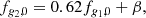
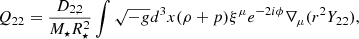
In the context of g modes, the restoring force is much weaker than that supplied by the hydrostatic pressure in the NS core, meaning that g-mode motions are suppressed in this region. The stratification in the crust then largely determines the g-mode spectrum. This was confirmed numerically in Kuan et al. (2022) for relativistic stars, who found quantitatively similar spectra for various spatially varying δ(x) profiles relative to cases with constant δ, as long as the surface values match (see Sect. 2.1 therein and Appendix A). Either way, most EOSs predict a typical value for mature NSs of δ ≳ 0.005 (Xu & Lai 2017), while the free-mode frequencies of g1 (fg1, 0) and g2 modes (fg2, 0) scale as the square root of δ, viz.,  for a parameter α depending on EOS, mode’s quantum-number, and the mass (M⋆) and radius (R⋆) of the NS (Kuan et al. 2022). In addition, they can be related via (see Fig. 1)
 (2)
(2)
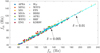 |
Fig. 1. Correlation between the frequencies of g1 and g2 modes for various EOSs and two representative values of δ (see the plot legends). For a given δ, the relations between g1 and g2 modes (Eq. (2)) are shown as bright blue lines, with the solid line representing δ = 0.005 and the dash-dot one δ = 0.01. |
for an EOS-independent parameter β ≈ 4.32 Hz. We note that, in the high-n limit, the ratio fgn + 1/fgn becomes exactly n/(1 + n) for any EOS (see expression (5.13) in Lai 1994). However, QNM frequencies of forced systems deviate from those of free systems; given a perturbing force δFμ, a frequency shift of (Unno et al. 1989; Suvorov & Kokkotas 2020b)
 (3)
(3)
is induced for Lagrangian displacement ξμ, free-mode frequency f0, mass density ρ, lapse function Φ, and metric determinant g. For centrifugal forces in stars rigidly rotating at a rate of ν⋆, we have a simple expression (see Eqs. (70) and (71) of Kuan et al. 2021a),
 (4)
(4)
for the inertial-frame frequency, f. The constant C depends on the EOS and the mode quantum numbers; the azimuthal one, m, leads to a Zeeman-like splitting of the modes (e.g., Krüger & Kokkotas 2020). As shown by Kuan et al. (2021a), rotation affects the frequencies of g1 and g2 modes to a similar extent; denoting the constant in Eq. (4) for g1 and g2 modes by, respectively, C1 and C2, for a broad set of EOSs (see the legend of Fig. 1), we find two facts about C1 and C2 for 10−3 ≤ δ ≤ 0.05: (i) Both depend only weakly on M⋆ and the EOS. (ii) The maximum difference between the value of C1 and C2 is ∼13%. (iii) The values of both are 0.11–0.12, while we note that the Newtonian approximation yields C ≃ 1/ℓ(ℓ + 1) = 0.167 for ℓ = 2 (see e.g., Vavoulidis et al. 2008).
In addition to spin-induced modulations, tidal (Kuan et al. 2021a; Yu et al. 2023) and redshift (Steinhoff et al. 2016; Zhou et al. 2023) factors also influence the mode frequency. The former effect can be taken into account by including the tidal ‘force’ within Eq. (3), though the resulting shift in g-mode frequency is less than the spin-induced one by at least three orders of magnitude for ν⋆ ≳ 1 Hz (see Sect. 5.2 of Kuan et al. 2021a). Redshift effects (that is, accounting for the fact that frequencies differ between the NS and laboratory frames) are more important, though still relatively small. Assuming a circular orbit and an equal-mass binary (q ≈ 1), the relevant redshift factor is encoded in the lapse function, which, to the leading (post-Newtonian) order and ignoring spin corrections, reads (cf. Eq. (3.6) of Steinhoff et al. 2016)
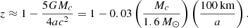 (5)
(5)
Given that the onset of g-mode resonances are typically ∼1–10 s before merger, the separation at resonance is a ≳ 100 km. As expression (5) shows, we expect a frequency shift of at most a few per cent and so neglect the effect here. By contrast, the redshift is sizeable for f-mode resonances (Steinhoff et al. 2016).
2.2. Resonant shattering
As the NSs inspiral, tidal fields induce perturbing forces that act predominantly at frequencies that are twice the orbital frequency (Zahn 1977; Tsang et al. 2012). The forced system for QNMs suggests that a particular mode will be brought into resonance when its frequency matches the forcing rate, where the mode amplitude increases rapidly until hitting a ceiling value that depends on the so-called overlap integral. After the mode leaves the resonance window, its amplitude decays by viscosity. The timescale of the dissipation is generally much longer than the rest of the life of the coalescing binary, whereas the resulted heating may change the stellar condition significantly right before merger (e.g., Kanakis-Pegios et al. 2022). In addition, the crustal strain exerted by the mode reads  , where overbar denote complex conjugation, and the stress tensor is given by (see Eqs. (22) and (23) in Kuan et al. 2021b)
 (6)
(6)
with Γ the Christoffel symbols of the background metric, whose perturbation is δg. A given mode stresses the crust at a strength that is linear in the mode amplitude to which the crust may yield if a certain threshold is met. The threshold depends on the composition, including possible impurities of the crust, and the EOS; a range of maxima have been deduced from numerical simulations, varying from 0.04 to ∼0.1 (Horowitz & Kadau 2009; Baiko & Chugunov 2018). Here we adopt σmax = 0.04, that is, crustal regions where a strain of σ ≥ σmax are set to yield. We also work with the specific von Mises breaking criterion.
During and after shattering, some energy stored in the fractured crevice(s) is transferred to nearby regions, triggering aftershocks (Duncan 1998), and to the exterior magnetic field. In the latter case, the energy deposited into (open) field lines may lead to the transient gamma-ray emissions that constitute precursor flares. These emissions are expected to have non-thermal spectra if the field strength is sufficiently strong, B ≫ 1013 G (Tsang et al. 2012). In the event that the precursor is accompanied by noticeable aftershock-induced mode(s), the light curve of the precursor may feature a quasi-periodic behaviour (Suvorov et al. 2022), such as was observed in the recent event GRB 211211A (Gao et al. 2022). This event, despite being of long duration, was also accompanied by a kilonova and thus likely resulted from a merger event. We remark therefore that the method presented here may also apply to some long GRBs with double precursors, such as GRB 190114C (in principle), for which precursors were observed 5.6 s and 2.9 s prior to the main event (Coppin et al. 2020).
2.3. Binary formation channels
Although the criterion we adopt for a crust-yielding is simply that σmax is exceeded somewhere, a number of factors complicate the overall resonant-shattering picture. Most notable for our discussion are issues related to the orientations, masses, and the EOSs of both stars. These factors hint at which star is more likely to generate precursors; for example, g modes in stars with mass ∼1.45 M⊙ couple weakly to the exterior tidal field (see Appendix of Kuan et al. 2022), and are thus incapable of producing resonant-shattering flares. In addition, the misalignment angle will in general reduce the extent to which a mode can be excited. Therefore, we may be able to deduce which star in the binary exhibits precursors if these parameters are given.
In the canonical formation channel of close binary NSs, there are two supernovae, likely of the ultra-stripped variety, separated by a timescale that is sensitive to a number of source specifics (Tauris et al. 2015, 2017; van den Heuvel 2017). Accretion by the first born from the not-yet-collapsed one can be of a disc or a wind-fed nature depending on the orbital period and Roche lobe interplay (Paczyński 1971). If a disc forms, fluid motions in the magnetically threaded disc torque the NS (e.g., Glampedakis & Suvorov 2021), gradually aligning its rotation axis with the angular momentum of the whole system while spinning it up. Wind-fed accretion is much less efficient for this purpose. The extent of alignment is therefore determined by the time separation between the two supernovae, and the nature of accretion (or its absence). The second NS will, however, not be ‘recycled’ or have its angular momentum axis oriented with that of the orbit; even relatively weak supernova kicks may arbitrarily reorient the relevant axes (cf. Tauris et al. 2017). Moreover, the coalescence will be expedited significantly if the companion is propelled towards the primary through a strong kick (see Postnov & Yungelson 2014, for a detailed discussion on the influence of natal kicks on the merger rate). In some cases, the first born NS, taken as the primary in this article, can be long-term recycled and eventually reach an aligned, possibly large spin, while the companion is relatively slow with a potentially non-negligible tilt angle (see e.g., Zhu et al. 2018; Zhu & Ashton 2020). However, if accretion is prematurely truncated by the supernova of the companion or if both stars explode roughly at the same time, one may anticipate that the binary will consist of two misaligned NSs. If the coalescence timescale turns out to be shorter than many spin-down times, the latter of which is likely controlled by magnetic braking, a system where the companion does not spin down significantly prior to coalescence could eventuate.
To summarise, at moments close to merger, the primary may rotate (comparatively) rapidly and be aligned if it has undergone long-term recycling by disc-fed accretion, while the companion may be rotating relatively rapidly only if it is kicked towards the primary. Although the magnetic energy of the primary may be depleted by (Hall-accelerated) Ohmic decay (e.g., Suvorov et al. 2016), which brakes the star while it recycles, it may still have a strong, localised field ‘buried’ under the accreted layers near the surface (e.g., Suvorov & Melatos 2020). On the other hand, globally strong fields could persist in the companion if it is kicked into the primary, especially if it settles into a ‘Hall attractor’ state (Gourgouliatos & Cumming 2014). We note, additionally, that in the event of dynamical capture, both members of the binary are also likely to be misaligned, and the companion will be regardless.
We stress that the above discussion is not meant to be an exhaustive survey on formation channel possibilities, but illustrates that a wide range of magnetic field strengths, spins, and misalignment angles are theoretically plausible. Observationally speaking, the tilt angle between the spin and the orbital angular momentum axes has been estimated for five Galactic NSs through geodetic precession and optical polarimetric measurements: (18 ± 6)° for PSR B1913+16 (Kramer 1998), < 3.2° for PSR J0737-3039A (Ferdman et al. 2013), (27 ± 3)° for PSR B1534+12 (Fonseca et al. 2014), < 34° for PSR J1756-2251 (Ferdman et al. 2014), and > 20° Her X-1 (Doroshenko et al. 2022). Four have a mild misalignment angle. Tidal activity in tilted NSs is investigated in Sect. 2.4, using these data as representative examples.
2.4. Resonance in misaligned binaries
For the reasons discussed above, it is worth investigating how the resonant-shattering procedure proceeds in cases where one or both of the binary members are misaligned. Although the QNM excitation in an aligned NS is dominated by m = 2 modes (Zahn 1977), for a misaligned NS, in general, the whole range of −l ≤ m ≤ l modes will be excited to an extent that depends on the Wigner D functions defined below (e.g., Xu & Lai 2017). Without loss of generality, we focus on a tilted primary forced by the tidal potential built by the companion. The leading-order component of potential corresponds to l = 2 and has the form
![Mathematical equation: $$ \begin{aligned}&\Phi (\boldsymbol{x},t) = -\frac{M_{c}r^{2}}{a^{3}}\left(\frac{3\pi }{10}\right)^{1/2}\nonumber \\&\qquad \qquad \times \left[e^{-2i\phi _c}Y_{22}(\theta _L,\phi _L)+e^{2i\phi _c}Y_{2,-2}(\theta _L,\phi _L)\right], \end{aligned} $$](/articles/aa/full_html/2023/08/aa46658-23/aa46658-23-eq10.gif) (7)
(7)
where Ylm denotes spherical harmonics, the numerical coefficient (3π/10)1/2 is the constant W2, ±2 used in other studies (e.g., Eq. (15) of Kokkotas & Schafer 1995), and x denotes the spatial coordinates in the inertial frame of the primary, with respect to which the phase coordinate of the companion is ϕc. Here (θL, ϕL) are the polar, and phase coordinates of the orbital angular momentum relative to the spin-axis of the primary.
In terms of the Wigner D functions, Dmm′(Θ), for tilt angle Θ made between spin and angular momentum axes, the potential (7) can be rewritten as (Lai & Wu 2006; Xu & Lai 2017)
![Mathematical equation: $$ \begin{aligned}&\Phi (\boldsymbol{x},t) = -\frac{M_{c}r^{2}}{a^{3}}\left(\frac{3\pi }{10}\right)^{1/2} \bigg [e^{-2i\phi _c}\sum _{m^{\prime }} D_{2m^{\prime }}(\Theta )Y_{2m^{\prime }}(\theta ,\phi )\nonumber \\&\qquad \qquad +e^{2i\phi _c}\sum _{m^{\prime \prime }} D_{-2m^{\prime \prime }}(\Theta )Y_{2m^{\prime \prime }}(\theta ,\phi )\bigg ], \end{aligned} $$](/articles/aa/full_html/2023/08/aa46658-23/aa46658-23-eq11.gif) (8)
(8)
where the relevant D functions read
 (9)
(9)
 (10)
(10)
 (11)
(11)
 (12)
(12)
 (13)
(13)
We see that, in contrast to the non-spinning and aligned-spinning cases, modes with m ≠ 2 will also be excited by the tidal field in misaligned NSs to different levels depending on the inclination.
It is expected that the excitation of modes with m ≤ 0 is weak relative to those with positive m since spin reduces the frequencies of the retrograde modes, giving rise to earlier excitation or even resonance, where Φ is weaker. We therefore specify ourselves to modes with m = 1 and m = 2, for which the tidal overlap is, respectively (Kuan et al. 2021a; Miao et al. 2023)
 (14)
(14)
 (15)
(15)
where the displacement ξμ is normalised such that
 (16)
(16)
We note that the fluid motion caused by a general m mode is ξμe−imϕ, and thus modes with the same l share the same displacement. Denoting the tidal overlap of an l = 2 = m mode in an aligned NS, where D2, 2 = 1 and D2, 1 = 0, as  , we have the simple scalings
 (17)
(17)
The relative strength between Q22 and Q21 is thus encoded in the associated Wigner D functions, and depends on Θ.
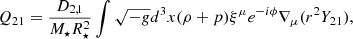
In Fig. 2 we plot D2, 2 and |D2, 1| as functions of Θ, where we see that the overlap of the m = 1 mode starts to be stronger than the m = 2 one for Θ ≳ 53.13°. We note additionally that Q21 is less than half of Q22 even when Θ ≲ 40°. Here we consider the stratification of δ = 0.012. However, we should keep in mind that the stronger overlap of m = 1 does not necessarily imply that the excitation of an m = 1 mode would be stronger than the m = 2 mode because the mode frequency of the latter is lower, implying an earlier excitation. The exact value of the minimal Θ such that the excitation of m = 1 mode is stronger (i.e. the saturation amplitude is larger) than the m = 2 one depends on the EOS, mass ratio, and the nature of modes (e.g., f, g, or i modes). Taking g1 modes for example, for binaries with total mass of 2.5 M⊙ we list in Table 1 the minimal Θ for which the m = 1 excitation in the heavier NS can exceed the extent of that of the m = 2 mode for several mass ratios between two stars q ≤ 1, some spins of the breathing star, and five EOSs. The considered EOSs are arranged in the order of softness from stiffest (left; KDE0V) to softest (right; MPA1). We see that the critical tilt angle admitting a greater dominant m = 1 is not overly sensitive to the mass ratio, though we note that the dependence is enhanced when a larger spin is considered. In addition, the critical angle is larger for softer EOSs since the g1 mode’s frequency is lower for a fixed stellar mass thus, the onsets of m = 1 and m = 2 excitations will be further separated.
 |
Fig. 2. Tidal overlap of m = 1 (red curve) and m = 2 (blue curve) modes as functions of inclination, Θ, in units of the tidal overlap of the l = 2 = m mode in an aligned NS (i.e. |

Minimum tilt angle of the heavier NS in binaries with a total mass of 2.5 M⊙, such that the m = 1 g1 mode is excited to a greater extent than the m = 2 g1 mode in the sense specified in the main text.
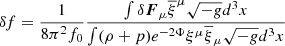
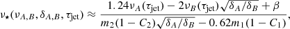
We plot in Fig. 3 the evolutions of the strain by m = 1 and m = 2 g1 modes in a NS member of an equal-mass binary as functions of the time prior to merger tp. Three cases are shown: (i) The resonance of the m = 2 mode occurs at tp = 1 s, whose strain at that moment equals σmax = 0.04 (Baiko & Chugunov 2018). (ii) Same as (i) but for the m = 1 mode. (iii) The resonance of the m = 1 mode occurs at tp = 1 s, whose saturation strain equals that of the m = 2 mode. In each of these three scenarios, the strain of m = 2 mode successfully exceeds the cracking threshold, while the m = 1 mode is not strong enough to break the crust for case (i). In the middle and bottom panels (case (ii) and (iii)), we see a 60% drop in the saturation strain of the m = 2 mode and a mild (∼25%) increase in that of the m = 1 mode by increasing the tilt angle from 30° to 80°. From Fig. 2 we know that the maximal strain of both modes will decrease monotonically as Θ ∼ 60° for a given spin. For the star considered in Fig. 3, neither mode is able to yield the crust if Θ ≳ 80°.
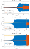 |
Fig. 3. Strain (σ) induced by m = 2 and m = 1 g1 modes (blue and red curves, respectively) of a star spinning at ν⋆ = 30 Hz (top panel) or at ν⋆ = 63 Hz (middle panel), both with Θ = 30°, and a star spinning at ν⋆ = 63 Hz with Θ = 80° (bottom panel), all as functions of t, where the merger corresponds to t = 0. The stratification is set through δ = 0.021, as relevant for the later precursor of GRB 090510 (see Sect. 3.1). The horizontal dashed lines represent the breaking threshold; σmax = 0.04 is adopted here (Baiko & Chugunov 2018). The binary is considered to be symmetric and consists of stars of masses 1.23 M⊙ with the APR4 EOS. |
2.5. Tidal heating
In addition to the alignment concern about the NS, tidal heating due to the viscous dissipation activated by mode excitations also complicates the present investigation. As described previously, the stratification is a function of time, δ(t), because of heating implying that the g-mode spectrum itself is time-dependent. In particular, Lai (1994) has shown that a non-resonantly excited l = 2 = mf mode in an aligned NS will increase the star’s temperature by (see Eq. (8.30) therein)
 (18)
(18)
which depends on the stellar radius and separation a; we remark that the subscript a here denotes the heating in aligned stars.
In the last stages of merger, f modes lead to the greatest degree of heating (∼5 times more than g modes, for instance; cf. Kuan et al. 2022) because they efficiently vibrate the entire star. While g modes actually lead to equal or even dominant heating over the life of the binary, their contribution is negligible relative to the f mode in the last ≲102 s of inspiral where our simulation applies. However, this does not necessarily imply that f-mode heating controls the stratification index in regions of the star where the g-mode eigenfunction is defined (e.g., in the crust). Even if other modes carry less overall energy, for example, they could heat the crust to a larger degree than the global f modes. This is especially true in cases where a g mode breaks the crust, which goes on to experience plastic heating (e.g., Link & Epstein 1996; Beloborodov & Li 2016). It is, in general, a difficult problem to assess and evolve the local temperature gradients that result from mode-induced perturbations, resonant or otherwise (though see Pan et al. 2020). To provide a concrete but simple example, we adopt the volume-averaged expression (18) to define how the temperature, and hence δ, evolves following the first fracture. A further study considering a more sophisticated temperature profile in the crust (e.g., Gudmundsson et al. 1982; Link & Epstein 1996; Potekhin et al. 1997) is deferred to future work.
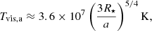
For a particular binary, we show Tvis, a as a function of time in Fig. 4. Although the f-mode excitation also modifies the orbit evolution, to estimate the heating to the leading order we adopted the well-known expression for the separation of binaries that are shrinking due to quadrupolar gravitational emission generated by the orbital motion (mode backreaction is not included), given by
 (19)
(19)
 |
Fig. 4. Temperature evolution due to heating by the viscous dissipation of f-mode excitations. Top: numerical (blue) and analytic (red; Eq. (20)) results obtained for a symmetric binary consisting of stars with 1.23 M⊙ and the EOS APR4. Bottom: ratio of the temperature between a varying tp and tp = −20 s corresponding to thermal ramping. In both panels, the vertical lines mark the timing of the first and second precursor of SGRB 090510, and their thickness indicates the 50 ms error for each timing. |
Substituting this into Eq. (18) gives us
![Mathematical equation: $$ \begin{aligned} T_{\mathrm{vis,a}} \approx 3.6\times 10^{7}\left[ 1+\frac{256M_{\star }^3q(1+q)t_{\rm p}}{405R_{\star }^4} \right]^{-5/16} \mathrm{K}. \end{aligned} $$](/articles/aa/full_html/2023/08/aa46658-23/aa46658-23-eq25.gif) (20)
(20)
Variations in δ obey the relation Δδ/δ = 2ΔT/T since δ ∝ T2, where ΔT ≃ Tvis, a. We stress again that this ΔT provides only a crude approximation to the degree of crustal heat deposited between precursors, as it ignores localised heating due to g-mode excitations and the fracture itself (see Lai 1994, for discussion).
In this article, the primary is defined as the first formed NS in a binary instead of the heavier one, while the mass ratio is defined as the ratio between the mass of the lighter NS and that of the other. In principle, there is a non-linear influence of evolving δ values: g modes become resonant at different times, and thus the orbital frequency decays differently. Here we ignore this non-linear effect (cf. p–g mode couplings also; see Sect. 4.1).
In the top panel of Fig. 4, we plot the heating (18) using a numerically solved separation a(t) (see e.g., Kuan et al. 2021a, for numerical details on the standard Hamiltonian treatment) together with the analytic expression (20) for a particular binary. We see that the analytic form matches the numerical results to within 5% until the final 5 s, where the difference gradually reaches 10% over the next 4.9 s until rapidly growing to 20% in the last 0.1 s. The consistency between numerical and analytical results reinforces the applicability of the analytic formula for our purposes, especially since we care only about the ratio of viscosity-generated increases in temperature, Tvis, a, between different times. In the bottom panel of Fig. 4, we plot the ratio of Tvis, a between a varying time and the moment tp = 20 s.
The above equations apply to aligned NSs, while for misaligned system, the tidal heating will be modified by the inclination Θ. In the adiabatic limit adopted in Lai (1994), the m ≠ ±2 f modes heat up the star in the same manner, leading to the Θ-modulated expression:
 (21)
(21)
where we see a reduction in the tidal heating since 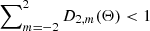 unless the star is aligned or totally misaligned. At Θ = 90°, where the reduction in the heating is the strongest, the increase in temperature is only ≳11% relative to the Θ = 0 or 180° cases. Despite the modified temperature evolution, the ratio between Tvis(t) and Tvis(t = −20) is the same as aligned systems. The weakened f-mode excitation may also change the inspiral trajectory, and thus the time before merger tp cannot be trivially compared from case to case. However, this effect results in at most 5 radians of de-phasing in the gravitational waveform for ν⋆ ≲ 100 Hz (Kuan & Kokkotas 2022), causing a ≪1 s error in the merger time prediction, so we ignore such complications here.
3. Spin frequency determination from precursor doubles
In this article, we assume that both precursors are set off from one star – either the primary (the one that forms earlier; see Sect. 2.2) or the companion – and further that they are attributable to g1 and g2 resonances. There are other theoretical possibilities, however, notably that non-g modes are responsible or that each star releases a flare at different times rather than one star releasing both. These are discussed in detail in Sect. 4.3.
The orbital frequencies at which two precursors, A and B, are observed, denoted by νA and νB with νA > νB, should be determined by their preceding time relative to the merger, while the measured quantity is the waiting time (i.e. the preceding time relative to the main burst). Therefore, νA and νB depend on the unknown jet formation timescale τjet for the associated SGRB when the waiting time are given. In addition, a resonant overstraining will not instantaneously lead to a precursor and there is some time delay between g-mode resonance and flare. In particular, there are two times to consider in a failure-induced flare scenario: (i) the time taken for the crust to fail following an overstraining from resonance, and (ii) the time for emissions to be generated following a failure (see also Thompson & Duncan 1995 for a discussion in the magnetar flare context). Tsang et al. (2012) estimate (i) to be ∼1 ms based on elastic-to-tidal energy ratios, though the value depends on both the overlap integral and mode frequency (see Eq. (10)). For (ii), Neill et al. (2022) argue that the timescale could be as long as ∼0.1 s for B ∼ 1013 G; see their Eq. (12). However, this estimate assumes σmax ∼ 0.1 estimated from Horowitz & Kadau (2009), though a more recent study by Baiko & Chugunov (2018) finds σmax ≈ 0.04. We estimate, following Neill et al. (2022),
 (22)
(22)
where Lmax is the rate at which energy can be extracted by the magnetic field. For even modestly bright precursors (cf. the precursor in GRB 211211A, with luminosity reaching ∼7 × 1049 erg s−1Xiao et al. 2022), temit is therefore sub-leading with respect to the observational uncertainties already present in estimating the precursor onset time (Coppin et al. 2020; Wang et al. 2020). (Note that we also ignore temperature changes to the lattice strain threshold, which reduces σmax, and thus temit is an overestimate for late-time precursors). In Table 2 below and throughout, we account for a ≳0.1 s tolerance in the onset time, absorbing uncertainties related to the two timescales described above.
In this work, the orbital evolution is numerically simulated by using a third-order post-Newtonian (PN) Hamiltonian, a 2.5 PN treatment for GW back-reaction, and the tidal effects of the l = 2 = mf modes (see Kuan et al. 2021b, for details). Following this notation, we denote the stratification indices at the time of the precursors as δA and δB. Matching the tidal-driving frequency to the inertial-frame frequencies of g1 and g2 modes gives us (from Eqs. (2) and (4))
 (23)
(23)
where m1 and m2 are the winding numbers associated with the g1 and g2 mode that accounts for the precursor, and the numerical coefficients come from the fitting parameter in Eq. (2) and the respective integrated constants C defined in (4).
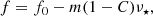
Although relation (23) holds for the EOS in Fig. 1, hereafter we limit ourselves to the EOSs able to support stars with masses ≳2 M⊙ or more so as to be consistent with Shapiro delay measurements of PSR J0740+6620 (Cromartie et al. 2020; Fonseca et al. 2021). These are listed in Fig. 5. This requirement for the maximal mass attainable of a certain EOS is conservative since we take the mass of this millisecond pulsar as a potential limit of static NSs, while J0740 spins at ∼346 Hz (see Table 1 of Cromartie et al. 2020). It is worth pointing out the recent discovery of PSR J0952-0607 may set a novel record on mass of NSs at M = 2.19 M⊙, which has a higher spin of ∼700 Hz nonetheless. In addition, we note that relation (23) does not depend on Θ, and acts as a necessary condition for double precursors but not a sufficient condition. The other conditions required within the resonance shattering scenario of g modes are: (i) the excitation occurring at the precursor timing should be strong enough to yield the crust, thus requiring a minimum magnitude to the tidal overlap3 and maximum on the inclination Θ, and (ii) the energy stored in the cracking area should be large enough to accommodate the luminosity of the precursor(s).
 |
Fig. 5. Derived spin of the primary (Eq. (24)) for double-precursor events with various EOSs in binaries with fixed total masses of 2.5 M⊙ and 2.8 M⊙ as functions of mass ratio q. Solid lines represent Eq. (25). |
We here do not take m ≤ 0 modes into account, as discussed in Sect. 2.4; accordingly, the axial quantum numbers of the modes for both precursors may take values of 1 and 2, leading to four possible combinations. As far as the inferred spin is concerned, the two extreme cases are, respectively, (m1, m2) = (1, 2) (smallest estimate) and (2, 1) (largest estimate). Although the difference can be larger than 100% (cf. Table 2), narrowing down the choice to only one or two can be, in principle, achieved when combining these data with other observations coming from, foe example, the kilonova (Papenfort et al. 2022), the presence or absence of spin-induced phase shifts in gravitational waveform (Steinhoff et al. 2021; Kuan & Kokkotas 2022), and from the nature of the accretion disc surrounding the merger site (East et al. 2019). In addition, the free-mode frequencies obtained retroactively from the spin estimate should be accessible (see below).
Spin predictions, in Hz, for a variety of different resonance scenarios (i.e. for different azimuth number combinations; last four columns) and relative precursors timings (tp; first column) in a GRB095010-like system with a tilted binary (i.e. Θ ≠ 0°; though note that the angle does not affect the inertial-frame mode frequency).
3.1. Case study: GRB 090510
GRB 090510 displayed two precursors at ∼13 s and ∼0.5 s prior to the main event (Abdo et al. 2009; Troja et al. 2010). Neglecting the jet formation timescale for now (i.e. taking τjet = 0 ms), we find νA = 68 − 80 Hz and νB = 22 − 25.5 Hz over a wide range of binaries for each of the considered EOSs: those with total mass Mtot = 2.5 − 3.1 M⊙ and mass ratios such that the lighter NS is heavier than 1 M⊙ (see below). With the complication introduced by the axial number discussed above in mind, we present results assuming m1 = 2 = m2 in this section, while discussion pertinent to other combinations is provided when appropriate. The m1 = m2 = 2 assumption is especially applicable to a star with an inclination Θ ≲ 40°, while it becomes less feasible if the star is strongly tilted (cf. Fig. 2).
Assuming δ = 0.005 at 20 s prior to merger, which is controlled by the compositional stratification mostly and suitable for a mature NS before a potential tidal heating (Xu & Lai 2017), the heating obtained via Eq. (20) gives the stratifications δA, B at the time of each precursor. An analysis over a uniform spread of stellar masses and radii, spanning 1 − 2.2 M⊙ and 10.5 − 13 km, and mass ratio over 0.7 − 1, reveals that the inferred values of δA, B are rather insensitive to these three parameters, with the strongest dependence being on M⋆. Over the whole parameter space, we find δA ≃ 0.021 and δB ≃ 0.006 with errors of only 10−4 for δA, and 10−7 for δB. We caution the reader that the narrow error bars on both δA and δB result from our simple heating model (Sect. 2.5), which may not approximate well the situation where crustal heating is treated rigorously as in, for example, van Riper et al. (1991) and Pan et al. (2020). The stratifications at the occurrences of the two precursors therefore do not depend on the aforementioned three quantities except in a mild way, implying that we can measure the spin of the NS hosting the double regardless of whether it is the primary or companion.
After fixing the respective values of δ, the denominator of Eq. (23) is found to be roughly constant: for the aforementioned prior of stellar parameters, the denominator4 has a normal distribution with a mean of 2.2099 and a standard deviation of 0.0128. This fact simplifies Eq. (23) to one solely in terms of the orbital frequencies as
![Mathematical equation: $$ \begin{aligned} \nu _\star (\nu _A,\nu _B,\tau _{\text{jet}}) \approx 0.45\times [1.24\nu _A(\tau _{\text{jet}})-3.74\nu _B(\tau _{\text{jet}})+\beta ]. \end{aligned} $$](/articles/aa/full_html/2023/08/aa46658-23/aa46658-23-eq30.gif) (24)
(24)
The spin for the combination m1 = 2 = m2 is, therefore, well approximated as a function of the chirp mass ℳ alone, in the form
 (25)
(25)
The above holds because the orbital evolution is to a large measure determined by ℳ, even though tidal forces and the stellar f modes influence orbital dynamics; this is also the main reason why, in GW analysis, ℳ can be measured rather accurately. For a ‘canonical’ case with ν⋆ = 3.28 Hz, the free-mode frequencies of the g1 and g2 modes are found to be, respectively, ∼145 − 165 Hz for δ = δA and ∼50 − 57 Hz for δ = δB depending on M⋆ and the EOS. An important aspect to note is that an MPA1 NS, having frequencies in the aforementioned ranges for the g1 and g2 modes, is close to the range of tidal-neutral models. In this sense, this EOS may be in tension with this scenario for the double precursors with timing similar to the two of GRB090510.
Although we focus on the combination of m1 = 2 = m2 here, the variation in the inferred spin due to different combinations is explored in Table 2, where we summarise the predicted spin of an APR4 NS having 1.4 M⊙ in a binary with q = 1 for GRB090510 under all possible combinations, including possible errors on the precursor timing. We see that for a given timing of the double precursors (i.e. the same row in Table 2), the spin can have four possible values, which vary by over 100%. In addition, an uncertainty of 0.1 s in the timing of the later (i.e. smaller tp) precursor can lead to an error of ≳10 Hz in the spin estimate as shown in the first three rows of Table 2. The reason behind this susceptibility is that the orbital frequency changes rapidly in the last stages before merger; in particular, an uncertainty of ∼0.1 s between tp = 0.45 and tp = 0.55 corresponds to a increase of ≳5 Hz in the orbital frequency (see Sect. 3.2 for more detail). Similar changes in the predicted spin are observed if the earlier precursor has a timing error of ≳1 s.
Taking two specific binary sequences, each characterised by a fixed total mass, we plot ν⋆ in Fig. 5 as a function of the mass ratio, q, where the solid lines represent the respective fittings (25). We see that ν⋆ depends only weakly on both q (differs by less than 1 Hz between q = 1 and q = 0.75) and the EOS. For Mtot = 2.5 M⊙, one may expect the remnant to be supra-massive or even stable for the MPA1 EOS (stiffest one studied), surviving collapse long enough to produce an X-ray afterglow (see Sect. 4.2), as appropriate for GRB 090510. For this total mass, we do not consider values q < 0.75 since q ≈ 0.75 implies a very light companion with ∼1.07 M⊙; this would be in tension with the lightest known NS, viz. the secondary of J0453+1559 (1.18 M⊙; Martinez et al. 2015). By contrast, a hyper-massive remnant may be expected for Mtot ≳ 2.8 M⊙. It is worth mentioning that the lighter NS for the considered supra-massive remnant cases is more susceptible to the tidal push since g modes in NSs with mass closer to 1.45 M⊙ are more tidally neutral (see Appendix A of Kuan et al. 2022).
Although the inference of spin is largely insensitive to q, the extent to which a mode can be excited depends on q. These factors, together with Θ, M⋆, q, and EOS, are core to the rather involved problem of whether the generated strain is strong enough (which also depends on the crust model; see Baiko & Chugunov 2018). Since the present article aims to point out the necessary condition (23), we defer this complicated, multi-dimensional issue to a future study.
3.2. Jet delay corrections
Allowing for a non-zero jet formation and breakout timescale, τjet, gives rise to a shift δν⋆ in the spin inference from Eq. (25). Since the binary evolution is largely determined by ℳ, it is expected that the mode frequencies associated with a given precursor timing is a function of ℳ to the leading order. That said, νA and νB in Eq. (23) can be estimated accurately if ℳ is given, while the stratifications relevant to the tidal heating are subject to the influence of the mass ratio, as suggested in Eq. (20). However, for a fixed ℳ, the dependence of Tvis, a on q is only slight. In particular, the dependence on q is encoded in the combination  , which is rather insensitive to q as shown in Fig. 6. While in Fig. 6 we only show the results for EOS MPA1, we note that the dependence on q is weak for all the considered EOSs. For example, the heating difference in the heavier (or equally heavy) star between q = 1 and q = 0.7 cases is only ∼2.5%. The weak influence of q on the ratio
  is at a roughly the same level since δ ∝ T2. In addition, this deviation is independent of ℳ. Accordingly, Eq. (24) is modified as
![Mathematical equation: $$ \begin{aligned}&\nu _\star (\nu _A,\nu _B,\tau _{\text{jet}}) \approx 0.45\times \Big [ 1.24\nu _A(\tau _{\text{jet}})\nonumber \\&\qquad \qquad \qquad -(3.65\pm 0.09)\nu _B(\tau _{\text{jet}})+\beta \Big ] \end{aligned} $$](/articles/aa/full_html/2023/08/aa46658-23/aa46658-23-eq34.gif) (26)
(26)
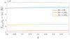 |
Fig. 6. Compactness-scaled Tvis, a, as a function of q, for three representative chirp masses, ℳ. The MPA1 EOS is used to obtain R⋆ from the stellar mass, M⋆, derived from ℳ and q. |
to engulf the uncertainty of q in the range of 0.7 ≤ q ≤ 1.
For τjet ≲ 200 ms (Zhang 2019), and for the specific situation detailed in Sect. 3.1, we find the relation weakly depends on ℳ:
![Mathematical equation: $$ \begin{aligned}&\delta \nu _\star /\nu _\star \approx (0.83\pm 0.13)\left(\frac{\tau _{\text{jet}}}{100\mathrm{ms}}\right) +(0.20\pm 0.03)\left(\frac{\tau _{\text{jet}}}{100\mathrm{ms}}\right)^2 \nonumber \\&-\left[(0.11\pm 0.03)\left(\frac{\tau _{\text{jet}}}{100\mathrm{ms}}\right) +(0.03\pm 0.01)\left(\frac{\tau _{\text{jet}}}{100\mathrm{ms}}\right)^2\right]\frac{\mathcal{M}}{M_{\odot }}, \end{aligned} $$](/articles/aa/full_html/2023/08/aa46658-23/aa46658-23-eq35.gif) (27)
(27)
where the error budgets in coefficients are due to the uncertainty of precursor timing. If the SGRB takes less than 20 ms to launch and break out, for instance, the correction is ≲15% while the exact value depends on ℳ and q.
4. Connections to other observational channels
In this section we explore some connections that the double precursor scenario has to GWs (Sect. 4.1) and X-rays afterglow (Sect. 4.2), and also provide some discussion about how non-g-mode scenarios can still be used to constrain the stellar properties (Sect. 4.3).
4.1. Gravitational waves
There are two phases for which GW measurements can augment our knowledge about systems with precursors: during the merger and from the remnant. During merger, tidal resonances, and forces more generally, accelerate the inspiral. These influences on the waveform may be connected back properties of the pre-merger stars to infer not only ℳ, q, and the effective spin parameter of binaries χeff (Zhu & Ashton 2020) but also the stellar compactnesses via the mutual deformability,  . Generally speaking however,
  can only be tightly constrained by using priors for ν⋆ (Abbott et al. 2017; Annala et al. 2018) since (i) the spins also induce certain de-phasing in the gravitational waveform, degenerate with that caused by tidal activities, and (ii) the spin-modulated QNM spectrum may enhance the tidal contribution in the de-phasing (Steinhoff et al. 2021; Kuan & Kokkotas 2022). From the waveform (de)phasing, it is also possible to constrain the influence of unstable couplings between p and g modes (Abbott et al. 2019a; Reyes & Brown 2020), where the amplitude is collectively set a collection of excited p–g pairs (Weinberg et al. 2013; Essick et al. 2016).
In addition, gravitational radiation from the remnant, which may be observed either directly or via the fall-off slope of electromagnetic emissions (see Sect. 4.2; Lasky & Glampedakis 2016), allow us to infer properties of the final star. It was shown by Manoharan et al. (2021) that many stellar parameters, such as the compactness, of a long-lived remnant NS (i.e. when Mtot ≲ 2.5 M⊙; see Fig. 5) can also be inferred from the mutual tidal deformability. Furthermore, the mass of the remnant may be reliably estimated from the chirp mass to within an error of at most ≲0.1 M⊙ (Bauswein et al. 2016). The frequency of the f mode, from which independent constraints on the EOS can be placed, in the remnant can also be predicted if the spin frequency is known (Krüger & Kokkotas 2020). Additionally, large pre-merger spins may result in high degrees of mass asymmetry in the remnant (Papenfort et al. 2022), possibly revealing itself through the so-called one-arm instability in the GW spectrum or shifting the bar-mode peak (East et al. 2019). Under favourable orientations, (unstable) QNMs from the rapidly spinning remnant may be observable with the Einstein Telescope out to ≳200 Mpc (Doneva et al. 2015).
4.2. Afterglow light curves
GRB 090510 (and many other SGRBs) displayed an afterglow ‘plateau’, which suggests that a NS was born following the merger (Ciolfi 2020). Depending on the compactness and spin-down radiation efficiency of the remnant, analyses of the light curve indicate that the newborn star had a period in the range 1.8 − 8 ms, surface magnetic field strength of (5 − 17)×1015 G, and quadrupolar ellipticity between 10−4 and 10−2 (Rowlinson et al. 2013; Suvorov & Kokkotas 2020a, 2021). These features impact the potential GW signal; for example, the characteristic strain  . From a purely electromagnetic standpoint, an eventual fall-off slope of −2 in the X-ray emissions would be expected for dipolar spin down, while GW-dominated energy losses would be characterised by a slope of −1 instead, the crossover time and luminosity of which can be used to infer the ellipticity and (surface) magnetic field strength (Lasky & Glampedakis 2016). As the spin of the pre-merger stars has an impact on the properties of the remnant (Kastaun et al. 2017; East et al. 2019; Papenfort et al. 2022), information gleaned from double precursors may reduce the error bars from afterglow analysis. It is worth pointing out that a merger that leaves behind a stable NS, rather than a black hole or hyper-massive remnant (cf. Fig. 5), must be composed of relatively light stars, likely having formed through ‘bare collapse’ or electron capture supernovae (Podsiadlowski et al. 2004).
4.3. Other scenarios leading to double precursors
Although we focus on g-mode scenarios in this work, it is worth briefly commenting on other possibilities, and what one may infer under those circumstances. Indeed, precursors can arise from three different factors. The first is resonances from other modes, such as i or s modes (Tsang et al. 2012; Tsang 2013), ocean modes in low metallicity crusts (Sullivan et al. 2023), or even f or r modes in rapidly rotating or ultra-magnetised systems (Suvorov & Kokkotas 2020b).
The second is each star undergoing a separate fracture, rather than one star undergoing two. Different atomic impurities in the crust, for example, could imply that the von Mises (or some other) criterion is met at different strains and frequencies in each star. Such a scenario would be favoured if, for example, the stellar crust cannot ‘heal’ in between fractures; see Schneider et al. (2018), Kerin & Melatos (2022) and references therein.
The third involves scenarios unrelated to modes, such as the unipolar inductor model, where electromotive forces, generated across a weakly magnetised star as it moves through the magnetosphere of a magnetar companion, spark precursor emissions (Piro 2012; Lai 2012).
It is beyond the scope of this work to go into detail about each of these possibilities, though we explore the first point here. In an agnostic analysis, the two precursors of GRB 090510 corresponds to two l = 2 = m modes (see Sect. 2.1) with inertial-frame frequencies of ∼160 Hz and ∼50 Hz, respectively, assuming an aligned system (cf. Sect. 2.4). Given the large difference in the frequencies of i and s modes (see e.g., Fig. 3 in Passamonti & Andersson 2012), it seems difficult to connect both of these crust-induced modes to the two precursors of GRB090510. In particular, even though the earlier flare may be accommodated by an i mode for an almost-static star, it is difficult to accommodate the later flare with i modes (Tsang et al. 2012; Passamonti et al. 2021). However, we note that it could be possible to account for these two pre-emissions with a mix of i and s modes, which calls for an s mode with free-mode frequency ∼160 Hz since, for an i mode to cause first precursor, we must have ν⋆ ≪ 10 Hz. This mixed-mode scenario will be investigated thoroughly elsewhere.
Some stars in coalescing binaries may spin rapidly, for example the secondary of GW190814 (Biswas et al. 2021), where modes with high free frequencies (e.g., f modes) become of interest (Suvorov & Kokkotas 2020b). Nonetheless, if such high spins align with the orbit, we should see a rotation-induced modulation in the light curves during the sub-second timescale of the observed precursors (Stachie et al. 2022). Unless the spin is misaligned with the orbit, the absence of substructure hints that ν⋆ ≲ 100 Hz for precursor hosts.
5. Discussion and summary
A system that displays a double precursor, is bright and/or near enough (≲100 Mpc with aLIGO) to be detected in GWs at the time of the merger and late inspiral, and shows an X-ray plateau post-GRB might be something of a holy grail for high-energy astrophysics. As shown here, the first two of these observation bundles allow for the mass, radius, and spin of (at least one of) the pre-merger stars to be determined with high accuracy. In principle, this can then be connected to the properties of the post-merger remnant by combining numerical, merger simulations (Kastaun et al. 2017; East et al. 2019; Papenfort et al. 2022) with the spin-down luminosity inferred from the jet energetics (Ciolfi 2020) and X-ray plateau (Rowlinson et al. 2013). One may therefore be able to establish a magnetic field strength, compactness, and spin for the remnant (Suvorov & Kokkotas 2020a, 2021; Manoharan et al. 2021), which imply constraints on the nuclear EOS (e.g., Biswas et al. 2021). If the unstable part of the QNM spectrum of the rapidly spinning remnant is also observable (out to ≳200 Mpc with the Einstein Telescope; Doneva et al. 2015), the error bars may shrink significantly.
Binary NSs tend to spin slowly; the fastest known binary pulsar is J0737-3039A, with a spin frequency of 44 Hz (Burgay et al. 2003). For GRB 090510 we predict that the star emitting the two precursors has ν⋆ ≈ 3 Hz if l = 2 = mg1- and g2-mode resonances spark the precursors (Table 2), which is lower than this value. We note that the spin estimate given above is insensitive to both the EOS (modulo the caveats mentioned in Sect. 2.1) and q (Fig. 5). On the other hand, if the associated modes have different combinations of quantum numbers because of a significant tilt, Θ ≳ 30° (on par with the greatest limit set on PSR J1756-2251, ≤34°, as inferred from geodetic precession; Ferdman et al. 2014), the inferred spin ranges from 2 ≲ ν⋆/Hz ≲ 13 assuming an instantaneous jet breakout and perfect precision on the timing measurements. In reality, the uncertainty is more likely to cover the range 2 ≲ ν⋆/Hz ≲ 20 if we remain agnostic regarding these factors (see Table 2 and Sect. 3.2). This is especially true because of our simplified prescription for introducing the adiabatic index of the perturbed star (see the caveats noted in Sect. 2.1 and elsewhere). Despite the uncertainty in the quantum numbers, we only have four possibilities for the spin, any of which can serve as a necessary condition when accounting for double precursors via g1 and g2 modes (see the discussion in Sect. 3), and the method demonstrates, in principle, how additional information can be extracted from doubles.
In addition to frequency matching, the modes must be excited strongly enough to shatter the crust. The extent to which a mode can be amplified by the tidal field depends on the mass of the other star, the inclination of the spin, and the tidal overlap of the mode. In other words, an observation of two precursors can place certain constraints on the range of the aforementioned quantities. For example, a star with mass 1.45 M⊙ may not be able to yield its crust via g-mode resonances due to the tidal neutrality of these modes (Kuan et al. 2022). In addition, non-zero inclinations will weaken the mode excitations in general (not just g modes); thus, the observation of resonant-shattering flares can set a limit on the tilt angle of erupting NSs. Together with the inferred spin, such a study may shed light on the binary formation channel; for example, a NS member spinning at a low rate with a small tilt angle could rule out a scenario where the primary is long-term recycled and aligned (see Sect. 2.3 for further discussion).
Although only one double precursor event (in a SGRB) has thus far been observed, in the future one may be able to – assuming a resonance scenario – place statistical constraints on the spin dynamics of NS binaries that do not exhibit pulsations. This would allow for an investigation of the evolutionary pathways of NSs that reside within the so-called pulsar graveyard. It is also conceivable that even millisecond objects enter into compact binaries in dense astrophysical environments through dynamical exchanges. This raises the question as to what the timing data of double precursors would look like in such a case. According to Eq. (23), for spin frequencies ν⋆ ≫ 10 Hz, the two events should be separated by at least 15 s, a prediction that is robust for different EOSs. Depending on the spin alignment of the binary constituents, large values of ν⋆ may excite the so-called one-arm instability in the GW spectrum of the remnant and enhance blue and/or red kilonovae (East et al. 2019; Papenfort et al. 2022).
We close by noting that magnetic fields have not been considered at all in this work. It is likely that magnetic fields play a significant role in extracting the elastic energy from the crust that eventually fuels the precursor (Tsang 2013; Suvorov & Kokkotas 2020b; Suvorov et al. 2022). However, unless the fields are of magnetar-level strength (B⋆ ≳ 1015 G), the Lorentz force will not be strong enough to significantly distort the QNM spectrum (Kuan et al. 2021a), implying that the spin-fitting formula (23) would remain unchanged. Even so, Suvorov & Kokkotas (2020b) argue that precursors with non-thermal spectra may be indicative of intense magnetic fields, which would prevent thermalisation from pair-photon cascades created via mode-induced back-reactions (see also Tsang et al. 2012; Zhong et al. 2019; Kuan et al. 2021b). These considerations therefore imply that the error bars presented for the spin-frequency measurements may be slightly underestimated, at least when applied to double precursors that show predominantly non-thermal spectra (as was the case for GRB090510; Troja et al. 2010).
Using the introduced stratification parameterisation we find, for a family of WFF EOSs, the g1-mode frequency is ∼90 Hz for a NS with M⋆ = 1.4 M⊙ and δ = 0.005. This matches the self-consistently obtained frequencies of Lai (1994) to within 20% (e.g., for the EOS we call WFF1 but they call ‘AU’, we find 93.03 (61.11) Hz while they get 72.6 (51.4) Hz for the g1- (g2-)mode frequency). Note also that Lai (1994) uses a Newtonian scheme while ours is general-relativistic, likely accounting for most of the disparity. The validity of the spatially constant δ approximation specifically is detailed in Appendix A.
This expression differs slightly from Eq. (10) in Kuan et al. (2022) due to a typographical error in that work. Nonetheless, the results therein are essentially unaffected: g-spectra with spatially varying δ were in fact computed in Kuan et al. (2022), where it was concluded that (i) the g-spectrum is largely determined by the surface temperature since only in the outer most part of the star can buoyancy be comparable to the isotropic pressure, and (ii) the constant δ approximation works well for surface temperatures below ∼1010 K.
It has been shown in the Appendix of Kuan et al. (2022) that the g modes of stars with mass close to 1.45 M⊙ are less susceptible to the tidal field, and thus are less likely to break the crust.
The mean for combinations (m1, m2) = {(1, 2), (2, 1), (1, 1)} is collectively listed as {2.7629, 0.5519, 1.1049} with respective standard deviations of {0.0129, 0.0068, 0.0064}. These values can be substituted in the denominator of Eq. (23) to get the formula similar to Eq. (24) suitable for the associated combination of (m1, m2).
Acknowledgments
KK gratefully acknowledges financial support by DFG research Grant No. 413873357. HJK recognises support from Sandwich grant (JYP) No. 109-2927-I- 007-503 by DAAD and MOST during early stages of this work. AGS is grateful for funding received from the European Union’s Horizon 2020 Programme under the AHEAD2020 project (grant n. 871158) and the Alexander von Humboldt foundation. We thank the anonymous referee for their helpful feedback.
References
- Abbott, B. P., Abbott, R., Abbott, T. D., LIGO Scientific Collaboration& Virgo Collaboration 2017, Phys. Rev. Lett., 119, 161101 [Google Scholar]
- Abbott, B. P., Abbott, R., Abbott, T. D., et al. 2019a, Phys. Rev. Lett., 122, 061104 [NASA ADS] [CrossRef] [Google Scholar]
- Abbott, B. P., Abbott, R., Abbott, T. D., et al. 2019b, Phys. Rev. X, 9, 011001 [Google Scholar]
- Abbott, B. P., Abbott, R., Abbott, T. D., The LIGO Scientific Collaboration& Virgo Collaboration 2020, CQG, 37, 045006 [NASA ADS] [CrossRef] [Google Scholar]
- Abdo, A. A., Ackermann, M., Ajello, M., et al. 2009, Nature, 462, 331 [NASA ADS] [CrossRef] [Google Scholar]
- Akgün, T., Reisenegger, A., Mastrano, A., & Marchant, P. 2013, MNRAS, 433, 2445 [Google Scholar]
- Andersson, N., & Kokkotas, K. D. 1998, MNRAS, 299, 1059 [NASA ADS] [CrossRef] [Google Scholar]
- Annala, E., Gorda, T., Kurkela, A., & Vuorinen, A. 2018, Phys. Rev. Lett., 120, 172703 [Google Scholar]
- Baiko, D. A., & Chugunov, A. I. 2018, MNRAS, 480, 5511 [NASA ADS] [CrossRef] [Google Scholar]
- Bauswein, A., Stergioulas, N., & Janka, H.-T. 2016, Eur. Phys. J. A, 52, 56 [NASA ADS] [CrossRef] [Google Scholar]
- Beloborodov, A. M., & Li, X. 2016, ApJ, 833, 261 [NASA ADS] [CrossRef] [Google Scholar]
- Biswas, B., Nandi, R., Char, P., Bose, S., & Stergioulas, N. 2021, MNRAS, 505, 1600 [NASA ADS] [CrossRef] [Google Scholar]
- Burgay, M., D’Amico, N., Possenti, A., et al. 2003, Nature, 426, 531 [NASA ADS] [CrossRef] [Google Scholar]
- Chamel, N., & Haensel, P. 2006, Phys. Rev. C, 73, 045802 [NASA ADS] [CrossRef] [Google Scholar]
- Ciolfi, R. 2020, Gen. Rel. Grav., 52, 59 [NASA ADS] [CrossRef] [Google Scholar]
- Coppin, P., de Vries, K. D., & van Eijndhoven, N. 2020, Phys. Rev. D, 102, 103014 [Google Scholar]
- Cromartie, H. T., Fonseca, E., Ransom, S. M., et al. 2020, Nat. Astron., 4, 72 [NASA ADS] [CrossRef] [Google Scholar]
- Doneva, D. D., Kokkotas, K. D., & Pnigouras, P. 2015, Phys. Rev. D, 92, 104040 [NASA ADS] [CrossRef] [Google Scholar]
- Doroshenko, V., Poutanen, J., Tsygankov, S. S., et al. 2022, Nat. Astron., 6, 1433 [NASA ADS] [CrossRef] [Google Scholar]
- Duncan, R. C. 1998, ApJ, 498, L45 [NASA ADS] [CrossRef] [Google Scholar]
- East, W. E., Paschalidis, V., Pretorius, F., & Tsokaros, A. 2019, Phys. Rev. D, 100, 124042 [NASA ADS] [CrossRef] [Google Scholar]
- Essick, R., Vitale, S., & Weinberg, N. N. 2016, Phys. Rev. D, 94, 103012 [NASA ADS] [CrossRef] [Google Scholar]
- Ferdman, R. D., Stairs, I. H., Kramer, M., et al. 2013, ApJ, 767, 85 [NASA ADS] [CrossRef] [Google Scholar]
- Ferdman, R. D., Stairs, I. H., Kramer, M., et al. 2014, MNRAS, 443, 2183 [NASA ADS] [CrossRef] [Google Scholar]
- Fonseca, E., Stairs, I. H., & Thorsett, S. E. 2014, ApJ, 787, 82 [NASA ADS] [CrossRef] [Google Scholar]
- Fonseca, E., Cromartie, H. T., Pennucci, T. T., et al. 2021, ApJ, 915, L12 [NASA ADS] [CrossRef] [Google Scholar]
- Fujibayashi, S., Kiuchi, K., Nishimura, N., Sekiguchi, Y., & Shibata, M. 2018, ApJ, 860, 64 [NASA ADS] [CrossRef] [Google Scholar]
- Gaertig, E., & Kokkotas, K. D. 2009, Phys. Rev. D, 80, 064026 [NASA ADS] [CrossRef] [Google Scholar]
- Gao, H., Lei, W.-H., & Zhu, Z.-P. 2022, ApJ, 934, L12 [NASA ADS] [CrossRef] [Google Scholar]
- Glampedakis, K., & Suvorov, A. G. 2021, MNRAS, 508, 2399 [CrossRef] [Google Scholar]
- Gourgouliatos, K. N., & Cumming, A. 2014, Phys. Rev. Lett., 112, 171101 [NASA ADS] [CrossRef] [Google Scholar]
- Gudmundsson, E. H., Pethick, C. J., & Epstein, R. I. 1982, ApJ, 259, L19 [CrossRef] [Google Scholar]
- Gupta, P. K., Steinhoff, J., & Hinderer, T. 2023, ArXiv e-prints [arXiv:2302.11274] [Google Scholar]
- Haensel, P., Levenfish, K. P., & Yakovlev, D. G. 2002, A&A, 394, 213 [NASA ADS] [CrossRef] [EDP Sciences] [Google Scholar]
- Horowitz, C. J., & Kadau, K. 2009, Phys. Rev. Lett., 102, 191102 [NASA ADS] [CrossRef] [Google Scholar]
- Jaikumar, P., Semposki, A., Prakash, M., & Constantinou, C. 2021, Phys. Rev. D, 103, 123009 [NASA ADS] [CrossRef] [Google Scholar]
- Kanakis-Pegios, A., Koliogiannis, P. S., & Moustakidis, C. C. 2022, Phys. Lett. B, 832, 137267 [NASA ADS] [CrossRef] [Google Scholar]
- Kastaun, W., Ciolfi, R., Endrizzi, A., & Giacomazzo, B. 2017, Phys. Rev. D, 96, 043019 [NASA ADS] [CrossRef] [Google Scholar]
- Kerin, A. D., & Melatos, A. 2022, MNRAS, 514, 1628 [CrossRef] [Google Scholar]
- Kokkotas, K. D., & Schafer, G. 1995, MNRAS, 275, 301 [NASA ADS] [CrossRef] [Google Scholar]
- Kramer, M. 1998, ApJ, 509, 856 [NASA ADS] [CrossRef] [Google Scholar]
- Krüger, C. J., & Kokkotas, K. D. 2020, Phys. Rev. Lett., 125, 111106 [CrossRef] [Google Scholar]
- Krüger, C. J., Ho, W. C. G., & Andersson, N. 2015, Phys. Rev. D, 92, 063009 [CrossRef] [Google Scholar]
- Kuan, H.-J., & Kokkotas, K. D. 2022, Phys. Rev. D, 106, 064052 [NASA ADS] [CrossRef] [Google Scholar]
- Kuan, H.-J., Suvorov, A. G., & Kokkotas, K. D. 2021a, MNRAS, 508, 1732 [NASA ADS] [CrossRef] [Google Scholar]
- Kuan, H.-J., Suvorov, A. G., & Kokkotas, K. D. 2021b, MNRAS, 506, 2985 [NASA ADS] [CrossRef] [Google Scholar]
- Kuan, H.-J., Krüger, C. J., Suvorov, A. G., & Kokkotas, K. D. 2022, MNRAS, 513, 4045 [NASA ADS] [CrossRef] [Google Scholar]
- Lai, D. 1994, MNRAS, 270, 611 [NASA ADS] [CrossRef] [Google Scholar]
- Lai, D. 2012, ApJ, 757, L3 [NASA ADS] [CrossRef] [Google Scholar]
- Lai, D., & Wu, Y. 2006, Phys. Rev. D, 74, 024007 [NASA ADS] [CrossRef] [Google Scholar]
- Lasky, P. D., & Glampedakis, K. 2016, MNRAS, 458, 1660 [NASA ADS] [CrossRef] [Google Scholar]
- Lattimer, J. M. 2012, Ann. Rev. Nucl. Part. Sci., 62, 485 [NASA ADS] [CrossRef] [Google Scholar]
- Link, B., & Epstein, R. I. 1996, ApJ, 457, 844 [NASA ADS] [CrossRef] [Google Scholar]
- Ma, S., Yu, H., & Chen, Y. 2021, Phys. Rev. D, 103, 063020 [NASA ADS] [CrossRef] [Google Scholar]
- Manoharan, P., Krüger, C. J., & Kokkotas, K. D. 2021, Phys. Rev. D, 104, 023005 [NASA ADS] [CrossRef] [Google Scholar]
- Martinez, J. G., Stovall, K., Freire, P. C. C., et al. 2015, ApJ, 812, 143 [NASA ADS] [CrossRef] [Google Scholar]
- Miao, Z., Zhou, E., & Li, A. 2023, ArXiv e-prints [arXiv:2305.08401] [Google Scholar]
- Minaev, P., Pozanenko, A., & Molkov, S. 2018, Int. J. Mod. Phys. D, 27, 1844013 [NASA ADS] [CrossRef] [Google Scholar]
- Neill, D., Tsang, D., van Eerten, H., Ryan, G., & Newton, W. G. 2022, MNRAS, 514, 5385 [NASA ADS] [CrossRef] [Google Scholar]
- Oertel, M., Hempel, M., Klähn, T., & Typel, S. 2017, Rev. Mod. Phys., 89, 015007 [Google Scholar]
- Paczyński, B. 1971, ARA&A, 9, 183 [Google Scholar]
- Pan, Z., Lyu, Z., Bonga, B., Ortiz, N., & Yang, H. 2020, Phys. Rev. Lett., 125, 201102 [CrossRef] [Google Scholar]
- Papenfort, L. J., Most, E. R., Tootle, S., & Rezzolla, L. 2022, MNRAS, 513, 3646 [CrossRef] [Google Scholar]
- Passamonti, A., & Andersson, N. 2012, MNRAS, 419, 638 [NASA ADS] [CrossRef] [Google Scholar]
- Passamonti, A., Haskell, B., Andersson, N., Jones, D. I., & Hawke, I. 2009, MNRAS, 394, 730 [NASA ADS] [CrossRef] [Google Scholar]
- Passamonti, A., Andersson, N., & Pnigouras, P. 2021, MNRAS, 504, 1273 [NASA ADS] [CrossRef] [Google Scholar]
- Piro, A. L. 2012, ApJ, 755, 80 [NASA ADS] [CrossRef] [Google Scholar]
- Podsiadlowski, P., Langer, N., Poelarends, A. J. T., et al. 2004, ApJ, 612, 1044 [NASA ADS] [CrossRef] [Google Scholar]
- Postnov, K. A., & Yungelson, L. R. 2014, Liv. Rev. Rel., 17, 3 [NASA ADS] [CrossRef] [Google Scholar]
- Potekhin, A. Y., Chabrier, G., & Yakovlev, D. G. 1997, A&A, 323, 415 [NASA ADS] [Google Scholar]
- Reisenegger, A. 2001, ApJ, 550, 860 [NASA ADS] [CrossRef] [Google Scholar]
- Reisenegger, A. 2009, A&A, 499, 557 [NASA ADS] [CrossRef] [EDP Sciences] [Google Scholar]
- Reyes, S., & Brown, D. A. 2020, ApJ, 894, 41 [NASA ADS] [CrossRef] [Google Scholar]
- Rowlinson, A., O’Brien, P. T., Metzger, B. D., Tanvir, N. R., & Levan, A. J. 2013, MNRAS, 430, 1061 [NASA ADS] [CrossRef] [Google Scholar]
- Schneider, A. S., Caplan, M. E., Berry, D. K., & Horowitz, C. J. 2018, Phys. Rev. C, 98, 055801 [NASA ADS] [CrossRef] [Google Scholar]
- Stachie, C., Dal Canton, T., Christensen, N., et al. 2022, ApJ, 930, 45 [CrossRef] [Google Scholar]
- Steinhoff, J., Hinderer, T., Buonanno, A., & Taracchini, A. 2016, Phys. Rev. D, 94, 104028 [NASA ADS] [CrossRef] [Google Scholar]
- Steinhoff, J., Hinderer, T., Dietrich, T., & Foucart, F. 2021, Phys. Rev. Res., 3, 033129 [NASA ADS] [CrossRef] [Google Scholar]
- Sullivan, A. G., Alves, L. M. B., Spence, G. O., et al. 2023, MNRAS, 520, 6173 [NASA ADS] [CrossRef] [Google Scholar]
- Suvorov, A. G., & Kokkotas, K. D. 2020a, Phys. Rev. D, 101, 083002 [NASA ADS] [CrossRef] [Google Scholar]
- Suvorov, A. G., & Kokkotas, K. D. 2020b, ApJ, 892, L34 [NASA ADS] [CrossRef] [Google Scholar]
- Suvorov, A. G., & Kokkotas, K. D. 2021, MNRAS, 502, 2482 [NASA ADS] [CrossRef] [Google Scholar]
- Suvorov, A. G., & Melatos, A. 2020, MNRAS, 499, 3243 [NASA ADS] [CrossRef] [Google Scholar]
- Suvorov, A. G., Mastrano, A., & Geppert, U. 2016, MNRAS, 459, 3407 [NASA ADS] [CrossRef] [Google Scholar]
- Suvorov, A. G., Kuan, H. J., & Kokkotas, K. D. 2022, A&A, 664, A177 [NASA ADS] [CrossRef] [EDP Sciences] [Google Scholar]
- Tauris, T. M., Langer, N., & Podsiadlowski, P. 2015, MNRAS, 451, 2123 [NASA ADS] [CrossRef] [Google Scholar]
- Tauris, T. M., Kramer, M., Freire, P. C. C., et al. 2017, ApJ, 846, 170 [Google Scholar]
- Thompson, C., & Duncan, R. C. 1995, MNRAS, 275, 255 [Google Scholar]
- Troja, E., Rosswog, S., & Gehrels, N. 2010, ApJ, 723, 1711 [NASA ADS] [CrossRef] [Google Scholar]
- Tsang, D. 2013, ApJ, 777, 103 [NASA ADS] [CrossRef] [Google Scholar]
- Tsang, D., Read, J. S., Hinderer, T., Piro, A. L., & Bondarescu, R. 2012, Phys. Rev. Lett., 108, 011102 [NASA ADS] [CrossRef] [Google Scholar]
- Typel, S., Oertel, M., & Klähn, T. 2015, Phys. Part. Nucl., 46, 633 [CrossRef] [Google Scholar]
- Typel, S., Oertel, M., Klähn, T., et al. 2022, ArXiv e-prints [arXiv:2203.03209] [Google Scholar]
- Unno, W., Osaki, Y., Ando, H., Saio, H., & Shibahashi, H. 1989, Nonradial Oscillations of Stars (Tokyo: University of Tokyo Press) [Google Scholar]
- van den Heuvel, E. P. J. 2017, J. Astrophys. Astron., 38, 45 [NASA ADS] [CrossRef] [Google Scholar]
- van Riper, K. A., Epstein, R. I., & Miller, G. S. 1991, ApJ, 381, L47 [NASA ADS] [CrossRef] [Google Scholar]
- Vavoulidis, M., Kokkotas, K. D., & Stavridis, A. 2008, MNRAS, 384, 1711 [NASA ADS] [CrossRef] [Google Scholar]
- Wang, J.-S., Peng, Z.-K., Zou, J.-H., Zhang, B.-B., & Zhang, B. 2020, ApJ, 902, L42 [NASA ADS] [CrossRef] [Google Scholar]
- Weinberg, N. N., Arras, P., & Burkart, J. 2013, ApJ, 769, 121 [NASA ADS] [CrossRef] [Google Scholar]
- Xiao, S., Zhang, Y. Q., Zhu, Z. P., et al. 2022, ArXiv e-prints [arXiv:2205.02186] [Google Scholar]
- Xu, W., & Lai, D. 2017, Phys. Rev. D, 96, 083005 [NASA ADS] [CrossRef] [Google Scholar]
- Yu, H., & Weinberg, N. N. 2017, MNRAS, 464, 2622 [NASA ADS] [CrossRef] [Google Scholar]
- Yu, H., Weinberg, N. N., Arras, P., Kwon, J., & Venumadhav, T. 2023, MNRAS, 519, 4325 [NASA ADS] [CrossRef] [Google Scholar]
- Zahn, J. P. 1977, A&A, 500, 121 [NASA ADS] [Google Scholar]
- Zhang, B. 2019, Front. Phys., 14, 64402 [NASA ADS] [CrossRef] [Google Scholar]
- Zhong, S.-Q., Dai, Z.-G., Cheng, J.-G., Lan, L., & Zhang, H.-M. 2019, ApJ, 884, 25 [NASA ADS] [CrossRef] [Google Scholar]
- Zhou, E., Gao, Y., Zhou, Y., et al. 2023, ArXiv e-prints [arXiv:2305.10682] [Google Scholar]
- Zhu, X.-J., & Ashton, G. 2020, ApJ, 902, L12 [NASA ADS] [CrossRef] [Google Scholar]
- Zhu, X., Thrane, E., Osłowski, S., Levin, Y., & Lasky, P. D. 2018, Phys. Rev. D, 98, 043002 [NASA ADS] [CrossRef] [Google Scholar]
Appendix A: Computation of g-mode frequencies with spatially dependent stratification
This Appendix details the g-mode frequencies for two different cases: one where we fix δ to a (well-motivated) constant parameter, and one where we instead consider an isothermal star and compute δ self-consistently via expression (1). As noted in the main text, in estimating T from (1) we assume that thermal pressure is dominated by non-relativistic n and p, whose Fermi energies are given by (Krüger et al. 2015)
![Mathematical equation: $$ \begin{aligned} E_F^x(\boldsymbol{x})=\frac{\hbar ^2[3\pi ^2n_x(\boldsymbol{x})]^{2/3}}{2m_x^*}, \end{aligned} $$](/articles/aa/full_html/2023/08/aa46658-23/aa46658-23-eq39.gif) (A.1)
(A.1)
with nx and  denoting, respectively, the number density and the Landau effective mass of the species, and further that the effective masses of n and p coincide and are approximated as
  times of nucleon mass following Chamel & Haensel (2006).
Figure A.1 shows the implied temperature profile for a constant δ (top) and the inferred δ for an isothermal star with the same surface temperature (bottom), both with a SLy4 EOS and M⋆ = 1.41 M⊙. The g1- and g2-mode frequencies are computed as (fg1, fg2) = (101.10 Hz, 70.48 Hz) for the former case and (fg1, fg2) = (101.67 Hz, 66.99 Hz) for the latter. Interestingly, the chosen temperature in the latter case is roughly the volume-average over the crust region of the former. We see that the frequencies of g1 and g2 modes deviate by only ≲5% between the two cases, meaning that a constant-δ approximation works well despite this parameter varying by several orders of magnitude, 10−4 ≲ δ ≲ 1, within the stellar interior: it is mostly the crust-core transition value that is important. More complicated and physically motivated T profiles were also investigated while preparing Kuan et al. (2022) (though not shown explicitly), validating this assumption more generally. We note that we adopt the SLy EOS in this Appendix since the compositional particulars can be found in table format within the freely accessible CompOSE catalogue (Typel et al. 2015; Oertel et al. 2017; Typel et al. 2022). In particular, the neutron and proton fractions are given as a function of energy density, which then determine the relation between δ and T at the some time t and position x inside the star.
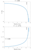 |
Fig. A.1. Relation betweenTandδfor two canonical cases.Top: Profile of T for a star with constant δ = 0.006. The crust-core boundary is indicated. Bottom: Profile of δ for a constant temperature. The dashed line represents the value that we use for the first precursor of GRB090510 (see the main text). For both panels, Eqs. (1) and (A.1) are used, and a NS pertaining to EOS SLy4 with a mass of 1.41 M⊙ is adopted. |
All Tables
Minimum tilt angle of the heavier NS in binaries with a total mass of 2.5 M⊙, such that the m = 1 g1 mode is excited to a greater extent than the m = 2 g1 mode in the sense specified in the main text.
Spin predictions, in Hz, for a variety of different resonance scenarios (i.e. for different azimuth number combinations; last four columns) and relative precursors timings (tp; first column) in a GRB095010-like system with a tilted binary (i.e. Θ ≠ 0°; though note that the angle does not affect the inertial-frame mode frequency).
All Figures
|
Fig. 1. Correlation between the frequencies of g1 and g2 modes for various EOSs and two representative values of δ (see the plot legends). For a given δ, the relations between g1 and g2 modes (Eq. (2)) are shown as bright blue lines, with the solid line representing δ = 0.005 and the dash-dot one δ = 0.01. |
| In the text | |
|
Fig. 2. Tidal overlap of m = 1 (red curve) and m = 2 (blue curve) modes as functions of inclination, Θ, in units of the tidal overlap of the l = 2 = m mode in an aligned NS (i.e. |
| In the text | |
|
Fig. 3. Strain (σ) induced by m = 2 and m = 1 g1 modes (blue and red curves, respectively) of a star spinning at ν⋆ = 30 Hz (top panel) or at ν⋆ = 63 Hz (middle panel), both with Θ = 30°, and a star spinning at ν⋆ = 63 Hz with Θ = 80° (bottom panel), all as functions of t, where the merger corresponds to t = 0. The stratification is set through δ = 0.021, as relevant for the later precursor of GRB 090510 (see Sect. 3.1). The horizontal dashed lines represent the breaking threshold; σmax = 0.04 is adopted here (Baiko & Chugunov 2018). The binary is considered to be symmetric and consists of stars of masses 1.23 M⊙ with the APR4 EOS. |
| In the text | |
|
Fig. 4. Temperature evolution due to heating by the viscous dissipation of f-mode excitations. Top: numerical (blue) and analytic (red; Eq. (20)) results obtained for a symmetric binary consisting of stars with 1.23 M⊙ and the EOS APR4. Bottom: ratio of the temperature between a varying tp and tp = −20 s corresponding to thermal ramping. In both panels, the vertical lines mark the timing of the first and second precursor of SGRB 090510, and their thickness indicates the 50 ms error for each timing. |
| In the text | |
|
Fig. 5. Derived spin of the primary (Eq. (24)) for double-precursor events with various EOSs in binaries with fixed total masses of 2.5 M⊙ and 2.8 M⊙ as functions of mass ratio q. Solid lines represent Eq. (25). |
| In the text | |
|
Fig. 6. Compactness-scaled Tvis, a, as a function of q, for three representative chirp masses, ℳ. The MPA1 EOS is used to obtain R⋆ from the stellar mass, M⋆, derived from ℳ and q. |
| In the text | |
|
Fig. A.1. Relation betweenTandδfor two canonical cases.Top: Profile of T for a star with constant δ = 0.006. The crust-core boundary is indicated. Bottom: Profile of δ for a constant temperature. The dashed line represents the value that we use for the first precursor of GRB090510 (see the main text). For both panels, Eqs. (1) and (A.1) are used, and a NS pertaining to EOS SLy4 with a mass of 1.41 M⊙ is adopted. |
| In the text | |
Current usage metrics show cumulative count of Article Views (full-text article views including HTML views, PDF and ePub downloads, according to the available data) and Abstracts Views on Vision4Press platform.
Data correspond to usage on the plateform after 2015. The current usage metrics is available 48-96 hours after online publication and is updated daily on week days.
Initial download of the metrics may take a while.