© The Authors 2023

1 Introduction

Estimating the physical properties and chemical composition of massive stars is essential to describe their wind hydrodynamics (Curé & Araya 2023) and their evolutionary status (Kudritzki & Puls 2000; Puls et al. 2008; Vink 2022), and quantitative stellar spectroscopy is a powerful tool for determining these parameters. Based on a comparison metric, this technique compares the observed spectral lines with a set of synthetic ones. These synthetic line profiles are created using a stellar atmosphere code that best suits the analysis of the star under study. However, to perform the spectral fitting, it is necessary to consider the line-broadening effect produced by the stellar rotation.

In recent years, automated fitting techniques that can carry out this quantitative spectroscopy analysis have been developed for the purpose of analyzing large samples of stellar spectra (see, e.g., Mokiem et al. 2005; Lefever et al. 2010; Simón-Díaz et al. 2011; Brands et al. 2022). These techniques have gradually replaced the traditional, time-consuming naked-eye method due to the large size of the multi-parameter space to be explored in such analysis. One of the main steps in performing a quantitative spectroscopic analysis is the determination of the line-broadening parameters (Simón-Díaz 2020). The Fourier transform method (Carroll 1933) is one of the most used approaches for deriving the projected rotational velocities (V sin i, where V is the equatorial linear velocity and i is the inclination angle of the stellar rotation axis with respect to the observer) from observed stellar lines. However, this is not the only line-broadening mechanism in stars, as thermal, radiative, collisional, microturbulent, and macroturbulent broadenings are also present in massive stars. In fact, many of them are already considered in stellar atmosphere radiative transfer calculations.

To estimate the physical parameters (e.g., T_eff, log g) of a star in the frame of quantitative spectroscopy, the non-rotating synthetic line profiles are rotationally convolved and then compared with the observed lines. The convolution is performed after measuring V sin i and the macro-turbulence speed (see, e.g., Simón-Díaz 2020; Zorec 2023).

Currently, there are many synthetic line spectra libraries that can be used in comparisons with observed spectra. However, all the models from the subset of selected synthetic spectra must be rotationally convolved to proceed with the comparison, and this is a very CPU-intensive and time-consuming task.

Instead of convolving a large number of synthetic models, in this work, we propose a method to obtain the non-rotating observed spectral line (“deconvolved spectrum”). Using this non-rotating “observed” line spectrum, we can compare it with the non-rotating synthetic spectra and select the best atmospheric model. Then, we rotationally convolve that model to fit the “real” observation.

This is a very interesting inverse problem, and it was the focus of the work of Carroll (1933). Standard tools such as Tihkonov (or Ridge) regularization (see, e.g., Christen et al. 2016) cannot be applied because the unknown function, in this problem, is the kernel of the integral expression. Alternatively, instead of solving this inverse problem, we propose to optimize a direct problem using a Gaussian sum approximation (GSA) of the kernel in the integral problem.

The method used in this paper is based on that of Carvajal et al. (2018), where a general estimation algorithm is developed using data augmentation. In this work, we adapt the proposed method in Carvajal et al. (2018), Orellana et al. (2019) and Christen et al. (2016) to estimate the non-rotational spectra.

This article is structured as follows: Sect. 2 provides the mathematical description of the proposed method. Then, in Sect. 3, Monte Carlo simulations of the proposed method applied to synthetic spectral lines are presented to show the robustness of this method. Next, in Sect. 4, some observed spectral lines are deconvolved. Finally, in Sect. 5, discussions and the final remarks are presented.

2 Effect of rotation in spectral lines

The rotational convolution of a non-rotating star profile Ι(ζ) satisfies the following integral equation for a spectral line first described by Carroll (1933) as $$O\left(\zeta \right)=K_{\text{N}}{\displaystyle {\int }_{-1}^{1}I\left(\zeta +\beta x\right)g\left(x\right)\text{\hspace{0.17em}d}x},$$(1)

where K_N is a normalization factor, ß = V sin i/c is the rotational velocity, i is the inclination angle, c is the speed of light, and g(x) represents the rotational profile that depends on the assumed limb-darkening law (see Levenhagen 2014). A summary of four different limb-darkening laws is given in Appendix A. The variable ζ is defined as $$\zeta =\frac{\lambda -{\lambda }_{\text{m}}}{{\lambda }_{\text{m}}},$$(2)

with λ being the wavelength and λ_m the wavelength of the center of the line.

3 Gaussian sum approximation approach

Knowing the ß parameter and rotational profile, g(x), the inverse problem consists of finding the non-rotational spectral line Ι(ζ) from the observed data Ο(ζ). In this work, we propose approximating the unknown spectral line Ι(ζ) with the use of a GSA (Wiener 1932), namely, $$\widehat{I}\left(\zeta |\theta \right)\approx {\displaystyle \sum _{j=1}^N{\gamma }_j\mathcal{𝒩}\left(\zeta ;{\mu }_j,{\sigma }_j^2\right)},$$(3)

where N ∈ ℕ represents the number of Gaussian functions used to approximate the spectral line, γj ∈ ℝ represents the jth weight, and 𝒩(ζ; μ_j, ${\sigma }_j^2$) represents a Gaussian function given by: $$𝒩\left(\zeta ;{\mu }_j,{\sigma }_j^2\right)=\frac{1}{\sqrt{2\pi {\sigma }_j^2}}\exp \left\{-\frac{1}{2}\frac{{\left(\zeta -{\mu }_j\right)}^2}{{\sigma }_j^2}\right\}.$$(4)

Here, σ_j is a measure of the width of the jth Gaussian function with center μ_j. Thus, the parameters to estimate are given by the vector $$\theta =\left[{\gamma }_1,{\mu }_1,{\sigma }_1^2\dots ,{\gamma }_N,{\mu }_N,{\sigma }_N^2\right].$$(5)

Then, replacing Eq. (3) in Eq. (1), we obtained: $$\begin{array}{l}\widehat{O}\left(\zeta |\theta \right)\approx K_{\text{N}}{\displaystyle {\int }_{-1}^1\widehat{I}\left(\zeta +\beta x|\theta \right)g\left(x\right)\text{\hspace{0.17em}d}x},\hfill \\ \approx K_{\text{N}}{\displaystyle \sum _{j=1}^N{\displaystyle {\int }_{-1}^1{\gamma }_j}𝒩\left(\zeta +\beta t;{\mu }_j,{\sigma }_j^2\right)g\left(x\right)\text{\hspace{0.17em}d}x}.\hfill \end{array}$$(6)

The integral in Eq. (6) was computed by utilizing the Gauss-Legendre numerical integration technique, (see, e.g., Cohen 2011), namely, $$\widehat{O}\left(\zeta |\theta \right)\approx K_{\text{N}}{\displaystyle \sum _{j=1}^N{\displaystyle \sum _{k=1}^K{\gamma }_j{\omega }_k}𝒩\left(\zeta +\beta {\varphi }_k;{\mu }_j,{\sigma }_j^2\right)g\left({\varphi }_k\right)},$$(7)

where ω_k and ϕ_k are weights and zeros of the Kth order Legendre polynomials defined by the quadrature rule. In contrast, in this work, we assume that the available measurements of O_M(ζ_τ) (τ = 1,…,M) are contaminated by measurement noise as follows: $$O_M\left({\zeta }_{\tau }\right)=O\left(\zeta \right)+{\omega }_{\tau },$$(8)

where w_τ is zero-mean Gaussian white noise with a variance of σ². In addition, we assumed that the observations are independent and identically distributed. Thus, the probability of the observed measurement O_M(ζ_τ) is given by: $$𝒩\left(O_M\left({\zeta }_{\tau }\right);\widehat{O}\left({\zeta }_{\tau }|\theta \right),{\sigma }^2\right)=\frac{1}{\sqrt{2\pi {\sigma }^2}}\exp \left\{-\frac{1}{2}\frac{{\left(O_M\left({\zeta }_{\tau }\right)-\widehat{O}\left({\zeta }_{\tau }|\theta \right)\right)}^2}{{\sigma }^2}\right\}.$$(9)

Then, the likelihood function that represents the probability of the set of measurements is given by: $$\begin{array}{l}{L}_M\left(\theta \right)={\displaystyle \prod _{\tau =1}^M𝒩\left(O_M\left({\zeta }_{\tau }\right);\widehat{O}\left({\zeta }_{\tau }|\theta \right),{\sigma }^2\right),}\hfill \\ ={\displaystyle \prod _{\tau =1}^M\frac{1}{\sigma \sqrt{2\pi }}\text{exp\hspace{0.17em}}\left\{-\frac{1}{2}\frac{{\left(O_M\left({\zeta }_{\tau }\right)-\widehat{O}\left({\zeta }_{\tau }|\theta \right)\right)}^2}{{\sigma }^2}\right\}}.\hfill \end{array}$$(10)

The log-likelihood function ℓ_M(θ) = log {L_M(θ)} reads as $$\begin{array}{l}{\ell }_M\left(\theta \right)=\log \left\{{\displaystyle \prod _{\tau =1}^M\frac{1}{\sigma \sqrt{2\pi }}\exp \left\{-\frac{1}{2}\frac{{\left(O_M\left({\zeta }_{\tau }\right)-\widehat{O}\left({\zeta }_{\tau }|\theta \right)\right)}^2}{{\sigma }^2}\right\}}\right\},\hfill \\ =-\frac{M}{2}\log \left\{{\sigma }^2\right\}-\frac{M}{2}\log \left\{2\pi \right\}-\frac{1}{2{\sigma }^2}{\displaystyle \sum _{\tau =1}^M{\left(O_M\left({\zeta }_{\tau }\right)-\widehat{O}\left({\zeta }_{\tau }|\theta \right)\right)}^2.}\hfill \end{array}$$(11)

Then, concentrating the log-likelihood function in the parameter vector θ, we obtained the following (Gouriéroux & Monfort 1989): $${\ell }_M\left(\theta \right)=-\frac{M}{2}\log \left\{\frac{1}{M}{\displaystyle \sum _{\tau =1}^M{\left(O_M\left({\zeta }_{\tau }\right)-\widehat{O}\left({\zeta }_{\tau }|\theta \right)\right)}^2}\right\}-\frac{M}{2}.$$(12)

Since log {·} is a monotonic function and by neglecting the constant terms in Eq. (12), we obtained the following concentrated function of θ: $$𝒥\left(\theta \right)=\frac{1}{M}{\displaystyle \sum _{\tau =1}^M{\left(O_M\left({\zeta }_{\tau }\right)-\widehat{O}\left({\zeta }_{\tau }|\theta \right)\right)}^2.}$$(13)

Thus, the following optimization problem is solved in order to get the deconvolved spectra $\widehat{I}\left(\zeta |\theta \right)$: $$\widehat{\theta }=\underset{\theta }{\arg \min 𝒥\left(\theta \right)}.$$(14)

The minimization problem, Eq. (14), was solved with the MATLAB function “fmincon,” using the “sqp” algorithm and setting the “Max Function Evaluations” parameter at 5000 and the “Max Iterations” parameter at 100 000. We summarize our proposed deconvolution algorithm in Table 1.

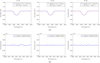Fig. 1 Absorption spectral line GSA for N = 10, 20, and 30 Gaussian functions. Top row (a): comparison of various GSA for an absorption line, employing different numbers of Gaussian functions in the approximation process. The blue solid line represents the synthetic profile, and the red dotted line represents the best GSA of 200 MC simulations. Bottom row (b): difference between the synthetic profiles and GSA. The blue solid line represents the difference between the synthetic profile and the best GSA.

4 Simulations

In this section, we present Monte Carlo (MC) numerical simulations to assess the performance of the proposed direct problem optimization. The synthetic data O(ζ₁), O(ζ₂),…,O(ζ_Μ) were generated by convolving a synthetic non-rotating spectral line, I(ζ), in Eq. (1). The synthetic non-rotating lines were calculated using the plane-parallel non-local thermodynamic equilibrium (NLTE) Tlusty¹ code (Hubeny & Lanz 1995). We computed a model with T_eff = 30 000 K and log g = 4, with solar abundance and a resolution of 0.01 Å in the range of 4500 and 4600 Å.

The simulation setup is as follows:

1. Three values of Gaussian functions N = {10, 20, 30} were considered.

2. K = 30 points (ω_k, ϕ_k) of the Gauss-Legendre quadrature were considered to solve the integral in Eq. (6).

3. Three values of V sin i = {50, 100, 200} km s⁻¹ were considered.

4. The number of MC simulations is n_MC = 200.

5. Linear limb-darkening (ϵ = 0.6, ω = 0).

The simulation setup considers. firstly, three values of Gaussian functions N = {10, 20, 30}. Secondly, K = 30 points (ω_k, ϕ_k) from the Gauss-Legendre quadrature. These points were specifically employed to solve the integral mentioned in Eq. (6). Additionally, three different values of V sin i = {50, 100, 200} km s⁻¹ were considered. Furthermore, the simulation involved a total of n_MC = 200 Monte Carlo (MC) simulations. Lastly, the simulations were done considering a linear limb-darkening with parameters ϵ = 0.6 and ω = 0.

Although linear limb-darkening was used in the simulations, the proposed method could be used with other limb-darkening laws.

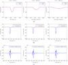Fig. 2 Absorption spectral line for V sin i = {50, 100, 200} km s−1. Top row (a): comparison of various GSA for an absorption line, employing different values of V sin i.. The blue solid line represents the synthetic profile, and the red dotted line represents the best GSA of 200 MC simulations. Middle row (b): deconvolved spectra for different values of V sin i. The blue solid line represents the non-rotated line, and the red dotted line represents the deconvolved line. Bottom row (c): difference between the synthetic profiles and GSA for different values of V sin i. The blue solid line represents the difference between the non-rotated line and the deconvolved line.

4.1 Estimation using Gaussian sum approximation

In order to evaluate the performance of the deconvolution method, a synthetic absorption spectral line was approximated using the proposed algorithm with three different values of Gaussian functions, namely, N = {10, 20, 30}. In our case, we employ the absorption line of He I λ4471 Å. This particular line is typically susceptible to the effects of rotational broadening.

The accuracy of the deconvolution was assessed by comparing the approximated absorption spectral lines with the original synthetic absorption line. Figure 1 shows the absorption spectral lines approximated using Ν = {10, 20, 30} Gaussian functions, respectively. The blue solid line represents the original synthetic absorption line, while the red dotted line is the GSA that represents the best of 200 MC simulations.

The authors found that the root mean square error (RMSE) between the original synthetic absorption line and the GSA was greater for Ν = 10 and Ν = 30 compared to Ν = 20. The best RMSE was obtained for Ν = 20, and thus the subsequent analysis in the following sections was conducted using Ν = 20 Gaussian functions. This choice represents the optimal balance between RMSE and computational time. The results demonstrate that the proposed deconvolution method accurately approximates the synthetic spectral line.

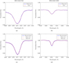Fig. 3 Deconvolution of two absorption lines for the star HD 115842. Panel a: observed He I λ 4471 Å line (blue solid line) and mean GSA (red dotted line). Panel b: observed Si III λ 4552 Å line (blue solid line) and mean GSA (red dotted line). Panel c: deconvolved He I line (blue solid line) and confidence interval (red dotted lines). Panel d: deconvolved Si III line (blue solid line)and confidence interval (red dotted lines).

4.2 Deconvolving synthetic profiles

To evaluate the performance of the proposed method, three values of V sin i = {50, 100, 200} km s⁻¹ were considered. Absorption lines were examined for each case. The results are presented in Fig. 2, which shows the GSA of the spectral lines with V sin i = {50, 100, 200} km s⁻¹. We note that for each V sin i case, the proposed method exhibits an excellent agreement between the true deconvolution (blue solid line) and the deconvolution estimated by the proposed method (red dotted line). This indicates that the proposed method is robust and accurate in deconvolving spectra with different V sin i values. Furthermore, the results suggest that the proposed method can be a reliable tool for analyzing observed spectra. However, it is important to note that the “non-rotating spectra” obtained through line decon-volution of rapidly rotating objects should be treated as an initial approximation. Figure 2c illustrates the RMSE changes according to the value of V sin i. We note that increasing the number of Gaussian functions Ν utilized in the GSA, as demonstrated in Fig. 1, can effectively reduce the RMSE of the difference.

5 Deconvolving real profiles

In this section, we apply the proposed method to He I λ4471 Å and Si III λ4552 Å lines from three stars: HD 115842, HD 47240, and HD 206267. These objects were selected to test the method’s performance.

The iacob-broad tool described in Simón-Díaz & Herrero (2014) was utilized to estimate the rotational velocity (V sin i) and the macroturbulent velocity (V_mac) through a combined methodology of Fourier transform (FT) and goodness-of-fit (GOF). This tool provides four different estimations of V sin i: the V sin i value corresponding to the first zero of the FT (red value), the V sin i and V_mac obtained from the GOF when both are treated as independent parameters (blue value), the V sin i resulting from the GOF when V_mac is fixed at zero (green value), and the V_mac resulting from the GOF when the V sin i is fixed at the value corresponding to the first zero of the FT (magenta value). In this work, we utilized the V sin i corresponding to the first zero of the FT (red value) as estimated by the iacob-broad tool to perform the deconvolution of the spectra. The specific values obtained for the stars can be found in Appendices B–D.

The spectra of HD 115842 and HD 47240 were obtained from Haucke et al. (2018), and the observations of these stars were made using the Recherche et Étude en Optique et Sciences Connexes (REOSC) spectrograph in cross-dispersion mode while equipped on the Jorge Sahade 2.15 m telescope at the Complejo Astronomico E1 Leoncito (CASLEO) in San Juan, Argentina. The spectra of HD 206267 were obtained from Nakano et al. (2012) and Wojdowski et al. (2002).

The observed line profiles were selected to encompass three distinct values of V sin i ranging from 0 to 200 km s⁻¹. By applying the proposed method to these observed line profiles of stars, the study aims to assess its effectiveness and accuracy deconvolving real observed spectra.

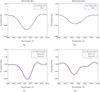Fig. 4 Deconvolution of two absorption lines for the star HD 47240. Panel a: observed He I spectral line (solid blue line) and mean GSA (red dotted line). Panel b: observed Si III line (solid blue line) and mean GSA (red dotted line). Panel c: deconvolved He I line (solid blue line) and confidence interval (red dotted line). Panel d: deconvolved Si III line (solid blue line) and confidence interval (red dotted lines).

5.1 HD 115842 star

The star HD 115842 is classified as a B0.5 Ia spectral type with a rotational velocity of V sin i = 63.5 km s⁻¹, as determined using the iacob-broad tool on the Si III line (Appendix B). The spectral lines He I λ4471 Å and Si III λ4552 Å in Fig. 3 are absorption lines. The upper panels of Fig. 3 respectively show the He I λ4471 Å and Si III λ4552 Å lines as well as the GSA. The GSA represents the mean of 200 MC simulations. In the lower panels of Fig. 3, the estimated deconvolution spectra of each line are displayed along with the 95.44% confidence interval (μ − 2σ, μ + 2σ). The deconvolution process for each spectral line was carried out using our proposed method. The results suggest that the proposed method effectively estimates the deconvolved spectra of several spectral lines.

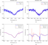Fig. 5 Deconvolution of two absorption lines for the star HD 206267. Panel a: observed He I line (blue solid line) and mean GSA (red dotted line). Panel b: observed Si III line (blue solid line) and mean GSA (red dotted line). Panel c: deconvolved He I line (blue solid line) and confidence interval (red dotted lines). Panel d: deconvolved Si III line (blue solid line) and confidence interval (red dotted line).

5.2 HD 47240 star

The star HD 47240 is a B1 Ib star with a spectral type cataloged by Turner (1976) and a rotational velocity of V sin i = 106.0 km s⁻¹, which was determined using the iacob-broad tool on the Si III line (Appendix C). Figure 4 (upper panels) displays the He I and Si III absorption lines as well as the GSA, following the same procedure as in the HD 115842 analysis, and the GSA represents the mean of 200 MC simulations. The lower panels of Fig. 4 present the estimated deconvolution spectra for each line along with the 95.44% confidence interval. The results indicate the effectiveness of the proposed method in accurately deconvolving observed spectra of both He I and Si III absorption lines.

5.3 HD 206267 star

The star HD 206267 has a spectral type of O6 (Nakano et al. 2012; Wojdowski et al. 2002) and a rotational velocity of V sin i = 186.6 km s⁻¹, as determined using the iacob-broad tool on the Si III line (Appendix D). The upper panels of Fig. 5 show the observed He I and Si III spectral absorption lines as well as the GSA. As with the previous figures, the GSA represents the mean of 200 MC simulations. In the lower panels, the deconvolution of each line is shown along with the 95.44% confidence interval. Despite the presence of measurement noise in the He I and Si III lines, the proposed method is effective in estimating the deconvolved spectra of both He I and Si III lines, as the results demonstrate. The deconvolved spectra shown in Fig. 5 exhibit spurious peaks caused by the noise in the original spectra, with an S/N of 74. Consequently, we highly recommend utilizing the proposed method for spectra with an S/N greater than 150.

6 Discussion and conclusions

This work presents a novel application for estimating the non-rotating (deconvolved) line spectra based on GSA. The proposed method uses a known rotational velocity (V sin i) obtained from the iacob-broad tool. It can directly estimate the non-rotating spectral line ($\widehat{I}\left(\zeta \right)$) from the observed one ($\widehat{O}\left(\zeta |\theta \right)$) without requiring any intermediate steps or smoothing techniques. We find that it is worth noting that the GSA method is computationally efficient, taking only a few minutes to obtain the deconvolved spectral line. However, the rotational profiles described in Appendix A do not take into account the gravitational darkening nor the stellar geometrical deformation due to high rotation (von Zeipel 1924; Espinosa Lara & Rieutord 2011). Therefore, the method should be safe to use with non-highly rotating stars.

To evaluate the effectiveness of the proposed method, we conducted an analysis using synthetic and observed lines, considering different spectral lines and numbers of Gaussian functions in the GSA (Ν = {10, 20, 30}). We found that the proposed method accurately deconvolves the spectral observed line, even in the presence of a high level of noise. However, we recommend using observed spectra with an S/Ν > 150 in order to avoid spurious peaks.

To summarize, the proposed method successfully estimates non-rotating line spectra using GSA, even in the presence of noise. In addition, this method can effectively deconvolve different spectral lines employing any limb-darkening law.

Acknowledgements

This work was partially supported by VINCI-DI PUCV through grant No 039.315/2023. J.C. Agüero and M. Coronel thank the support from ANID-Fondecyt project 1211630 and 3230398 and the Advanced Center for Electrical and Electronic Engineering (AC3E, Proyecto Basal FB0008). M. Curé, C. Arcos and I. Araya thank the support from ANID-Fondecyt project 1230131 and the continuous support from Centro de Astrofísica de Valparaíso and Centro de Estudios Atmosféricos y Astroestadística (CEAAS), Universidad de Valparaíso. Lydia S. Cidale acknowledges the financial support from CONICET (PIP 1337) and Universidad Nacional de La Plata (Programa de Incentivos 11/G160), Argentina. This project has received funding from the European Union’s Framework Programme for Research and Innovation Horizon 2020 (2014–2020) under the Marie Skłodowska-Curie Grant Agreement No. 823734.

Appendix A Carrol’s expressions in linear and nonlinear limb-darkening laws

In his early works dating back to 1928, Carroll (1928, 1933) stated that the general formulation of a line profile affected by rotational broadening could be achieved through the direct evaluation of the radiative flux, considering the following assumptions: (a) the rotation profile should be symmetric in the line of sight and (b) the limb-darkening expression is a separable function of wavelength λ and angle θ. In the following paragraphs, we denote the first and second limb-darkening coefficients appearing within the limb-darkening expressions with (ϵ, ω), which are slowly varying functions of wavelength λ, temperature, and surface gravity.. Thus, from the separability condition, we obtained the following: $$I\left(\lambda ,x,y\right)=I\left(\lambda ,\mu \right)=I\left(\lambda +\beta x\right)\varphi \left(\mu \right),$$(A.1)

where $\mu =\cos \theta =\sqrt{1-x^2-y^2}$, within which θ represents the angle formed between a point of coordinates (x, y) at the stellar surface and the line of sight; ϕ(μ) is the limb-darkening function and β = λ V sini/c.

The general expression for the outcoming flux of a star affected by rotational broadening is given by: $$O\left(\lambda \right)=K_{\text{N}}{\displaystyle {\int }_{-1}^{+1}I\left(\lambda ,\mu \right)g\left(x\right)dx},$$(A.2)

where K_N is a normalization factor and g(x) is a function dependent on the limb-darkening law, namely, $$g\left(x\right)={\displaystyle {\int }_{-\sqrt{1-x^2}}^{+\sqrt{1-x^2}}\varphi \left(\mu \right)dy}$$(A.3)

Appendix A.1 Linear limb-darkening

The linear limb-darkening law is given by (see, e.g., Levenhagen 2014, and references therein): $$\varphi \left(\mu \right)=1-\epsilon \left(1-\mu \right).$$(A.4)

Therefore, Eq. (A.2) reads $$O\left(\lambda \right)=K_{\text{N}}{\displaystyle {\int }_{-1}^{+1}{\displaystyle {\int }_{-\sqrt{1-x^2}}^{+\sqrt{1-x^2}}I\left(\lambda ,\mu \right)\left(1-\epsilon +\epsilon \cos \theta \right)dydx},}$$(A.5)

where $$K_{\text{N}}=\frac{1}{\pi \left(1-\frac{\epsilon }{3}\right)}.$$(A.6)

Developing Eq. (A.5) results in the following integral form: $$O\left(\lambda \right)=\frac{1}{\pi \left(1-\frac{\epsilon }{3}\right)}{\displaystyle {\int }_{-1}^{+1}I\left(\lambda +{\beta }_x\right)\left[2\left(1-\epsilon \right){\left(1-x^2\right)}^{1/2}+\frac{\epsilon \pi }{2}\left(1-x^2\right)\right]dx,}$$(A.7)

and the rotational profile g(x) is given by $$g\left(x\right)=\frac{1}{\pi \left(1-\frac{\epsilon }{3}\right)}\left[2\left(1-\epsilon \right){\left(1-x^2\right)}^{1/2}+\frac{\epsilon \pi }{2}\left(1-x^2\right)\right].$$(A.8)

Carroll (1933) used ϵ = 0.6 (see his Eq. 2.2).

Appendix A.2 Quadratic limb-darkening

The quadratic limb-darkening is given by $$\varphi \left(\mu \right)=1-\epsilon \left(1-\mu \right)-\omega {\left(1-\mu \right)}^2,$$(A.9)

for which we obtained the following integral equation: $$O\left(\lambda \right)=K_N{\displaystyle {\int }_{-1}^{+1}I\left(\lambda +\beta x\right)\left[2\left(1-\epsilon -\omega \right){\left(1-x^2\right)}^{1/2}+\frac{\epsilon \pi +2\omega \pi }{2}\left(1-x^2\right)-\frac{4}{3}\omega {\left(1-x^2\right)}^{3/2}\right]dx},$$(A.10)

where the normalization constant is: $$K_{\text{N}}=\frac{1}{\pi \left(1-\frac{\epsilon }{3}-\frac{\omega }{6}\right)}.$$(A.11)

Finally, the function g(x) reads: $$g\left(x\right)=\frac{1}{\pi \left(1-\frac{\epsilon }{3}-\frac{\omega }{6}\right)}\left[2\left(1-\epsilon -\omega \right){\left(1-x^2\right)}^{1/2}+\frac{\epsilon \pi +2\omega \pi }{2}\left(1-x^2\right)-\frac{4}{3}\omega {\left(1-x^2\right)}^{3/2}\right].$$(A.12)

Appendix A.3 Square-root limb-darkening

The square-root limb-darkening law is given by $$\varphi \left(\mu \right)=1-\epsilon \left(1-\mu \right)-\omega \left(1-\sqrt{\mu }\right).$$(A.13)

The governing integral equation is given by $$O\left(\lambda \right)=K_N{\displaystyle {\int }_{-1}^{+1}I\left(\lambda +\beta x\right)\left[2\left(1-\epsilon -\omega \right){\left(1-x^2\right)}^{1/2}+\frac{\sqrt{\pi }\text{Γ}\left(5/4\right)}{\text{Γ}\left(7/4\right)}\omega {\left(1-x^2\right)}^{3/4}+\frac{\epsilon \pi }{2}\left(1-x^2\right)\right]dx},$$(A.14)

where the normalization constant is given by $$K_{\text{N}}=\frac{1}{\pi \left(1-\frac{\epsilon }{3}-\frac{\omega }{5}\right)},$$(A.15)

and g(x) is: $$g\left(x\right)=\frac{1}{\pi \left(1-\frac{\epsilon }{3}-\frac{\omega }{5}\right)}\left[2\left(1-\epsilon -\omega \right){\left(1-x^2\right)}^{1/2}+\frac{\sqrt{\pi }\text{Γ}\left(5/4\right)}{\text{Γ}\left(7/4\right)}\omega {\left(1-x^2\right)}^{3/4}+\frac{\epsilon \pi }{2}\left(1-x^2\right)\right],$$(A.16)

where Γ is the gamma function.

Appendix A.4 Logarithmic limb-darkening

Finally, the logarithmic limb-darkening law is defined by $$\varphi \left(\mu \right)=1-\epsilon \left(1-\mu \right)-\omega \mu \ln \mu .$$(A.17)

It gives the integral relation: $$O\left(\lambda \right)=K_N{\displaystyle {\int }_{-1}^{+1}I\left(\lambda +\beta x\right)\left[2\left(1-\epsilon \right){\left(1-x^2\right)}^{1/2}+\frac{2\epsilon \pi +\left(\ln 4-1\right)\pi \omega }{4}\left(1-x^2\right)-\frac{\pi \omega }{4}\left(1-x^2\right)\ln \left(1-x^2\right)\right]dx},$$(A.18)

where the normalization constant is given by $$K_{\text{N}}=\frac{1}{\pi \left(1-\frac{\epsilon }{3}-\frac{2\omega }{9}\right)},$$(A.19)

and the function g(x) reads: $$g\left(x\right)=\frac{1}{\pi \left(1-\frac{\epsilon }{3}+\frac{2\omega }{9}\right)}\left[2\left(1-\epsilon \right){\left(1-x^2\right)}^{1/2}+\frac{2\epsilon \pi +\left(\ln 4-1\right)\pi \omega }{4}\left(1-x^2\right)-\frac{\pi \omega }{4}\left(1-x^2\right)\ln \left(1-x^2\right)\right].$$(A.20)

The equations (A.7), (A.10), (A.14), and (A.18) represent the convolution of a non-rotating profile Ι(λ) using the Linear, Quadratic, Square-root, and Logarithmic limb-darkening laws, respectively. Additionally, the equations (A.8), (A.12), (A.16), and (A.20), along with their respective K_N values, correspond to the rotational profiles used in the Eq. (1).

Appendix B HD 115842 star

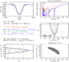Fig. B.1 Rotational velocity estimation of HD 115842 obtained using the iacob-broad tool.

Appendix C HD47240 star

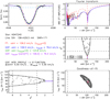Fig. C.1 Rotational velocity estimation of HD 47240 obtained using the iacob-broad tool.

Appendix D HD 206267 star

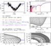Fig. D.1 Rotational velocity estimation of HD 206267 obtained using the iacob-broad tool.

References

All Tables

All Figures

Fig. 1 Absorption spectral line GSA for N = 10, 20, and 30 Gaussian functions. Top row (a): comparison of various GSA for an absorption line, employing different numbers of Gaussian functions in the approximation process. The blue solid line represents the synthetic profile, and the red dotted line represents the best GSA of 200 MC simulations. Bottom row (b): difference between the synthetic profiles and GSA. The blue solid line represents the difference between the synthetic profile and the best GSA.

In the text

Fig. 2 Absorption spectral line for V sin i = {50, 100, 200} km s−1. Top row (a): comparison of various GSA for an absorption line, employing different values of V sin i.. The blue solid line represents the synthetic profile, and the red dotted line represents the best GSA of 200 MC simulations. Middle row (b): deconvolved spectra for different values of V sin i. The blue solid line represents the non-rotated line, and the red dotted line represents the deconvolved line. Bottom row (c): difference between the synthetic profiles and GSA for different values of V sin i. The blue solid line represents the difference between the non-rotated line and the deconvolved line.

In the text

Fig. 3 Deconvolution of two absorption lines for the star HD 115842. Panel a: observed He I λ 4471 Å line (blue solid line) and mean GSA (red dotted line). Panel b: observed Si III λ 4552 Å line (blue solid line) and mean GSA (red dotted line). Panel c: deconvolved He I line (blue solid line) and confidence interval (red dotted lines). Panel d: deconvolved Si III line (blue solid line)and confidence interval (red dotted lines).

In the text

Fig. 4 Deconvolution of two absorption lines for the star HD 47240. Panel a: observed He I spectral line (solid blue line) and mean GSA (red dotted line). Panel b: observed Si III line (solid blue line) and mean GSA (red dotted line). Panel c: deconvolved He I line (solid blue line) and confidence interval (red dotted line). Panel d: deconvolved Si III line (solid blue line) and confidence interval (red dotted lines).

In the text

Fig. 5 Deconvolution of two absorption lines for the star HD 206267. Panel a: observed He I line (blue solid line) and mean GSA (red dotted line). Panel b: observed Si III line (blue solid line) and mean GSA (red dotted line). Panel c: deconvolved He I line (blue solid line) and confidence interval (red dotted lines). Panel d: deconvolved Si III line (blue solid line) and confidence interval (red dotted line).

In the text

	Fig. B.1 Rotational velocity estimation of HD 115842 obtained using the iacob-broad tool.
In the text

	Fig. C.1 Rotational velocity estimation of HD 47240 obtained using the iacob-broad tool.
In the text

	Fig. D.1 Rotational velocity estimation of HD 206267 obtained using the iacob-broad tool.
In the text

References

- Brands, S. A., de Koter, A., Bestenlehner, J. M., et al. 2022, A & A, 663, A36 [CrossRef] [EDP Sciences] [Google Scholar]
- Carroll, J. A. 1928, MNRAS, 88, 548 [NASA ADS] [CrossRef] [Google Scholar]
- Carroll, J. A. 1933, MNRAS, 93, 478 [NASA ADS] [CrossRef] [Google Scholar]
- Carvajal, R., Orellana, R., Katselis, D., Escárate, P., & Agüero, J. C. 2018, PLOS ONE, 13, 1 [Google Scholar]
- Christen, A., Escárate, P., Curé, M., Rial, D. F., & Cassetti, J. 2016, A & A, 595, A50 [NASA ADS] [CrossRef] [EDP Sciences] [Google Scholar]
- Cohen, H. 2011, Numerical Approximation Methods: Π ≈ 355/113 (Springer) [CrossRef] [Google Scholar]
- Curé, M., & Araya, I. 2023, Galaxies, 11, 68 [CrossRef] [Google Scholar]
- Espinosa Lara, F., & Rieutord, M. 2011, A & A, 533, A43 [CrossRef] [EDP Sciences] [Google Scholar]
- Gouriéroux, C., & Monfort, A. 1989, Statistique et modèles économétriques, English translation (1995), 1 (Cambridge University Press) [Google Scholar]
- Haucke, M., Cidale, L. S., Venero, R. O. J., et al. 2018, A & A, 614, A91 [CrossRef] [EDP Sciences] [Google Scholar]
- Hubeny, I., & Lanz, T. 1995, ApJ, 439, 875 [Google Scholar]
- Kudritzki, R.-P., & Puls, J. 2000, ARA & A, 38, 613 [NASA ADS] [CrossRef] [Google Scholar]
- Lefever, K., Puls, J., Morel, T., et al. 2010, A & A, 515, A74 [NASA ADS] [CrossRef] [EDP Sciences] [Google Scholar]
- Levenhagen, R. S. 2014, ApJ, 797, 29 [NASA ADS] [CrossRef] [Google Scholar]
- Mokiem, M. R., de Koter, A., Puls, J., et al. 2005, A & A, 441, 711 [NASA ADS] [CrossRef] [EDP Sciences] [Google Scholar]
- Nakano, M., Sugitani, K., Watanabe, M., et al. 2012, AJ, 143, 61 [NASA ADS] [CrossRef] [Google Scholar]
- Orellana, R., Escárate, P., Curé, M., et al. 2019, A & A, 623, A138 [NASA ADS] [CrossRef] [EDP Sciences] [Google Scholar]
- Puls, J., Vink, J. S., & Najarro, F. 2008, A & A, 16, 209 [Google Scholar]
- Simón-Díaz, S. 2020, in Reviews in Frontiers of Modern Astrophysics; From Space Debris to Cosmology, 155 [CrossRef] [Google Scholar]
- Simón-Díaz, S., & Herrero, A. 2014, A & A, 562, A135 [CrossRef] [EDP Sciences] [Google Scholar]
- Simón-Díaz, S., Castro, N., Herrero, A., et al. 2011, J. Phys. Conf. Ser., 328, 012021 [Google Scholar]
- Turner, D. G. 1976, ApJ, 210, 65 [NASA ADS] [CrossRef] [Google Scholar]
- Vink, J. S. 2022, ARA & A, 60, 203 [NASA ADS] [CrossRef] [Google Scholar]
- von Zeipel, H. 1924, MNRAS, 84, 665 [NASA ADS] [CrossRef] [Google Scholar]
- Wiener, N. 1932, Ann. Math., 1 [CrossRef] [Google Scholar]
- Wojdowski, P. S., Schulz, N. S., Ishibashi, K., & Huenemoerder, D. P. 2002, in High Resolution X-ray Spectroscopy with XMM-Newton and Chandra, ed. G. Branduardi-Raymont, 49 [Google Scholar]
- Zorec, J. 2023, Galaxies, 11, 54 [NASA ADS] [CrossRef] [Google Scholar]