| Issue |
A&A
Volume 676, August 2023
|
|
|---|---|---|
| Article Number | A95 | |
| Number of page(s) | 10 | |
| Section | Cosmology (including clusters of galaxies) | |
| DOI | https://doi.org/10.1051/0004-6361/202346093 | |
| Published online | 11 August 2023 | |
TDCOSMO
XIV. Practical techniques for estimating external convergence of strong gravitational lens systems and applications to the SDSS J0924+0219 system
1
Department of Physics and Astronomy, University of California, 95603 Davis, CA, USA
e-mail: This email address is being protected from spambots. You need JavaScript enabled to view it.
2
National Astronomical Observatory of Japan, 181-8588 Tokyo, Japan
Received:
6
February
2023
Accepted:
29
May
2023
Abstract
Context. Time-delay cosmography uses strong gravitational lensing of a time-variable source to infer the Hubble constant. The measurement is independent from both traditional distance ladder and CMB measurements. An accurate measurement with this technique requires considering the effects of objects along the line of sight outside the primary lens, which is quantified by the external convergence (κext). In absence of such corrections, H0 will be biased towards higher values in overdense fields and lower values in underdense fields.
Aims. We discuss the current state of the methods used to account for environment effects. We present a new software package built for this kind of analysis and others that can leverage large astronomical survey datasets. We apply these techniques to the SDSS J0924+0219 strong lens field.
Methods. We infer the relative density of the SDSS J0924+0219 field by computing weighted number counts for all galaxies in the field, and comparing to weighted number counts computed for a large number of fields in a reference survey. We then compute weighted number counts in the Millennium Simulation and compare these results to infer the external convergence of the lens field.
Results. Our results show the SDSS J0924+0219 field is a fairly typical line of sight, with median κext = −0.012 and standard deviation σκ = 0.028.
Key words: methods: data analysis / gravitational lensing: strong / gravitational lensing: weak / cosmological parameters / distance scale
© The Authors 2023
 Open Access article, published by EDP Sciences, under the terms of the Creative Commons Attribution License (https://creativecommons.org/licenses/by/4.0), which permits unrestricted use, distribution, and reproduction in any medium, provided the original work is properly cited.
This article is published in open access under the Subscribe to Open model. This email address is being protected from spambots. You need JavaScript enabled to view it. to support open access publication.
1. Introduction
One of the most important problems in modern cosmology is the so-called Hubble tension: the name given to an apparent discrepancy between the value of the Hubble constant (H0) inferred from the Cosmic Microwave Background assuming the standard Λ-CDM cosmological model (e.g., Planck Collaboration VI 2020), and the value inferred from Cepheid-calibrated Type Ia supernovae (e.g., Riess et al. 2021). The solution to this discrepancy may involve unknown systematics, new physics, or some combination of the two. Work on the resolution is ongoing, but having independent methods for inferring the value of the Hubble constant is critical for solving the problem. Such methods include using the tip of the red giant branch to calibrate supernovae (Freedman et al. 2019) and BAO+BBN (Cuceu et al. 2019), among others. Here we consider Time Delay Cosmography, which uses strong gravitational lensing of time-variable sources (usually a quasar) to infer the value of H0.
TDCOSMO is an international collaboration which aims to use strong gravitational lensing to infer the value of H0 with sub-percent precision. A typical lens in the TDCOSMO sample involves a source quasar being strongly lensed by a foreground galaxy, producing four images. When the quasar’s luminosity varies, this variation appears in each of images at different times. The “time delay” between two images depends on the mass distribution of the lens, and the time-delay distance:
 (1)
(1)
Where zd is the redshift of the lensing galaxy (or “deflector”), and Dd, Ds, and Dds are the angular dimater distances to the deflector, source, and from the deflector to the source, respectively.
Given a model of the lens and a measurement of the time delays, it is possible to infer the time-delay distance and therefore H0. For J0924, a model was presented in Chen et al. (2022), but a sufficiently accurate time delay has not yet been measured.
When analysing a strong lens, there are a number of sources of uncertainty that propagate to the final inferred value of H0 (see Millon et al. 2020, for a more complete overview). Among these are so-called environmental effects: gravitational bodies besides the primary lens that affect the lensing observables and, by proxy, the inferred value of H0. Accounting for these effects is crucial in improving the precision of the inferred measurement. Broadly speaking we treat weak perturbers differently from strong ones, with the difference being determined with the “flexion shift” formalism (see for example Buckley-Geer et al. 2020; Sluse et al. 2019; McCully et al. 2017).
In this paper, we focus on the techniques for inferring the cumulative effect of all weak perturbers along the line of sight to the source quasar. This is done by comparing the field of interest to some suitably large reference field, with the goal of estimating the relative density of the field as compared to the universe at large. This is a purely statistical analysis. In this paper, we will discuss the current state of this technique, apply it to the field around the SDSS J0924+0219 lens system (hereafter J0924), and discuss how it might be iterated upon in the future. The cumulative effect of all weak perturbers is parameterized by the external convergence, denoted κext.
While controlling uncertainties on individual lens systems is crucial, the precision of the measurement can be improved by including many lenses in the final inference. Of course, this is much easier said than done as the amount of work required to fully analyze a single lens is significant. However in the modern era of data-driven astronomy, the amount of available data is increasing by orders of magnitude and developing tools for efficiently analyzing these datasets is a top priority. To that end, we introduce lenskappa, a new package designed specifically for the types of environment analysis discussed in this paper, but with broader applications. lenskappa is built on top of heinlein, a data management library designed for use with large astronomical survey datasets. At present heinlein and lenskappa support Subaru Hyper Suprime Cam Strategic Survey Program (HSC-SSP; Aihara et al. 2019), the Dark Energy Survey, and the CFHT Legacy Survey.
This paper is organized as follows: In Sect. 2, we outline the fundamentals of Time Delay Cosmography and the basic process used to compute a value of κext for a generic lens system. In Sect. 3 we discuss the datasets used in our analysis, and introduce lenskappa. In Sect. 4, we report the results of our analysis of the J0924 field obtained using lenskappa. In Sect. 5 we discuss our results and look forward to later work.
2. Summary of the technique
In this section, we introduce the basics of time delay cosmography and describe the technique we use to estimate κext for a generic lens system. For a more complete overview, we refer the reader to Treu & Marshall (2016) and Birrer et al. (2022).
2.1. Fundamentals of time delay cosmography
Time delay cosmography focuses on strong lensing of time-variable sources, usually a quasar. As the luminosity of the source varies, this variation appears in each of the several images of the source, but not at the same time. The time delay between any two images can be written as follows:
![Mathematical equation: $$ \begin{aligned} \Delta t_{ab} = \frac{D_{\Delta t}}{c}\bigg [ \frac{(\overrightarrow{\theta _a} - \overrightarrow{\beta })^2}{2} - \frac{(\overrightarrow{\theta _b} - \overrightarrow{\beta })^2}{2} - \psi (\overrightarrow{\theta _a} ) + \psi (\overrightarrow{\theta _b})\bigg ], \end{aligned} $$](/articles/aa/full_html/2023/08/aa46093-23/aa46093-23-eq2.gif) (2)
(2)
where  represents the angular position of an image on the sky,
  represents the actual (unobservable) angular position of the source on the sky, and ψ is the scaled lensing potential. The first two terms are a result of the different distances traveled by the light for the two images, while the later two terms are the difference in the Shapiro time delay. The goal of our analysis is to infer the time-delay distance (see Eq. (1)). Using measurements of the time delay combined with a robust model of the lensing galaxy it is possible to measure the time delay distance and, therefore, the Hubble constant.
This picture is complicated when considering perturbers outside of the primary lens. We quantify the effect of all weak perturbers along the line of sight with κext, which is known as the external convergence of the field. In general, convergence results in a magnification (or demagnification) of the image. However this effect is not directly observable as the true angular size of the source is not known. To compute κext we compare the statistical properties of the lens field with statistical properties of some suitably large reference field. Usually κext is of order 10−2, with positive values representing a field that is slightly overdense as compared to the universe at large, and negative values corresponding to an underdense field. In general, κ at a given position is directly related to the total gravitational potential at that position.
 (3)
(3)
Assuming κext can be measured, it serves as a correction factor to the computed value of the time delay distance:
 (4)
(4)
where  represents the uncorrected value of the time delay distance. This propagates directly to the inferred value of the Hubble constant by
 (5)
(5)
We see therefore that in the absence of the appropriate corrections, the inferred value of Hubble constant will be biased towards higher values in an overdense field, and lower values in an underdense field.
The external convergence is one of two primary weak lensing parameters, the other being the external shear (denoted γext). While κext magnifies the image, γext stretches it. Because the intrinsic size and luminosity of the source object is not know, it is not possible to directly observe κext. While the external shear at any one point in a given field is a two-dimensional quantity, we make use only of the overall strength of the external shear in our analysis.
We now review the techniques we use to compute the value of κext for a generic lens system.
2.2. Relevant perturbers in the line of sight
To start, we identify objects along the line of sight that contribute to κext. In this type of analysis, we do not treat each perturber individually, but instead consider the statistics of the entire field. However, there are cases where galaxy groups appear along the line of sight and must be taken into account explicitly (see for example Sluse et al. 2019; Fassnacht et al. 2006).
The first step in determining the value of κext is determining the relative density of the lens field as compared to some suitable reference field. The reference field should be large enough to avoid sampling bias. Ideally the data for the reference field and lens field are taken by the same instrument and processed by the same analysis pipeline. This turns out to be the case for the analysis of J0924 discussed later in this paper, but will not be true in general.
Once the appropriate data are in hand, it is important to consider which objects should be used in the comparison. It is important to set a magnitude cut that will remove objects too close to the detection limit of the instrument for photometry to be reliable, while still leaving enough data to make robust estimates of the relative density. Previous work (see Collett et al. 2013) has suggested that i < 24 represents a good limit. Additionally, we cut out all objects with a redshift greater than the redshift of the source quasar, as these objects will not affect the path of the light as it travels from the quasar to our telescopes.
Broadly speaking, this analysis only considers weak perturbers. Strong perturbers are generally modeled explicitly. To separate these, we use the flexion shift formalism, first proposed in McCully et al. (2017). The flexion shift of an object is given by
 (6)
(6)
where θE and θE, p are the Einstein radii of the main lens and perturber respectively, and θ is their angular separation. The quantity f(β) is given by
 (7)
(7)
where
 (8)
(8)
where Ddp, Ds, Dp, and Dds are the angular diameter distances from the deflector to the perturber, to the source, to the perturber, and from the deflector to the source. The flexion shift roughly measures the perturbations to the images of the source due to 3rd order terms from the perturber. McCully et al. (2017) recommend using Δ3x > 10−4 arcsec to avoid ensure a < 1% bias on H0 from perturbers.
2.3. Weighted number counts of lens field
As a first approximation, we expect the greatest contribution to κext from massive objects close to the center of the line of sight. The primary mass contribution in any line of sight will be dark matter halos, but these are not directly observable. To quantify the contribution from these weak perturbers, we compute weighted number counts of the visible structures (i.e., galaxies) in the lens field as compared to a large number of reference fields. This technique has been used extensively in previous work (Rusu et al. 2017; Buckley-Geer et al. 2020; Greene et al. 2013; Suyu et al. 2010). To do this, we select a region of interest around the lens and compare it to a large number of identically-shaped fields selected at random from the reference survey. At each step, we compute the ratio of the weighted number counts for the galaxies in the lens field to the identical statistic computed in the given reference field. At each step, the value of the weight is therefore:
 (9)
(9)
Where i indexes the reference fields, j indexes the galaxies in a given field, and w is the value of the weighted statistic for the given galaxy.
Following Rusu et al. (2017) we also consider a second style of weighting that improves our results. Instead of summing the value of weights for all objects in the field, we instead compute the weight for a given field as  where ni is the number of galaxies in the given reference field and
  is the median value of the weight for all galaxies in the reference field. Doing this helps avoid situations where single objects dominate the sum in a particular line of sight. This is especially important for weights involving stellar mass and the inverse separation. In this scheme, the value of the weight for the given reference field is therefore
 (10)
(10)
There has been discussion in the literature about which are the best weights to consider for the most robust determination of kext (Greene et al. 2013; Rusu et al. 2017, 2019). In this work, we only consider a subset of the weights considered in previous works (see Table 1).
Weighted number counts considered in this work.
2.4. Weighted number counts in simulated data
In order to determine the posterior distribution of κext for the given system, it is necessary to compare the weighted number counts to similar counts obtained from a reference field for which κext is known. We use a simulated dataset for this purpose. The simulation must contain several components in order to be suitable for this analysis. First, it must contain catalogs of galaxies with known luminosity and redshift. Second, values of the external convergence must be measured at a suitably large number of points to be representative of the universe at large. Rusu et al. (2017) examined possible biases from inferring κext using the number counts method in the Millennium Simulation, and found these methods produced a good estimate of κext. We discuss our choice of simulation further in Sect. 4.3. Because this technique involves ratios, much of the dependence on the simulation’s underlying cosmological parameters should cancel out. However, ensuring this would require a second simulation with the attributes described. An exciting development in this space are the initial results from the MillenniumTNG (Hernández-Aguayo et al. 2023). Full weak-lensing convergence maps are planned, but not yet available.
2.5. From weighted number counts to κext
We now have weighted number counts for the lens field itself and for a large number of fields in a simulated dataset, each of which is associated with a value of κext. We seek to compute p(κext|d): the probability distribution of κext given the data. We can replace this with the joint probability distribution of κext and the data as follows:
 (11)
(11)
After some work it can be shown (see Rusu et al. 2017)
 (12)
(12)
where p(W|d) is the probability distribution of given weighting scheme given the data, and psim(κext|W) is the probability distribution of kappa in the simulated dataset, given a particular value of the weight. Here, it is assumed that the simulated dataset is the correct prior for the observable universe. In other words, that it correctly relates values of weights to values of κext.
Additionally, a constraint on κext based on γext can be included, which accounts for the expected correlation between these two values. This provides a prior on κext that can meaningfully affect the final result.
In previous work (e.g., Rusu et al. 2017), this full probability distribution for each weight p(W|d) was replaced by a normal distribution centered on the median of the full weight distribution, with a width determined by examining measurement uncertainties. In practice, this width was much smaller than the width of the actual distribution. This is cheaper computationally, but ignores covariance between the various types of the weights. While the increase in computation time is significant, the majority of the important decisions in the analysis are made when we compute weighted number count ratios, and using this method does not meaningfully increase our time-to-result.
Since all the individual weights are measured at the same sequence of randomly-drawn fields, we can construct a full m-dimensional probability distribution p(Ws|d) = p(Wn, W1/r, …|d) where m is the number of weights being considered. We then explore this probability distribution when implementing the formalism described above. Formally, the posterior on κext becomes:
 (13)
(13)
when computing this quantity, we split the m-dimensional probability distribution into 200mm-dimensional bins. We have also tested this procedure 100m bins and see consistent results for the J0924 field. With significantly more bins, the computational time balloons and the number of fields in each bin drops significantly, even near the center of the distribution. The value of p(Ws|d) is simply the number of lines of sight in the reference survey that fall in this bin divided by the total number of lines of sight being considered. Given the large numbers of lines of sight we consider, the distributions are smooth and it may be possible to model them explicitly and forgo binning entirely, but we save this for a future analysis. The exception to this is the pure unweighted number counts in a 45″ aperture, due to the fact that the “weight” is integer valued and the number of galaxies in the aperture is relatively modest.
For pMS(κext|Ws) we construct a histogram of the measured values of κext for all lines of sight from the Millennium Simulation that fall within the given bin, normalized by the number of lines of sight in the bin. Without this normalization, κext values near the mean of the Millennium Simulation will always be weighted more heavily because there are comparatively more of them.
The inputs to our analysis code include the full weight distributions for the lens field, the weights computed from the Millennium Simulation, and the κext maps for the Millennium Simulation for the source redshift. We iterate over the probability distribution discussed above, computing a histogram of the values of κext in each m-dimensional bin. The overall histogram is the sum of these histograms, weighted by the value of the weight distribution in that bin.
3. Datasets, automation, and lenskappa
As with many areas of astronomy, time-delay cosmography is grappling with datasets that are growing at unprecedented rates. There are dozens of known quad lenses which may be suitable for cosmographic analysis, but a full analysis has only been completed on a small fraction of them. Techniques for increasing the rate of analysis are therefore crucial to the continued success of the technique.
While there are many open science questions in Time Delay Cosmography, much of the solution to the rate problem lies in software engineering rather than astronomy. When building for this kind of analysis, we keep three key questions in mind:
-
What is the minimum amount of data required to complete a particular analysis step with sufficient precision?
-
How much of the analysis can realistically be automated?
-
Do we expect the analysis techniques to change significantly in the future?
The answer to these questions may not be independent. For example, a pipeline that uses less data at the expense of increasing uncertainties on individual systems may be tolerable if it significantly increases the rate at which these systems can be analyzed. The third question is also important. Writing flexible software packages that can easily be updated as analysis techniques evolve usually increase the time to first result, but substantially decrease average time to result in the long run.
Among the various steps required to fully analyze a lens system, the number counts technique discussed in this paper is likely the most straightforward to automate. It is mostly statistical, and the most difficult computational challenge is efficiently filtering a large dataset by location. Furthermore the survey datasets used in this analysis are quite robust, and many of the lens systems fall within one or more survey footprints. This makes the first question a non-issue, at least for a significant fraction of the lenses.
To that end, we introduce lenskappa1 and heinlein2. The goal of lenskappa is to build a tool capable of automating environment analysis to the greatest extent possible, while still providing sufficient flexibility to allow us to iterate on our current methods. lenskappa is in turn built on top of heinlein, which serves as a high-level interface to locally stored astronomical datasets. When computing weighted number counts in lenskappa, the core weighting loop consists of:
-
Select a region of interest from a large survey.
-
Retrieve object catalog and auxiliary data for the region.
-
Compute interesting quantities, using the data retrieved for the region.
A single iteration of this loop is represented in Fig. 1.
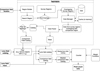 |
Fig. 1. Flowchart representing the process of computing a weighted count ratio given a location in a reference survey. Most of the heavy lifting is done in heinlein which is optimized for analyses involving repeated queries in a particular area. |
heinlein handles the middle step of this loop. It provides high-level routines for storage, retrieval, and filtering of large survey datasets, as well as intuitive interfaces for interaction between data types (for example, applying a bright star mask to a catalog). heinlein can perform a 120″ cone search in the HSC dataset in around 1.5 s, without requiring the data be pre-loaded into memory. For later queries of nearby locations, the speed is improved by more than an order of magnitude through caching. This makes heinlein suitable both for interactive use and for the kind of analysis done in lenskappa.
With data retrieval optimized, lenskappa focuses on using these datasets to perform interesting analyses. Although we built lenskappa for the kind of analyses discussed in this paper, it is designed to be flexible and permit users to define new and interesting analyses without modifying the core code.
lenskappa includes several features to facilitate this including:
-
High-level API for defining analyses.
-
Plugin architecture for adding new capabilities without modifying the core code.
-
Automatic support for any dataset supported by heinlein.
Analyzing modern astronomical survey datasets at scale. One of the big challenges in doing analyses on these kinds of datasets is the need for the computing environments to be close to the data whenever possible. Querying over the internet is useful for assembling datasets, but is not a particularly good solution when analyzing a dataset at scale. Many researchers will not have access to sufficient storage to store these datsets, and it is impractical to expect individual survey teams to provide computing resource for general use. The size of these datasets will enable next-generation analyses, but only with the development of next-generation tools running at scale, which will require computing infrastructure that may not be readily available to many researcher.
We support using cloud computing services to fill this gap. Commercial providers have expanded and matured by leaps and bounds over the last decade, and routinely handle storage and analysis tasks on datasets orders of magnitude larger than the ones being discussed here. Additionally, cloud computing technologies are significantly more accessible then on-premise technology: they require far lower startup costs and can be quickly scaled (to accommodate more users, or bigger jobs) without the bottlenecks that slow down the expansion of on-premise infrastructure.
It is also possible to use cloud solutions as a supplement to already-existing on premise solutions. Holzman et al. (2017) demonstrated this by analyzing data from the Compact Muon Solenoid experiment at massive scale.
In the future, we plan to develop lenskappa and heinlein tools that could be easily deployed onto services like these, providing quick and easy access to large survey datasets in addition to techniques for processing and analyzing that data. The datasets would be stored in the cloud, allowing users to deploy their analyses without worrying about the connection to the underlying dataset. Such an approach has been demonstrated by Kusnierz et al. (2022), which enabled serverless access to ROOT for quick analysis tasks on high energy datasets without the user having to manually retrieve the data. With some work, heinlein will enable this type of analysis by serving as a bridge between computing infrastructure (which could be managed by individual researchers) and the underlying data lake (which could be managed by the survey team). Abstracting away data retrieval will allow researchers to focus on what matters most: designing the analyses they wish to perform and interpreting results.
4. Analysis of SDSS J0924+0219
In this section, we discuss the analysis of the J0924 system, as performed by lenskappa.
4.1. The lens field
SDSS J0924+0219 is a quadruply lensed quasar first reported in Inada et al. (2003). The quasar itself is at redshift z = 1.523, while the lensing galaxy is located at z = 0.384 (Eigenbrod et al. 2006). Quadruply lensed quasars are particularly valuable for cosmographic analysis because it is in principle possible to measure 12 different time delays, though only three of these are independent. An image of the field can be seen in Fig. 2. This system was modeled in Chen et al. (2022).
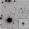 |
Fig. 2. Field around SDSS J0924, shown in HSC i-band. The red rings represent 5″, 45″ and 120″ apertures respectively. Note the presence of the bright star in the lower left that is included in the 120″ aperture, but not the 45″ aperture. Bottom right: close up view of the lens system. |
One particularly important feature of the lens field is the bright star located in the lower left. The star covers a reasonably large fraction of the overall area in the 120″ aperture, undoubtedly covering several background objects and making photometry for objects very near it unreliable. We apply techniques that have previously been used in this kind of analysis to correct for this. This technique is discussed in more detail in Sect. 4.2.
The lens field falls within the Subaru Hyper Surpime-Cam Strategic Survey Program footprint, and full color information is available for all objects in the relevant catalogs. We use these catalogs, including photometric redshifts, for all objects inside the field. Additionally we use the bright star masks and photometric redshift PDFs provided by the HSC team.
Our analysis follows the same outline discussed in Sect. 2. We discuss the details particular to this lens field below.
4.2. The HSC survey and weighted number count ratios
The Hyper Suprime-Cam Subaru Strategic Survey is a large survey program, aiming to cover roughly 1400 deg2 of sky in five photometric bands down to mag ∼26, with deeper coverage expected in smaller regions of the sky (Aihara et al. 2017). We base our analysis on the roughly 400 deg2 that had coverage in all five bands as of the second data release (Aihara et al. 2019). Data release 3 was made available while this paper was in preparation, but we do not consider it here.
The HSC Survey is a natural choice for a comparison dataset for this system because the J0924 field itself falls within the survey footprint. We therefore have both robust and comparable photometry. When computing weighted number count ratios, the basic approach is identical to the one outlined in the Sect. 2.3, with some specific adjustments:
We use objects with r_extendness_value = 1.0, which selects galaxies. Bosch et al. (2017) demonstrate that their algorithm for computing this quantity does a reasonably good job of selecting galaxies, though it may incorrectly classify some galaxies as stars, and vice versa. However we note that the HSC-wide survey was intentionally selected to enable cosmological analyses by being in regions that are away from the galactic plane and low on dust extinction (Aihara et al. 2017). This, combined with robust bright-star masks and our large sample size ensures unmasked stars do not significantly impact the final weighted number count ratios.
The full photometric redshift PDFs for all objects in the data release have been made available by the HSC team (Nishizawa et al. 2020). They use two separate fitting algorithms, and results from both algorithms are included in the catalog. We compute weighted number count ratios using both sets of redshifts, and do not find a meaningful difference between the resultant distributions. As such, we use the “Demp” redshift and stellar masses for our analysis (Hsieh & Yee 2014; Tanaka et al. 2017).
When computing weighted number counts, we remove all objects closer than 5 arcsec from the center of the field following Rusu et al. (2017). Objects this close to the center of the field are typically explicitly included in the mass model of the lens, and so we also remove them from the comparison fields to avoid biasing results.
The HSC survey team makes available masks that represent areas of the sky where photometry may be unreliable or lacking due to the presence of bright stars (Coupon et al. 2017). This is particularly important in our field due to the presence of the bright star that can be seen in Fig. 2 When iterating over the reference survey, we retrieve the bright star masks for each region being considered. We apply both these masks and the masks for the lens field itself to both catalogs at each weighting step. Doing this ensures that results are not biased if a given field in the reference survey has significantly more or less of its area covered by bright star masks. This procedure was first used in Rusu et al. (2017).
The 400 deg2 of sky we consider here is separated into seven disconnected regions. Initially, we computed weighted number count ratios in five of these regions. This produces nearly-identical distributions, with the difference between the lowest and highest median being 0.1σ the standard deviation of the distribution, suggesting our fields are large enough to to avoid sampling bias. Based on this, we restrict our subsequent analysis to 135 deg2 of the W05 region. For each combination of aperture and limiting magnitude, we compute weighted count ratios at 100 000 randomly selected fields.
4.3. Millennium Simulation
The Millennium Simulation (Springel et al. 2005) is a dark matter only simulation split into 64 4 × 4 deg2 fields. After the original run was completed, synthetic galaxy catalogs were painted into the resultant halos by several teams. Following (Rusu et al. 2017) we use the semi-analytic catalogues of De Lucia & Blaizot (2007). Additionally, Hilbert et al. (2009) split each 4 × 4 deg2 field into a grid of 4096×4096 points and used ray tracing to compute convergence and shear at each of these points in 63 redshift planes. These, combined with its large size, makes it an excellent choice for our analysis. In our analysis, we use redshift plane 36 with z = 1.504.
First, we compute the weighted number counts at a large number (order 106) of equally spaced grid points in the Millennium simulation. For the 45″ aperture, we place the fields 90″ apart (snapped to the nearest grid point), while for the 120″ aperture we place fields 60″ apart. Both cases result in over 1.5 million lines of sight across the simulation, each of which has an associated value of κext and γext This differs from the same calculation for the lens field itself in a key way: the values reported are the total value of the weights at every point considered, rather than a ratio of values. To normalize, we divide weighted number count in each field by the median value for all lines of sight in our sample. The median value of the resultant distribution is therefore unity.
A key difference between the synthetic catalogs and the real data from the HSC survey is that in the Millennium Simulation catalog redshifts are exact. In previous work (e.g., Rusu et al. 2017) this difference was accounted for by computing photometric redshifts for all objects in the Millennium Simulation, using the same pipeline that was used to compute the photometric redshifts in the comparison dataset. We are unable to use this technique in this case because the HSC survey photo-z pipelines are not publicly available as of the preparation of this paper. Instead, we download the full catalog of training data used by the HSC. These are galaxies for which spectroscopic redshifts are available. We divide the objects in the test dataset into redshift and magnitude bins. For each galaxy in a bin, we compute the offset in the central value of the redshift (zphot − zspec), and take the median of these as our estimate of the redshift bias in that bin. Additionally we take the median value of σz (as reported by the HSC photometric redshift pipeline) for all photometric redshifts in that bin. We take the median value of σz as our estimate of photometric redshift uncertainty. For each object in the Millennium Simulation catalog, we construct an artificial photemetric redshift PDF. The center of the distribution is the “actual” redshift of the object, offset by the amount computed previously for the appropriate bin. The width of the distribution is the value of σz computed for the same bin.
At each weighing step in the Millennium Simulation, we then sample from these “photometric redshift” PDFs when computing weighted number counts. For each line of sight, we sample from each of these PDFs 50 times. This produces 50 separate catalogs (all with slightly different values for object “redshifts”), and we compute weighted number counts for each one. We find that this process produces no meaningful change to our final inference for κext, even when a weight that depends on the redshift is taken into account. However this process massively increases the amount of data output by our code, and therefore significantly increases the amount of time required to do the final inference on κext. This does suggest that photometric redshift uncertainties do not have a significant impact on the inferred value of κext. However, we plan to do a more thorough analysis with real photometric redshift PDFs before coming to any conclusions.
5. Results and discussion
Our weighted number counts for the lens field include a total of five weights (wn, w1/r, wp, wz, wz/r), two apertures (45″ and 120″), two limiting magnitudes (23 and 24), and two summing techniques (pure sum and medians). For brevity, we report only the medians of these distributions in Table 2. The full distributions, along with the analysis code used to produce the posterior distributions for κext can be found online3. A visual catalog of the objects in the field and their relative weights can be seen in Fig. 3.
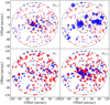 |
Fig. 3. Location and relative weights of all galaxies with z < zs. The black circles represent the 45″ and 120″ apertures respectively. Blue objects are those with i < 23, while red objects are those with 23 < i < 24. The relative weight of the object is represented by the size of the dot, down to a minimum value set for clarity. |
Median of weighted number counts for SDSS J0924 Field.
The weighted number count ratios suggest the SDSS J0924 field is mildly overdense as compared to the universe as a whole. This overdensity is significantly more obvious when considering the 45″ aperture. This is quite reasonable; as the size of the aperture increases, the density of field will approach the density of the universe as a whole. See Fig. 4 for an overview of the weights considered in this work.
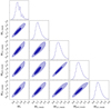 |
Fig. 4. 2D histograms of for each possible pair of the weight number count ratios considered in this work. The weights we were computed with a 45″ aperture and limiting magnitude i < 24. The jagged histogram for the unweighted counts is due to the relatively small number of galaxies in an aperture of this size. The inner and outer contours represent 68 and 95% confidence intervals, respectively. |
It is however less obvious why the value of the weights seem to depend on the limiting magnitude, with the median values for i < 23 being significantly higher than for i < 24. This may suggest that the quality of the lens field catalog is poor below magnitude 23, We remind the reader that the 5″ region around the lens itself is masked when computing weighted number counts.
Based on the above, we would expect our final value of κext to be somewhat positive. However the strength of the external shear of the field, reported in Chen et al. (2022) is  . This places it significantly below the median (and, in fact, mean) for all lines of sight in the Millennium Simulation. For each combination of limiting magnitude and aperture we compute κext for a number of different combinations of weights:
-
Pure (unweighted) number counts, combined with each of the remaining weights individually.
-
Pure number counts and inverse distance weights, combined with each of the remaining weights individually.
-
For each of the above cases, we run the kappa inference both with and without the constraint from γ.
The number count ratios used for this analysis are listed in Table 2. We do not mix distributions obtained using our two different weighting techniques.
We also repeat this for each while using the median weighting scheme rather than the sum scheme. All together, this leaves us with 112 individual histograms for the value of kappa.
We find that the choice of specific weights is less important than the number of weights being considered. In all cases, inferring κext with three weights instead of two tightens the resultant distribution, but does not significantly affect the central value. Rusu et al. (2017) found best results when combining wn and wr with one additional weight and the constraint from γext. The central value of the distribution does not change meaningfully based on the choice of the third weight, but we find slightly tighter constraints when using wp.
We also find that results are consistent between apertures, but find that a brighter value of the limiting magnitude results in a noisier posterior on κext. Because so many objects fall between magnitude 23 and 24, removing these objects results in significantly noisier weighted number counts which translate to the final inference on κ.
Considering only γ as a constraint leads to a median value on κext of −0.015. As a result, including γext as a constraint significantly lowers the central value of our distributions, though it also tightens the distribution. However we note this shift is fairly modest as compared to the width of the distribution. This is similar to the result seen in Rusu et al. (2017), though in that case the inferred value of the shear was significantly closer to the median in the Milennium Simulation of 0.028, and the shift of the central value was not as significant. We find our tightest constraints on κext through a combination of wn, w1/r and wp combined with constraints from γext. This leads us to a final value of κext of −0.012 with a width σκ = 0.028. Without the constraint from γext, we obtain a median value of 0.012 with σκ = 0.053. Full posteriors for these combinations can be found in Fig. 5.
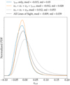 |
Fig. 5. Comparison of smoothed posterior on κext for wn + wr + wp without γext, wn + wr + wp with γext, and γext alone. For distributions that depend on weighted number count ratios, we use a 45″ aperture with i < 24. |
6. Conclusions and future work
In this paper, we have discussed the current state of the line of sight number counts technique for environment analyses in time delay cosmography. We have introduced two main improvements to previous iterations of the analysis. First, our packages lenskappa and heinlein make designing and running these analyses much quicker than before, in addition to making it much simpler to add additional survey datasets. This will accelerate the pace of future analyses, and enable population-level analyses of lens environments. Additionally, we have made use of the entire distributions of weighted number counts, which accounts for covariance between weights and is generally more robust than just exploring a small region around the medians. We have applied these techniques to the J0924 field, and found that this field is a fairly typical line of sight, with a slightly negative median value of κext.
6.1. Future development of lenskappa
Our primary goal for this project has been to build a software tool that can quickly and reliably analyze weak perturbers along lines of sight to strong gravitational lenses. We have accomplished this goal, but we plane to extend the capabilities of lenskappa to include tools for analyzing strong perturbers and coherent structures (such as galaxy groups). These objects must be handled individually, and require very different analysis tools. However we see a significant advantages to being able to do full environment analyses within a single software package.
6.2. Future analyses
Leveraging the capabilities of lenskappa, we hope to better understand lines of sight to gravitational lenses on a population level. Fassnacht et al. (2010) and Wong et al. (2018) have shown that lenses seem to fall in preferentially overdense lines of sight, but that this overdensity seems to be confined to the immediate surroundings of the lens itself. Lenskappa gives us the tools to perform these population-level analyses quickly, with the freedom to adjust and re-run the analysis as needed. As a first step, we hope to complete an analysis with 4–5 new lens systems, as well 2–3 systems that have previously been analyzed to check our results.
As an additional check, we would like to analyze a large number of non-lens lines of sight. This would ensure there are no biases introduced by comparing distributions based on real galaxy catalogs to those obtained from the synthetic catalogs in the Millennium Simulation.
Recently, Park et al. (2022) demonstrated the use of Bayesian Graph Neural Network to estimate the value of κext in a simulated dataset. Their method out-performs a simplified version of the analysis performed hear that uses only a single weight. Further work may demonstrate the ability of the technique to match or even outperform the weighted number counts technique, but a more complete comparision will need to be performed to assess this.
Acknowledgments
P.W. and C.D.F. acknowledge support for this work from the National Science Foundation under Grant No. AST-1907396. P.W. thanks Liz Buckley-Geer, Anowar Shajib, and Simon Birrer for useful discussions throughout the preparation of this manuscript.
References
- Aihara, H., Arimoto, N., Armstrong, R., et al. 2017, PASJ, 70, S4 [NASA ADS] [Google Scholar]
- Aihara, H., AlSayyad, Y., Ando, M., et al. 2019, PASJ, 71, 114 [Google Scholar]
- Birrer, S., Millon, M., Sluse, D., et al. 2022, Space Sci. Rev., submitted [arXiv:2210.10833] [Google Scholar]
- Bosch, J., Armstrong, R., Bickerton, S., et al. 2017, PASJ, 70, S5 [NASA ADS] [Google Scholar]
- Buckley-Geer, E. J., Lin, H., Rusu, C. E., et al. 2020, MNRAS, 498, 3241 [NASA ADS] [CrossRef] [Google Scholar]
- Chen, G. C.-F., Fassnacht, C. D., Suyu, S. H., et al. 2022, MNRAS, 513, 2349 [NASA ADS] [CrossRef] [Google Scholar]
- Collett, T. E., Marshall, P. J., Auger, M. W., et al. 2013, MNRAS, 432, 679 [NASA ADS] [CrossRef] [Google Scholar]
- Coupon, J., Czakon, N., Bosch, J., et al. 2017, PASJ, 70, S7 [NASA ADS] [Google Scholar]
- Cuceu, A., Farr, J., Lemos, P., & Font-Ribera, A. 2019, J. Cosmol. Astropart. Phys., 2019, 044 [CrossRef] [Google Scholar]
- De Lucia, G., & Blaizot, J. 2007, MNRAS, 375, 2 [Google Scholar]
- Eigenbrod, A., Courbin, F., Dye, S., et al. 2006, A&A, 451, 747 [NASA ADS] [CrossRef] [EDP Sciences] [Google Scholar]
- Fassnacht, C. D., Gal, R. R., Lubin, L. M., et al. 2006, ApJ, 642, 30 [NASA ADS] [CrossRef] [Google Scholar]
- Fassnacht, C. D., Koopmans, L. V. E., & Wong, K. C. 2010, MNRAS, 410, 2167 [Google Scholar]
- Freedman, W. L., Madore, B. F., Hatt, D., et al. 2019, ApJ, 882, 34 [Google Scholar]
- Greene, Z. S., Suyu, S. H., Treu, T., et al. 2013, ApJ, 768, 39 [NASA ADS] [CrossRef] [Google Scholar]
- Hernández-Aguayo, C., Springel, V., Pakmor, R., et al. 2023, MNRAS, 524,\pg{\break} 2556 [CrossRef] [Google Scholar]
- Hilbert, S., Hartlap, J., White, S. D. M., & Schneider, P. 2009, A&A, 499, 31 [NASA ADS] [CrossRef] [EDP Sciences] [Google Scholar]
- Holzman, B., Bauerdick, L. A. T., Bockelman, B., et al. 2017, Comput. Softw. Big Sci., 1 [CrossRef] [Google Scholar]
- Hsieh, B. C., & Yee, H. K. C. 2014, ApJ, 792, 102 [Google Scholar]
- Inada, N., Becker, R. H., Burles, S., et al. 2003, AJ, 126, 666 [NASA ADS] [CrossRef] [Google Scholar]
- Kusnierz, J., Padulano, V. E., Malawski, M., et al. 2022, in 22nd IEEE International Symposium on Cluster, Cloud and Internet Computing (CCGrid) (IEEE) [Google Scholar]
- McCully, C., Keeton, C. R., Wong, K. C., & Zabludoff, A. I. 2017, ApJ, 836, 141 [NASA ADS] [CrossRef] [Google Scholar]
- Millon, M., Galan, A., Courbin, F., et al. 2020, A&A, 639, A101 [NASA ADS] [CrossRef] [EDP Sciences] [Google Scholar]
- Nishizawa, A. J., Hsieh, B. C., Tanaka, M., & Takata, T. 2020, ArXiv e-prints [arXiv:2003.01511] [Google Scholar]
- Park, J. W., Birrer, S., Ueland, M., et al. 2022, ApJ, submitted [arXiv:2211.07807v1] [Google Scholar]
- Planck Collaboration VI. 2020, A&A, 641, A6 [NASA ADS] [CrossRef] [EDP Sciences] [Google Scholar]
- Riess, A. G., Casertano, S., Yuan, W., et al. 2021, ApJ, 908, L6 [NASA ADS] [CrossRef] [Google Scholar]
- Rusu, C. E., Fassnacht, C. D., Sluse, D., et al. 2017, MNRAS, 467, 4220 [NASA ADS] [CrossRef] [Google Scholar]
- Rusu, C. E., Wong, K. C., Bonvin, V., et al. 2019, MNRAS, 498, 1440 [Google Scholar]
- Sluse, D., Rusu, C. E., Fassnacht, C. D., et al. 2019, MNRAS, 490, 613 [NASA ADS] [CrossRef] [Google Scholar]
- Springel, V., White, S. D. M., Jenkins, A., et al. 2005, Nature, 435, 629 [Google Scholar]
- Suyu, S. H., Marshall, P. J., Auger, M. W., et al. 2010, ApJ, 711, 201 [Google Scholar]
- Tanaka, M., Coupon, J., Hsieh, B.-C., et al. 2017, PASJ, 70, S9 [NASA ADS] [Google Scholar]
- Treu, T., & Marshall, P. J. 2016, A&ARv, 24, 48 [NASA ADS] [CrossRef] [Google Scholar]
- Wong, K. C., Sonnenfeld, A., Chan, J. H. H., et al. 2018, ApJ, 867, 107 [Google Scholar]
All Tables
All Figures
|
Fig. 1. Flowchart representing the process of computing a weighted count ratio given a location in a reference survey. Most of the heavy lifting is done in heinlein which is optimized for analyses involving repeated queries in a particular area. |
| In the text | |
|
Fig. 2. Field around SDSS J0924, shown in HSC i-band. The red rings represent 5″, 45″ and 120″ apertures respectively. Note the presence of the bright star in the lower left that is included in the 120″ aperture, but not the 45″ aperture. Bottom right: close up view of the lens system. |
| In the text | |
|
Fig. 3. Location and relative weights of all galaxies with z < zs. The black circles represent the 45″ and 120″ apertures respectively. Blue objects are those with i < 23, while red objects are those with 23 < i < 24. The relative weight of the object is represented by the size of the dot, down to a minimum value set for clarity. |
| In the text | |
|
Fig. 4. 2D histograms of for each possible pair of the weight number count ratios considered in this work. The weights we were computed with a 45″ aperture and limiting magnitude i < 24. The jagged histogram for the unweighted counts is due to the relatively small number of galaxies in an aperture of this size. The inner and outer contours represent 68 and 95% confidence intervals, respectively. |
| In the text | |
|
Fig. 5. Comparison of smoothed posterior on κext for wn + wr + wp without γext, wn + wr + wp with γext, and γext alone. For distributions that depend on weighted number count ratios, we use a 45″ aperture with i < 24. |
| In the text | |
Current usage metrics show cumulative count of Article Views (full-text article views including HTML views, PDF and ePub downloads, according to the available data) and Abstracts Views on Vision4Press platform.
Data correspond to usage on the plateform after 2015. The current usage metrics is available 48-96 hours after online publication and is updated daily on week days.
Initial download of the metrics may take a while.