| Issue |
A&A
Volume 675, July 2023
|
|
|---|---|---|
| Article Number | A70 | |
| Number of page(s) | 15 | |
| Section | Planets and planetary systems | |
| DOI | https://doi.org/10.1051/0004-6361/202346537 | |
| Published online | 04 July 2023 | |
τ Herculid meteor shower in the night of 30/31 May 2022 and the meteoroid properties
Astronomical Institute, CAS,
Fričova 298,
25165
Ondřejov, Czech Republic
e-mail: This email address is being protected from spambots. You need JavaScript enabled to view it.
Received:
30
March
2023
Accepted:
19
May
2023
Abstract
Context. A τ Herculid meteor outburst or even storm was predicted to occur by several models around 5 UT on 31 May 2022 as a consequence of the break-up of comet 73P/Schwassmann-Wachmann 3 in 1995. The multi-instrument and multi-station experiment was carried out within the Czech Republic to cover possible earlier activity of the shower between 21 and 1 UT on 30/31 May.
Aims. We report meteor shower activity that occurred before the main peak and provide a comparison with the dynamical simulations of the stream evolution. The physical properties of the meteoroids are also studied.
Methods. Multi-station observations using video and photographic cameras were used to calculate the atmospheric trajectories and heliocentric orbits of the meteors. Their arrival times were used to determine the shower activity profile. The physical properties of the meteoroids were evaluated using various criteria based on meteor heights. The evolution of the spectra of three meteors were studied as well.
Results. This annual but poor meteor shower was active for the whole night many hours before the predicted peak. A comparison with dynamical models shows that a mix of older material ejected after 1900 and fresh particles originating from the 1995 comet fragmentation event was observed. The radiant positions of both groups of meteors were identified and were found to agree well with the simulated radiants. Meteoroids with masses between 10 mg and 10 kg were recorded. The mass distribution index was slightly higher than 2. The study of the physical properties shows that the τ Herculid meteoroids belong to the most fragile particles observed ever, especially among higher masses of meteoroids. The exceptionally bright bolide observed during the dawn represents a challenge for the dynamical simulations as it is necessary to explain how a half-metre body was transferred to the vicinity of the Earth at the same time as millimetre-sized particles.
Key words: meteorites, meteors, meteoroids / comets: individual: 73P-C/Schwassmann-Wachmann 3
© The Authors 2023
 Open Access article, published by EDP Sciences, under the terms of the Creative Commons Attribution License (https://creativecommons.org/licenses/by/4.0), which permits unrestricted use, distribution, and reproduction in any medium, provided the original work is properly cited.
This article is published in open access under the Subscribe to Open model. This email address is being protected from spambots. You need JavaScript enabled to view it. to support open access publication.
1 Introduction
Comet 73P/Schwassmann-Wachmann 3, which was discovered on May 2 1930, experienced a significant increase in activity during its return to the central region of the Solar System in 1995. The radio observations showed an increase in OH production, followed by a splitting of the nucleus weeks later (Crovisier et al. 1996). Because the comet is the parent body of τ Herculid1, these fragmentation events drew attention among the meteor dynami-cists who model the meteoroid stream evolution. Wiegert et al. (2005) analysed the meteoroids released from the comet during the 1995 break-up as well as on previous perihelion passages back to 1801 and predicted detectable activity for 2022 and 2049. Their model showed that the meteoroids released in 1892 and 1897 might reach the Earth on 30/31 May 2022. No activity connected with the 1995 break-up was expected.
Several other authors later investigated possible connections between the 1995 comet fragmentation events and future meteor shower activity. Lüthen et al. (2001), Horii et al. (2008), and Rao (2021) found that the material released during 1995 comet breakup would pass the Earth very closely on 31 May 2022 and might cause an outburst or even a meteor storm. The main difference with standard models was in the assumption of higher ejection velocities. The analyses of Jeremie Vaubaillon from early 2022 showed that velocities 2.5 times higher than the Whipple model ejection velocities would bring the meteoroids close to the Earth2.
This was confirmed by Ye & Vaubaillon (2022), who ran two different models, but still obtained the same results. Using ejection velocities three times higher than that from Whipple’s model, they were able to move the material that was ejected in 1995 to the vicinity of the Earth and to produce observable meteor activity. Finally, with the very first available observational results, they shifted the necessary speed even higher to 4 and 5 times Whipple’s values.
All the models predicted the peak of the activity to occur at about 5 UT on 31 May. This timing, together with the position of the radiant, made North America the most suitable area for the observations. During the early months of 2022, it became obvious that a number of teams were heading to the western states of the USA to observe the predicted event. The coverage of the event was therefore ensured. This caused us to decide to stay in Europe and to cover possible earlier activity of the 1995 outburst and/or activity connected with older material originating from the end of the 19th century.
Shortly after the predicted peak, first messages were published confirming that the meteor shower really materialised and reached significant activity, although not storm level. Jenniskens (2022) reported that the CAMS network3 measured 2244 τ Herculid orbits, and the activity peaked on May 31 at 4h42m±25m UT. The GMN network4 observed 1396 multi-station τ Herculid meteors with an activity peak at 4h 15m UT (Vida & Šegon 2022). More than 14 000 singlestation τ Herculid meteors were observed by the network. The activity profile derived from the visual observations (Rendtel & Arlt 2022) shows a broad maximum before midnight, with a peak around 23 UT followed by a descent. This maximum lasted about 3 h. The lowest activity was observed at about 0:30 UT. The numbers later started to rise again, and the main peak was reported at 5h5m±5m UT.
Recently, Egal et al. (2023) modelled the 2022 τ-Herculid outburst and compared their results with the observed data. They concluded that the first peak of the shower activity recorded by a radio experiment between 15 and 19 UT on May 30 was caused by the material released between 1900 and 1947. The main peak, which occurred at 4–4:30 UT, indeed originated from the 1995 break-up of the parent comet.
We report multi-station and multi-instrument observations of the τ Herculid meteor shower from central Europe that occurred hours ahead of the predicted activity peak. The paper is organised as follows: Sect. 2 describes the observation strategy, the instruments, and the data processing. Section 3 details the meteor shower activity profile, the mass distribution, and the flux, Sect. 4 the radiants and orbits, Sect. 5 the physical properties of meteoroids and spectra, and, finally, Sect. 6 summarises the results and discusses their implications. The geocentric radiants and the heliocentric orbits of τ-Herculid meteors can be found in the appendix.
2 Observations, instruments, and data processing
Preparations for the observational campaign started several weeks ahead of the predicted date of the meteor shower activity. Different variations of the observations were considered. In the ideal case, the campaign was planned to be carried out directly within the Czech part of the European Fireball Network (EN). A mobile variation was also prepared. Two moveable teams were ready to be dispatched somewhere in western or southern Europe, depending on the weather forecast, to establish double-station video and photographic observations.
A perfect forecast was provided by the team of the Czech Hydrometeorological Institute (CHMI) in Prague on a daily basis. The decision was made a day before the activity peak. The forecast gave us relatively high chances for a clear sky in central Europe. Therefore, we decided to stay in the Czech Republic and to use the background of already established stations.
2.1 Instrumentation
Figure 1 shows the EN stations in the part of central Europe, together with the locations of the video-experiment cameras. All EN station are equipped with the high-resolution digital autonomous observatories (DAFO), each of which consists of a pair of full-frame Canon 6D digital cameras and Sigma fish-eye 8mm F3.5 lenses and an electronic LCD shutter. Moreover, each DAFO is equipped with an all-sky radiometer with a time resolution of 5000 samples per second. More details about DAFO can be found in Spurný et al. (2017).
Nearly half of the EN stations are also equipped with the spectral version of the DAFO, called SDAFO (Borovička et al. 2019). The difference to DAFO is the 15 mm F2.8 Sigma lens, it has no LCD shutter, and it has non-blazed plastic holographic gratings with 1000 grooves per millimetre in front of the lenses. Spectra can be obtained for fireballs brighter than about magnitude −7. Nevertheless, the larger lens and the lack of a shutter provides a higher sensitivity to meteor images than DAFO. SDAFO images were therefore also used in this study to compute meteor trajectories. However, they do not provide velocity and brightness information.
The EN stations are also equipped with supplementary video arrays based on 4 megapixel Dahua IP cameras with a resolution of 2688 × 1520 pix and 20 or 25 frames per second in MJPEG encode mode. Each camera had a 56° horizontal field of view. The Kunžak and Ondřejov stations host batteries of these cameras that cover the whole sky and also contain the holographic grating. Other EN stations are usually equipped with one or two Dahua cameras without grating, which record in H.265 encode mode. More details about these cameras can be found in Borovička et al. (2019) or in Shrbený et al. (2020).
The video experiment was also carried out inside the fireball network in order to observe faint meteors. Two three-station experiments were established for the τ Herculid campaign. A routine two-station video experiment takes place every day at the Kunžak – Ondřrejov base using automatic Maia cameras. The cameras covered the western field of the multi-station video experiment. They aimed at a fixed elevation of about 100 km above the surface. The Maia camera consists of a JAI CM-040 CCD camera, a Pentax 1.8/50mm lens, and a Mullard XX1332 image intensifier and provides a spatial resolution of 776 × 582 pixels. The maximum frame rate is 61.15 per second, which was artificially lowered to half this rate because of the τ Herculid meteor velocity is very low. A detailed description of the system is given in Koten et al. (2011).
The eastern field was covered by the manually operated video cameras. This experiment was based on a digital DMK 23G445 GigE monochrome camera, again coupled with a Mullard XX1332 image intensifier. It is connected with a long focal Canon 2.0/135 mm lens to be able to detect even fainter meteors. The CCD sensor provides a spatial resolution of 1280 × 960 pixels and a time resolution of 30 frames per second. More details are provided by Koten et al. (2020), for instance. Because the τ Herculid meteor velocity is very low, the aiming point of the cameras was set at an elevation of 80 km.
The 50 mm lenses of the Maia cameras provide a circular field of view of about 52°. The DMK cameras with the 135 mm lenses provide a field of view of about 22°. The limiting meteor magnitude is about +5.5m for the Maia cameras and +7.0m for the DMK cameras. A spectral video camera was operated at Ondřejov station. Again, it used a DMK camera, an XX1332 image intensifier, and a Jupiter 2.0/85mm lens with a blazed spectral grating with 600 grooves/mm. It was aimed at the eastern field.
Each double-station experiment was accompanied by another station using 4 Mpx Dahua cameras and a mobile photographic Canon 6D camera. The western station at Štipoklasy supplemented the Maia cameras, and the northern station at Hostinné was complementary to the video DMK experiment. These two cameras are newer models with a higher sensitivity than the other IP cameras used within the network. In the case of the very slow τ Herculid meteors, they were able to detect meteors up to +4m.
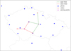 |
Fig. 1 Map of the Czech Republic showing the EN stations as blue diamonds, the stations with video cameras (red crosses), and the aiming points for the video experiments as magenta stars. |
2.2 Data processing
Each of the experiments employed in this campaign has its own way of data processing. For details, we refer to the papers mentioned above. Generally, following the observations, each data set was searched for the meteors. Detected meteors were catalogued, and their lists were compiled to obtain a global view of the recorded data and to be able to identify double or multi-station events. These meteors were manually measured using the FishScan software (Borovička et al. 2022b), and their atmospheric trajectories and heliocentric orbits were computed with the Boltrack program using standard procedures (Borovička et al. 2022b). For the single-station meteors, a shower membership was estimated based on their movement direction and angular velocity.
For meteors with known atmospheric trajectories, it is possible to measure the absolute brightness at each point. Firstly, the calibration curve is constructed based on the measured stars with known brightness. Then, the measured signal of the meteor is transformed into the apparent brightness using this curve. Finally, this value is recomputed on the distance of 100 km to obtain the absolute brightness. The photometric mass is computed using standard procedures (Ceplecha 1987). The luminous efficiency according to Pecina & Ceplecha (1983) was used to integrate the meteor light curve of the video meteors, whereas the method of ReVelle & Ceplecha (2001) was applied on the photographic records. When the photometry of the photographic meteors could not be obtained because no dynamic data were available, the meteor photometry was determined from IP cameras. The IP cameras were photometrically calibrated using photographic meteors, where the photometry was determined from DAFO by our standard procedures.
Only meteors with complete or almost complete light curves were used, that is, with a whole recorded luminous trajectory. Altogether, we counted 80 double or multi-station meteors, 23 of which were recorded by the DMK cameras, 34 by the Maia cameras, and 23 by the photographic cameras. An additional 55 single-station video meteors were used to compute the mass distribution index.
3 Meteor shower activity
The weather forecast was fulfilled quite well. Although the observational conditions were not ideal for some parts of the night because it was overcast, especially at the beginning of the observational window at some of the stations, the experiment was finally carried out successfully. The decision to stay within the fireball network and not to travel abroad was right. The fireball network cameras were operational for the whole night of 30/31 May from dusk to dawn. The video experiment was planned from 20 to 1:30 UT. It started later in the south due to cloudy sky, but after 22:30 UT, all the cameras were recording under an almost clear sky.
The shower membership was determined using the DSH criterion (Southworth & Hawkins 1963). As the reference orbits, the catalogue and the parent comet5 orbits (solution K222/29 for the 2017 apparition of the comets) were used. The meteors with DSH < 0.2 were accepted as τ Herculids. The trajectories of the single-station meteors were calculated under the assumption that they belong to the meteor shower, and if the radiant was found within 5 degrees from the mean radiant (compact group; see Sect. 4), they were also counted as τ Herculids.
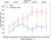 |
Fig. 2 Activity profile of the τ Herculid meteor shower. The red line represents a profile that is based on 207 meteors that were detected by all instruments and were counted in 30-min intervals. The profile based on the Ondřejov video camera data alone is drawn in blue. The edge intervals are not included because the data are incomplete (clouds at the beginning, and dawn at the end). |
3.1 Activity profile
To show the total activity profile, all the meteors identified as τ Herculids, the single- and double-station objects, that were detected by at least one of all used cameras were taken into account. We are aware that the numbers of meteors recorded by our cameras cannot be comparable with the numbers detected by the CAMS and GMN networks, but they still provide us with an insight into the activity level. Altogether, 207 τ Herculid meteors were counted in 30-min intervals, and these numbers were corrected for the zenith distance of the radiant. The resulting value was noted as the corrected hourly rate cHR, but this is not directly comparable with the zenith hourly rate that is traditionally used by visual observers. Because we observed only a few meteors, the shorter time intervals provide profiles that contain a number of fluctuations that may or may not be important.
According to the profile in Fig. 2, the activity started to increase after 21 UT and reached a relatively flat maximum around 23:30 UT. The activity varied between 70 and 80 meteors per hour for almost two hours. It began to decrease again after 1 UT, mainly due to the beginning of dawn.
As the video meteors dominate the τ Herculid meteor sample and two of four video cameras were disabled due to cloudy sky before 23 UT, this profile (we call it a ‘total’ because all instruments are included) may be biassed. To eliminate this bias, we concentrated on the Ondřejov station data because the sky became clear much earlier there. Only τ Herculid meteors recorded by the DMK and Maia cameras located at this station were used to calculate the profile in the same way as the profile described above. The result is depicted by the blue line in Fig. 2.
The comparison shows that the maximum activity occurred earlier, between 22 and 23 UT. The apparent later increase in the activity in the ‘total’ graph was probably a consequence of the fact that more video cameras contributed the counts. Some fluctuations are recorded after 23:30 UT, but due to the low number of the meteors, it is difficult to determine whether they are significant. However, the relatively high activity continued until 1 UT. This result agrees better with the visual observation activity profile presented in Rendtel & Arlt (2022). Initially, this timing suggested that an encounter with older filaments from the end of the 19th century could be observed.
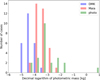 |
Fig. 3 Histogram of the photometric masses of meteoroids as recorded by different types of instruments. |
3.2 Mass distribution
Because different types of instruments were used, the range of photometric masses extends from 10−5 to about 10 kg. As expected, the faintest meteors (the lightest meteoroids) were recorded by DMK video cameras, and the brightest meteors (the heaviest) by the photographic cameras (Fig. 3).
As mentioned above, the already derived corrected hourly rate is instrument dependent and cannot be directly compared with similar quantities, either visual or instrumental. Therefore, it is necessary to convert the hourly rate into some universal quantity that does not depend on the instrument parameters. Such a quantity is the flux of the meteoroids. To be able to derive this, we need to determine the mass distribution index of the meteor shower. This is commonly measured as the linear part of the best fit of the log-log cumulative distribution (logarithm of mass vs. logarithm of the number of meteors). If the slope of the fit is k, then the mass distribution index s = 1 – k. If s < 2, then more mass is in larger particles, whereas s > 2 indicates that the stream contains many small particles (Blaauw et al. 2011).
The observations were carried out by two very different types of instruments. Firstly, the two double-station video experiments used cameras with a limited size of the field of view, and secondly, the photographic cameras of the fireball network are the all-sky cameras that are distributed in vast areas of central Europe (see Fig. 1). This means that the collection area of the two experiments cannot be compared. Biassed results of the mass distribution index would be obtained if all the masses of the observed meteors were taken into account. Moreover, the observation conditions changed at the beginning of the night, which is relatively simple to describe for the double-station experiment, but is more difficult for the all-sky cameras scattered around a larger area. For all these reasons, only video data were used to determine the mass distribution index. To correct for different collection areas, the numbers of the meteors detected by the DMK cameras were multiplied by the ratio of the collection areas of both instruments (which is approximately 8). The sample was extended by adding the singlestation meteors, for which the maximum apparent brightness was measured. Using the relation maximum apparent brightness versus photometric mass, which was found using the doublestation meteors, we estimated the photometric mass of the single station meteors.
The correction for different collection areas somewhat increased the number of meteors in the sample. Now, we worked with an equivalent of 675 meteors, which were arranged according to their photometric mass. The mean masses of groups containing 20 meteors are plotted in Fig. 4. The linear part of this plot was used to determine the mass distribution index, which is s = 2.02 ± 0.12. The corresponding value of the population index is r = 2.55.
Recently, a robust method for determining the mass distribution index was developed by Vida et al. (2020). It uses the maximum likelihood estimation (MLE) method to fit a gamma distribution to the observed distribution of masses. The source code is written in Python and is available in the Western Meteor Python Library6. The FitPopulationAndMassIndex.py software was applied to our data (corrected for the different collection areas of the cameras), and the resulting plot is shown in Fig. 5. This method provides the value s = 2.12 ± 0.07.
The visual observation data result in r = 2.40 ± 0.06 when the whole data set is used and r = 2.57 ± 0.23 when earlier activity alone is taken into account (Rendtel & Arlt 2022). The corresponding mass distribution indices are s = 1.98 and s = 2.03, respectively. The GMN preliminary report presents r = 2.5 ± 0.1 with a differential mass index s = 2.0 (Vida & Šegon 2022). Generally, all methods appear to result in a mass distribution index slightly higher than 2.
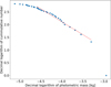 |
Fig. 4 Cumulative distribution of τ Herculid meteors recorded by the DMK and Maia cameras. The red line shows the fit of a linear part of the plot. The measured slope of the fit k = −1.02 is used to calculate the mass distribution index. Each point represents the mean value for 20 meteors. |
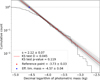 |
Fig. 5 Mass distribution index as computed by the software based on the MLE method (Vida et al. 2020). |
3.3 Meteoroid flux
To compute the meteoroid flux into the atmosphere, it is necessary to know the collection area of each camera. This was calculated according to the method presented by Brown et al. (2002b). This method neglects the Earth’s curvature as well as the certain decrease of the camera sensitivity towards the edge of the field of view. A height of the maximum brightness of the meteors HMAX = 88 km was used to determine the collection area (see Sect. 5.1). The meteoroid flux that produces meteors with a brightness up to the camera meteor limiting magnitude ΦMLM was computed as the corrected hourly rate (in 30-min intervals) divided by this collection area. Finally, this value is transformed into the flux of the meteoroids up to +6.5 mag Φ6.5 using the known values of the meteor limiting magnitude (MLM) of the camera and the population index (r) (Brown et al. 2002a),
 (1)
(1)
Because the sky was cloudy at Kunžak observatory at the beginning of the experiment, the flux was determined from the Ondřejov video data alone. The values used for the calculation are summarised in Table 1.
The flux of the meteoroids as recorded by the two video cameras at Ondřejov observatory is shown in Fig. 6. Although there are some fluctuations especially for the Maia camera, the values of the flux are relatively stable for several hours at around 0.0035±0.0013 meteoroids per km2 per hour up to the +6.5 mag. The fluctuations probably arise because only a small number of meteors was detected. A camera with a narrow field of view appears to be less sensitive to the fluctuations. The measured flux is approximately three times lower than the maximum flux reported by Vida & Šegon (2022) for the main peak of the shower activity. In comparison with other meteor shower outbursts, our measured value is about ten times lower than the maximum flux of the 2018 Draconids (Koten et al. 2020).
Parameters used to calculate the meteoroid flux.
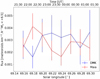 |
Fig. 6 Flux of the τ Herculid meteoroids. The flux is calculated as the corrected hourly rate per km2 per hour for meteoroids brighter than +6.5mag. The blue line represents the flux as recorded by the DMK camera, and the red line shows the flux as recorded by the Maia camera, both located at Ondrejov observatory. |
4 Radiants and orbits
Not many τ Herculid meteor orbits have been published so far. Some photographic results were reported by Southworth & Hawkins (1963) and Lindblad (1971). According to the IAU Meteor Data Center7, the radiant of the shower is αG = 228°.47, δG = 39°.91. This radiant was measured by Lindblad (1971). Hereafter, we refer to these coordinates as catalogue coordinates of the radiant. The predictions for the 2022 encounter differ from these values. They are summarised in Table 2.
We obtained a double- or multi-station solution for 80 τ Herculid meteors. The geocentric radiants of all meteors together with the positions of the modelled radiants are shown in Fig. 7. Two distinct areas can be seen here. Firstly, a relatively compact group of radiants is concentrated around αG = 209°.2, δG = 27°.9. Secondly, some radiants are scattered in the southwestern direction. The compact radiants are well consistent with the predictions of Horii et al. (2008) and Ye & Vaubaillon (2022).
The radiants are significantly shifted against the catalogue radiant. The angular distance of the centre of the compact area from the catalogue value mentioned above is about 20°. The distance of the scattered radiants is even higher. Only two meteors with radiants relatively close to the catalogue radiant were recorded. These meteors were not included in our data sample because they evidently do not belong to the analysed branch of the shower. As Fig. 7 also shows, the scattered radiants are not generally less precisely determined radiants. The size of the error bars is rather instrument dependent. The parameters of the photographic meteors are usually determined with lower errors than for the video meteors.
We compared the results with the known CAMS (Jenniskens 2022) and GMN (Vida & Šegon 2022) networks data. The measured radiants by both experiments are also listed in Table 2. For the CAMS data, the positions of the mean shower radiant are also provided for several days ahead of the maximum. On the other hand, the peak position for the GMN data is posted, as well as the average radiant shift. As Fig. 8 shows, the scattered radiants observed by our experiment are projected into the direction of the radiant shift. This might suggest that the meteoroid stream is wider and the particles are more scattered within it.
An explanation for the two groups of the radiants is provided by Egal et al. (2023). The compact area of the radiants is well consistent with the modelled radiants that originated from the 1995 comet break-up. On the other hand, the scattered radiants agree with the simulated meteoroids that were released between 1900 and 1947.
Several quantities were tested to determine whether they influence the position of the radiants in the plot. The photometric mass of the meteoroids, their semimajor axis, the perihelion distance, the time of their appearance expressed in terms of the solar longitude, the inclination of the orbit, and the DSH criterion were among the tested parameters. As an example, the distribution based on the DSH criterion against the 73P/Schwassmann-Wachmann 3 orbit is used in Fig. 9. The position of the radiant clearly does not depend on the distance between the comet and the meteoroid orbits. Moreover, this figure also shows that the heliocentric orbits of the majority of meteors are very close to the parent comet orbit with DSH < 0.06 (shades of blue).
No dependence on the majority of tested parameters was found. The only exception seems to be the inclination of the heliocentric orbit, as Fig. 10 suggests. There are meteors with a lower inclination among the scattered radiants, whereas the compact radiant area is dominated by the meteors with inclinations higher than 10.5°.
We compared the heliocentric orbits of both groups with the orbit of the parent comet. The results are shown in Table 3. With the exception of the argument of perihelion, the values of the compact group are slightly closer to the comet values. The higher inclination of the compact radiants is also seen from this table. The mean semimajor axis is slightly smaller than that of the parent comet for both groups of meteors. The histogram of the semimajor axis distribution is shown in Fig. 11. No dependence of the semimajor axis on the photometric mass was found.
Summary of the predicted and observed geocentric radiants for the 2022 τ Herculid meteor shower.
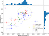 |
Fig. 7 Geocentric radiants of all observed τ Herculid meteors, regardless of the technique used. The radiant positions predicted by different models are also included. The dashed yellow circle represents a compact radiant area with a radius of 1.5°. |
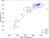 |
Fig. 8 Comparison of τ Herculid geocentric radiants observed by this experiment (blue circles), by the CAMS network (the red crosses represent the daily mean radiants), and the GMN network (the green circle represents the mean peak radiant). The CAMS daily mean positions are additionally annotated with the date (m = morning, and a = afternoon). The two positions without any annotation represent the evening and morning positions of the main peak night. Moreover, the radiant shift as recorded by the GMN is plotted for the last two days before the maximum (green dashed line). |
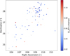 |
Fig. 9 Distribution of the geocentric radiants of τ Herculid meteors. The DSH criterion is colour-coded against the parent comet orbit. |
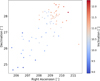 |
Fig. 10 Distribution of the geocentric radiants of τ Herculid meteors. The inclination of the heliocentric orbit is colour-coded. |
Heliocentric orbits of the two groups of τ Herculid meteors and the parent comet.
5 Physical properties
Our sample of τ Herculid meteors covers a range of the maximum brightness between 4.8 and −11.4 mag. The corresponding photometric masses range from 7.7 mg to about 10 kg, although the upper limit is probably even higher. This fact allowed us to investigate the properties of a broad range of meteoroid masses. The masses reach almost seven orders of magnitude.
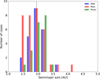 |
Fig. 11 Histogram of the semimajor axis distribution of τ Herculid meteors observed by different types of instruments. The mean value is marked by the dashed black line. |
5.1 Height data
The height data can be used as an insight into the meteoroid structure. Generally, three different types of instruments were used for the observation. Each of them is characterised by a different sensitivity. This means that the beginning heights of the photographic meteors, for instance, cannot be directly compared with the video meteors. Moreover, the two video experiments differ in their sensitivity. Therefore, the double-station meteors detected with the Maia cameras were selected for this analysis. They provide a slightly larger sample of uniform data than the DMK or photographic cameras.
The beginning height, the height of the maximum brightness, and the terminal height are plotted as a function of the photometric mass inFig. 12. The beginning heights are generally between 100 and 90 km. The beginning height increases with increasing photometric mass. The slope of the linear fit is about 3.9. This result agrees with the conclusion of Koten et al. (2004), who found that the beginning heights of cometary meteors increase with increasing photometric mass. On the other hand, when the slope of the fit is compared with the values presented in the mentioned paper for showers such as the Perseids, Taurids, and Orionids, the value found for τ Herculids is slightly lower. The dependence of the beginning height on the photometric mass is shallower than in other cometary meteor showers. On the other hand, it is still significantly higher than for the Geminid meteors, for which a completely different composition was found.
The height of the maximum brightness as well as the end height both decrease with increasing photometric mass. The linear fit for the latter is slightly steeper. This means that heavier meteoroids penetrate deeper into the atmosphere. The maximum brightness is usually between 90 and 85 km. The average value is HMAX = 88 km (the value used to calculate the collection area). The deepest penetration is about 80 km. The heights at which the τ Herculid meteors occurred are higher than expected for such slow meteors. When the observation campaign was planned, the aiming point for the double-station video observation was set at 80 km.
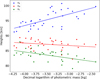 |
Fig. 12 Beginning height, height of the maximum brightness, and terminal height of the τ Herculid meteors detected by the Maia cameras. |
5.2 KB parameter and PE criterion
The altitude data are affected by the slope of the meteor trajectory and by the initial speed. Therefore, several dimensionless criteria were defined to compensate for these effects. A summary of them can be found in Ceplecha (1988). For faint television and video meteors, the KB parameter is used, which corrects the beginning height for the initial speed and slope of the tea-jectery. The meteoroids are classified into groups A, B, C, and D dependinm on trie KB value, eubgroups C1, C2, and C3 are defined according to the meteoroid orbit. The PE anh AL crileria are ueed for fireballs. Here, we applied the PE criterion, which compensates the terminal height for the meteoroid mass, initial speed, ang slope of the trajectory. A classification scheme consisting of groups I, II, IIIA, and IIIB was introduced according to this criterion.
Figure 13 shows the distribution of the KB parameter for theτ Herculidmeteors. The values range from 6.3 to 7.3, with a mean value  . Only ten meteors belong to group B, which represents dense cometary material. It is slightly surprising that this material is present within this cometary meteor shower. Therefore, records of these cases were checked again, and is was confirmed that the real beginning was measured for all of them. Most of the msteors fall into C group, which is regular cometary melerial. Wish a given semi-major axis and inclination, subgroup C1 contains τ Herculid meteors. Finally, a small portion of the meteors belongs to group D, representing soft cometary material.
We can compare the τ Herculie meteors with other meteor showers or sporadic meteors. Figure 13 also includes the KB parameters of the 2018 Draconids and of slow sporadics (υ∞, < 26 km s−1). Both sels of data were obtained with the same video system. The Draconids8 are usually thought to be very fragile meteoroids. (On the other hand, their speed (υ∞ ~ 23.6 km s−1) is higher than that of the τ Herculids (υ∞ ~ 16 km s−1 s−1). For lower masses down to 10 milligrams, their KB parameters are similar to those of the τ Herculid meteors. Generally, both shower mete-oroids are softer than the sporadic meteors and the velocity is similar because many sporadic meteors are of asteroidal origin.
Although the values of the KB criterion are scattered in a broad range for both meteor showers, there is a trend to lower values of the KB criterio n with increasing photometric mass. This trend is steeper for toe τ Herculid meteors. At lower masses, the Draconid meteoroids are softer, but at higher masses, the KB approach this value, and for the highest masses in the sample, they become very similar.
The classification of the τ Herculid photographic meteors according to the PE criterion is shown in Fig. 14, where different groups are also marked. Almost all meteors belong to IIIB (soft cometary material), and only Sew of them belong to group IIIA (regular cometary material). The trend in PE values depending on the mass of meteoroids is also very clear, that is, more massive meteoroids are more fregile. The PE criterion for 3 Draconid and other fireballs observed in 2017–2018 (Borovička et al. 2022a) shows that the τ Herculids we observed are the most fragile meteoroids observed ever. Their PE is usually lower than that of other meteors and even than that of Draconid meteors of the same mass.
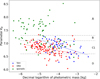 |
Fig. 13 KB parameter of τ Herculid, Draconid, and slow sporadic meteors (υ∞ < 20 km s−1) recorded by the same type of video camera, with limits for the classification scheme. The trends of KB for τ Herculids and Draconids are also shown. |
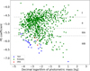 |
Fig. 14 PE criterioe of the τ Herculid photographic meteors (blue) and their comparison with Draconid (red) and other fireballs (green) from the catalogue of Borovička et al. (2022a). |
Atmospheric trajectory of the EN310522_013924 bolide.
5.3 EN310522_013924: The exceptional case of a bright τ Herculid bolide
Figure 14 shows a very bright and fragile bolide among the photographic meteors. This bolide was recorded by four all-sky photographic cameras and four IP video cameras at a total of six stations of the EN in the Czech Republic (3), Slovakia (2), and Austria (1) on 31 May 2023 at 1:39:22.5 ± 0.5 UT (for the bolide beginning). At this time, it was already late dawn, especially at the easternmost stations. As the bolide was flying over south-eastern Europe (Bosnia and Herzegovina), it was only detected at the southern EN stations, and it was very low above the horizon everywhere. Nevertheless, the high-quality and high-resolution recordings allowed us to determine all the parameters of its passage through the atmosphere with very good accuracy and reliability. The closest station (with a mean distance from the bolide of 465 km) from which we have both an all-sky photographic image and a video recording was Hur-banovo in southern Slovakia. The farthest station (mean distance 755 km) was Ondřejov (IP camera). The fact that the bolide was exceptionally bright is proved by the fact that it was well recorded at this large distance and also during dawn. This is confirmed by the analysis of the above records, from which we determined that the bolide reached a maximum absolute brightness of −11.6 mag and the initial meteoroid mass was 10 kg or slightly more. It should be emphasised here that the brightness and mass of the bolide were the most difficult of all parameters to determine, mainly because of the already very over-illuminated sky. It may therefore be affected by a somewhat larger error than all other parameters. It is also likely that the reported values of the brightness and mass are somewhat underestimated rather than unrealistically high.
The analysis of the physical properties of this meteoroid clearly shows that it was extremely fragile material. When we take the input mass mentioned above and the atmospheric trajectory parameters presented in Table 4 into account, the PE coefficient (Ceplecha 1988) describing the material properties of the body is −7.31. This value has not been observed for any other bolide in the entire existence of the EN. This indicates not only the extreme fragility of this meteoroid, but also its extremely low bulk density. For the most fragile meteoroids with a PE lower than −5.70, a bulk density of 270 kg m−3 (Ceplecha 1988) is usually given, but in this case, it must have been even much lower. Egal et al. (2023) modelled the light curves of two mete-oroids detected by CAMO and found bulk densities even lower, down to 230 kg m−3. However, even when we take a density of 270 kg m−3, the diameter of this meteoroid would be about 42 cm at the given mass. This is clearly only a lower estimate, and the real size of this meteoroid could easily have been about half a metre or even larger.
As explained above, unlike the brightness and mass, the trajectory is determined to a very good accuracy with a standard deviation of 65 metres for any point along the luminous path, and the initial velocity is determined even with a standard deviation of only 30 m s−1 (Table 5). A detailed analysis shows that the meteoroid entered the atmosphere at 16.0 km s−1 and started its light, that is, began to be visible for our cameras, at an altitude of 99.3 km. It travelled a 40.93 km long luminous trajectory in 2.55 s and terminated its flight at an altitude of 76.7 km. The entire atmospheric trajectory was over southeastern Bosnia and Herzegovina (east of Sarajevo). The data describing the atmospheric trajectory as well as its heliocentric orbit are given together with the corresponding standard deviations in Table 5. Similar to the atmospheric trajectory, the heliocentric orbit of this surprisingly large τ Herculid is determined reliably and matches the orbit of comet 73P/Schwassmann-Wachmann 3 very well. The similarity criterion DSH is only 0.023 (the cut-off value for DSH is = 0.20), and the other similarity criterion DD defined by Drummond (1981) is only 0.012 (the cut-off value for DD is = 0.105). Both values demonstrate a clear orbital connection between this meteoroid and the parent comet 73P/Schwassmann-Wachmann 3. Its radiant lies in the compact area.
The similarity of the orbit of such a massive and large meteoroid to the parent comet poses a significant challenge for modelling the evolution of this meteor shower. Most models mentioned above predicted that the particles released in 1995, which could reach the Earth’s orbit in 2022, could only be up to a millimetre in size. Egal et al. (2023) explained the observation of several bright fireballs using particles of a few centimetres that were released from the comet during the 1995 fragmentation event or during previous apparitions, but a half-metre size body still needs to be simulated. From this point of view, this is a very important observation that brings new and unexpected insights into the description of the dynamics of this meteor shower.
Radiants and orbital elements of the EN310522_013924 bolide (J2000.0).
5.4 Meteor spectra
Meteor spectra can be used to study the composition of mete-oroids and also their physical structure. The preferential release of sodium is a sign of early fragmentation into small grains (Borovička et al. 2014). The spectral video camera captured only two spectra of sufficient quality. The spectrum of meteor 22530019 (hereafter m019) was observed on the non-blazed side of the grating (–first order), which provides a much lower signal in the blue and green part of the spectrum. The spectrum of meteor 22530038 (hereafter m038) was observed in the +first order, but only until the wavelength of 610 nm. In addition, the spectrum of the terminal flare (magnitude −7.7) of the fireball EN300522_214616 (hereafter f214616) was obtained by an SDAFO. Some other spectra were obtained, but they show only the Na line. It is valid also for the spectrum of the very bright and distant fireball EN310522_013924 (see Sect. 5.3), which was captured by the IP camera in Kunžak.
The spectra of both video meteors evolved in time. At the beginning, only the Na line (589 nm) was present. Only when it became quite bright, did the lines of Fe and Mg at 510–550 nm and a continuum appear. The Na line then started to fade, while the Fe and Mg lines and the continuum kept their brightness. The continuum was especially well visible in m019 above 600 nm. The continuum showed no band structure, which means that it was a thermal continuum (with Planck temperature of about 2000 K) and not a molecular radiation, such as N2 or FeO observed in other meteors. While the Na line disappeared shortly before the meteor ended in m019, in m038, it retained some residual brightness. The other lines faded, and Na became the dominant spectral feature again, but at a lower intensity than at the beginning. Then, at the height of 84 km, a flare occurred. The Na line was very bright in the flare and remained visible also after the flare at lower heights. The spectra at different heights are plotted in Fig. 15. The spectrum of the flare is more noisy (especially around 450 nm) because it is a single-frame spectrum, while other spectra were averaged over several frames.
The photographic spectrum of f214616 was taken at a single height. Since the exposure was long, it contains both the spectrum of the fireball during the flare and the spectrum of a possible afterglow, which likely remained visible for some time at the same spot. Afterglows are typical by the presence of low excitation Fe lines (multiplets 1 and 2), and they are clearly seen in the spectrum. This spectrum has a higher resolution than the video spectra. It was possible to confirm that the Fe lines are brighter than the Mg lines at 516–519 nm. The brightest line was again the Na line, however.
Borovička et al. (2014) have shown on the example of the Draconids that meteoroids of the same stream that are observed in a single night can have different structure. Some meteoroids disintegrated into grains at the beginning of the trajectory, and some were more resistant. Since sodium easily evaporates from small grains, it appears and disappears earlier in the spectrum than other elements in the former case. Meteoroid m019 was such a case. Meteoroid m038 was a combined case. A larger part disintegrated at the beginning, at a height of about 96 km, and another part remained compact until a height of 84 km, where it erupted, and a small part continued at an even lower height.
When the line intensities are integrated along the whole trajectory, m038 can be classified as enhanced Na in the scheme of Borovička et al. (2005). In all τ Herculids with spectra, the Na line dominated and the Mg line was much fainter than in Draconids, for example. This fact can be partly connected with the lower velocity of τ Herculids. It is possible, however, that they were indeed richer in volatile sodium because they spent only 27 years in interplanetary space and were buried inside the comet before this.
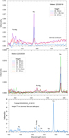 |
Fig. 15 Calibrated spectra of meteors 22530019 and 22530038 at various height ranges and the time-integrated spectrum of the fireball EN300522_214616 at the position of its terminal flare. The intensities are given in kW nm−1 ster−1. |
6 Discussion
A number of models predicted the possible activity of the τ Herculid meteor shower in the morning hours of 31 May 2022, caused by the material released from the parent comet during its 1995 outburst (for a summary, see Table 1 in Ye & Vaubaillon 2022). An earlier activity connected with this disruption event was not predicted. Only one older model by Wiegert et al. (2005) expected meteor shower activity before midnight, that is, in the very evening of 30 May. This activity should be connected with material released from the comet in 1892 and 1897.
Our video and photographic observations as well as the visual data of the IMO observers (Rendtel & Arlt 2022) and video data of the GMN (Vida & Šegon 2022) registered higher activity well above the annual level during the last hours of 30 May. When the model predictions are taken into account, this activity may be connected with 19th century perihelion passages of the parent comet. In terms of activity level, the event was weaker than other recent events, such as the modest outburst of the 2018 Draconid meteor shower. On the other hand, the activity was significant for the usually almost missing τ Herculid meteor shower and provided us with many valuable data.
An important contribution to the determination of the observed meteor origin was provided by the models of Egal et al. (2023). They simulated particles released from the parent comet at each apparition from 1800 as well as during the 1995 fragmentation of the comet. The modelled activity profile shows a secondary maximum between 15 and 19 UT on May 30 as well as the main peak after 4 UT on May 31. According to these models, our observation window fits between both peaks. The earlier peak was at its descending branch, whereas already ascending activity was connected with the main peak. The model also shows that the main peak was wider than originally expected. Therefore, we were able to record meteors belonging to the 1995 ejecta as well, although the observation period started hours before the predicted maximum.
The fact that we observed a mix of older meteoroids released before 1947 and young particles from the 1995 fragmentation is supported also by the comparison of the recorded and simulated radiants. Figure 16 shows that meteors recorded throughout the whole observation period contributed to both groups of radiants. The models of Egal et al. (2023) agree very well with our results. The scattered radiants are consistent with older meteoroids, and the compact radiants correspond to fresh meteoroids. The heliocentric orbits of most of the observed meteors are very close to the current orbit of the parent comet.
The analysis of the physical properties shows that the τ Herculid meteoroids are generally very fragile. Moreover, their fragility increases with increasing mass of the meteoroid. At the lowest masses, the particles appear to be slightly stronger than Draconid meteoroids. With increasing mass, the two groups of meteoroids become more similar. The trend of increasing fragility continues to higher masses. The τ Herculid meteors become, according to their PE criteria, even more fragile than the Draconids. When compared with other meteoroids of the same mass, their PE values are the lowest ever recorded.
The recorded spectra confirmed an early disruption of mete-oroids into grains, but also showed the existence of more resistant parts. A detailed meteoroid fragmentation modelling is planned for the future. The spectra also suggest an enhanced abundance of volatile sodium, which may be related to the short time the meteoroids were exposed to solar and cosmic radiation.
There are significant implications for the theoretical models of meteoroid stream formation and evolution. Much heavier particles than the models took into account were present. Initially, according to the models, only millimetre-size meteoroids were able to reach an Earth’s orbit. Already Ye & Vaubaillon (2022) noted that the observed meteoroids were heavier and hypothesised that the brighter meteors might be caused by centimetre-size porous dust aggregates. Egal et al. (2023) also took into account particles of a few centimetres. Particles much larger than centimetres were observed, however. The 10 kg meteoroid measured almost half a metre. This large body surely belongs to the 1995 fragmentation event. It is necessary to explain how these meteoroids could approach the Earth at the same time as the millimetre-size particles.
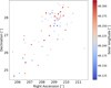 |
Fig. 16 Distribution of the geocentric radiants of the τ Herculid meteors. The solar longitude is colour-coded. The scattered and compact radiants are distributed throughout the whole observation period. |
Acknowledgements
This work was supported by the Grant Agency of the Czech Republic grants 20-10907S (video observation and analysis), 19-26232X (photographic observation and analysis) and the institutional project RVO:67985815 (institutional infrastructure). We thank the members of the Czech Hydrometeo-rological Institute for the forecast service in the days before the observations.
Appendix A Geocentric radiants and heliocentric orbits of the τ-Herculid meteors
Geocentric radiants of the τ Herculid meteors recorded by video cameras (J2000.0).
Heliocentric orbits of the τ Herculid meteors recorded by video cameras (J2000.0).
Geocentric radiants of the τ Herculid meteors recorded by photographic cameras (J2000.0).
Heliocentric orbits of the τ Herculid meteors recorded by photographic cameras (J2000.0).
References
- Blaauw, R. C., Campbell-Brown, M. D., & Weryk, R. J. 2011, MNRAS, 412, 2033 [NASA ADS] [CrossRef] [Google Scholar]
- Borovička, J., Koten, P., Spurný, P., Boček, J., & Štork, R. 2005, Icarus, 174, 15 [CrossRef] [Google Scholar]
- Borovička, J., Koten, P., Shrbený, L., Štork, R., & Hornoch, K. 2014, Earth Moon Planets, 113, 15 [CrossRef] [Google Scholar]
- Borovička, J., Spurný, P., & Shrbený, L. 2019, in International Meteor Conference, Pezinok-Modra, Slovakia, eds. R. Rudawska, J. Rendtel, C. Powell, et al., 28 [Google Scholar]
- Borovička, J., Spurný, P., & Shrbený, L. 2022a, A&A, 667, A158 [NASA ADS] [CrossRef] [EDP Sciences] [Google Scholar]
- Borovička, J., Spurný, P., Shrbený, L., et al. 2022b, A&A, 667, A157 [NASA ADS] [CrossRef] [EDP Sciences] [Google Scholar]
- Brown, P., Campbell, M., Suggs, R., et al. 2002a, MNRAS, 335, 473 [NASA ADS] [CrossRef] [Google Scholar]
- Brown, P., Campbell, M. D., Hawkes, R. L., Theijsmeijer, C., & Jones, J. 2002b, Planet. Space Sci., 50, 45 [NASA ADS] [CrossRef] [Google Scholar]
- Ceplecha, Z. 1987, Bull. Astron. Inst. Czechoslovakia, 38, 222 [NASA ADS] [Google Scholar]
- Ceplecha, Z. 1988, Bull. Astron. Inst. Czechoslovakia, 39, 221 [NASA ADS] [Google Scholar]
- Crovisier, J., Bockelee-Morvan, D., Gerard, E., et al. 1996, A&A, 310, L17 [NASA ADS] [Google Scholar]
- Drummond, J. D. 1981, Icarus, 45, 545 [NASA ADS] [CrossRef] [Google Scholar]
- Egal, A., Wiegert, P. A., Brown, P. G., & Vida, D. 2023, ApJ, 949, 96 [NASA ADS] [CrossRef] [Google Scholar]
- Horii, S., Watanabe, J.-I., & Sato, M. 2008, Earth Moon Planets, 102, 85 [NASA ADS] [CrossRef] [Google Scholar]
- Jenniskens, P. 2022, eMeteorNews, 7, 230 [NASA ADS] [Google Scholar]
- Koten, P., Borovička, J., Spurný, P., Betlem, H., & Evans, S. 2004, A&A, 428, 683 [NASA ADS] [CrossRef] [EDP Sciences] [Google Scholar]
- Koten, P., Fliegel, K., Vítek, S., & Páta, P. 2011, Earth Moon Planets, 108, 69 [NASA ADS] [CrossRef] [Google Scholar]
- Koten, P., Borovička, J., Vojáček, V., et al. 2020, Planet. Space Sci., 184, 104871 [NASA ADS] [CrossRef] [Google Scholar]
- Lindblad, B. A. 1971, Smith. Contrib. Astrophys., 12, 14 [NASA ADS] [CrossRef] [Google Scholar]
- Lüthen, H., Arlt, R., & Jäger, M. 2001, WGN J. Int. Meteor Organiz., 29, 15 [Google Scholar]
- Pecina, P., & Ceplecha, Z. 1983, Bull. Astron. Inst. Czechoslovakia, 34, 102 [NASA ADS] [Google Scholar]
- Rao, J. 2021, WGN J. Int. Meteor Organiz., 49, 3 [NASA ADS] [Google Scholar]
- Rendtel, J., & Arlt, R. 2022, WGN J. Int. Meteor Organization, 50, 92 [NASA ADS] [Google Scholar]
- ReVelle, D. O., & Ceplecha, Z. 2001, ESA SP, 495, 507 [NASA ADS] [Google Scholar]
- Shrbený, L., Spurný, P., & Borovička, J. 2020, Planet. Space Sci., 187, 104956 [CrossRef] [Google Scholar]
- Southworth, R. B., & Hawkins, G. S. 1963, Smith. Contrib. Astrophys., 7, 261 [NASA ADS] [Google Scholar]
- Spurný, P., Borovička, J., Mucke, H., & Svoreň, J. 2017, A&A, 605, A68 [NASA ADS] [CrossRef] [EDP Sciences] [Google Scholar]
- Vida, D., & Šegon, D. 2022, Central Bureau Electronic Telegrams, 5126, 1 [Google Scholar]
- Vida, D., Campbell-Brown, M., Brown, P. G., Egal, A., & Mazur, M. J. 2020, A&A, 635, A153 [NASA ADS] [CrossRef] [EDP Sciences] [Google Scholar]
- Wiegert, P. A., Brown, P. G., Vaubaillon, J., & Schijns, H. 2005, MNRAS, 361, 638 [NASA ADS] [CrossRef] [Google Scholar]
- Ye, Q., & Vaubaillon, J. 2022, MNRAS, 515, L45 [NASA ADS] [CrossRef] [Google Scholar]
061 TAH code in IAU MDC database.
009 DRA code in IAU MDC database.
All Tables
Summary of the predicted and observed geocentric radiants for the 2022 τ Herculid meteor shower.
Heliocentric orbits of the two groups of τ Herculid meteors and the parent comet.
Geocentric radiants of the τ Herculid meteors recorded by video cameras (J2000.0).
Heliocentric orbits of the τ Herculid meteors recorded by video cameras (J2000.0).
Geocentric radiants of the τ Herculid meteors recorded by photographic cameras (J2000.0).
Heliocentric orbits of the τ Herculid meteors recorded by photographic cameras (J2000.0).
All Figures
|
Fig. 1 Map of the Czech Republic showing the EN stations as blue diamonds, the stations with video cameras (red crosses), and the aiming points for the video experiments as magenta stars. |
| In the text | |
|
Fig. 2 Activity profile of the τ Herculid meteor shower. The red line represents a profile that is based on 207 meteors that were detected by all instruments and were counted in 30-min intervals. The profile based on the Ondřejov video camera data alone is drawn in blue. The edge intervals are not included because the data are incomplete (clouds at the beginning, and dawn at the end). |
| In the text | |
|
Fig. 3 Histogram of the photometric masses of meteoroids as recorded by different types of instruments. |
| In the text | |
|
Fig. 4 Cumulative distribution of τ Herculid meteors recorded by the DMK and Maia cameras. The red line shows the fit of a linear part of the plot. The measured slope of the fit k = −1.02 is used to calculate the mass distribution index. Each point represents the mean value for 20 meteors. |
| In the text | |
|
Fig. 5 Mass distribution index as computed by the software based on the MLE method (Vida et al. 2020). |
| In the text | |
|
Fig. 6 Flux of the τ Herculid meteoroids. The flux is calculated as the corrected hourly rate per km2 per hour for meteoroids brighter than +6.5mag. The blue line represents the flux as recorded by the DMK camera, and the red line shows the flux as recorded by the Maia camera, both located at Ondrejov observatory. |
| In the text | |
|
Fig. 7 Geocentric radiants of all observed τ Herculid meteors, regardless of the technique used. The radiant positions predicted by different models are also included. The dashed yellow circle represents a compact radiant area with a radius of 1.5°. |
| In the text | |
|
Fig. 8 Comparison of τ Herculid geocentric radiants observed by this experiment (blue circles), by the CAMS network (the red crosses represent the daily mean radiants), and the GMN network (the green circle represents the mean peak radiant). The CAMS daily mean positions are additionally annotated with the date (m = morning, and a = afternoon). The two positions without any annotation represent the evening and morning positions of the main peak night. Moreover, the radiant shift as recorded by the GMN is plotted for the last two days before the maximum (green dashed line). |
| In the text | |
|
Fig. 9 Distribution of the geocentric radiants of τ Herculid meteors. The DSH criterion is colour-coded against the parent comet orbit. |
| In the text | |
|
Fig. 10 Distribution of the geocentric radiants of τ Herculid meteors. The inclination of the heliocentric orbit is colour-coded. |
| In the text | |
|
Fig. 11 Histogram of the semimajor axis distribution of τ Herculid meteors observed by different types of instruments. The mean value is marked by the dashed black line. |
| In the text | |
|
Fig. 12 Beginning height, height of the maximum brightness, and terminal height of the τ Herculid meteors detected by the Maia cameras. |
| In the text | |
|
Fig. 13 KB parameter of τ Herculid, Draconid, and slow sporadic meteors (υ∞ < 20 km s−1) recorded by the same type of video camera, with limits for the classification scheme. The trends of KB for τ Herculids and Draconids are also shown. |
| In the text | |
|
Fig. 14 PE criterioe of the τ Herculid photographic meteors (blue) and their comparison with Draconid (red) and other fireballs (green) from the catalogue of Borovička et al. (2022a). |
| In the text | |
|
Fig. 15 Calibrated spectra of meteors 22530019 and 22530038 at various height ranges and the time-integrated spectrum of the fireball EN300522_214616 at the position of its terminal flare. The intensities are given in kW nm−1 ster−1. |
| In the text | |
|
Fig. 16 Distribution of the geocentric radiants of the τ Herculid meteors. The solar longitude is colour-coded. The scattered and compact radiants are distributed throughout the whole observation period. |
| In the text | |
Current usage metrics show cumulative count of Article Views (full-text article views including HTML views, PDF and ePub downloads, according to the available data) and Abstracts Views on Vision4Press platform.
Data correspond to usage on the plateform after 2015. The current usage metrics is available 48-96 hours after online publication and is updated daily on week days.
Initial download of the metrics may take a while.