| Issue |
A&A
Volume 675, July 2023
|
|
|---|---|---|
| Article Number | A45 | |
| Number of page(s) | 8 | |
| Section | The Sun and the Heliosphere | |
| DOI | https://doi.org/10.1051/0004-6361/202346089 | |
| Published online | 30 June 2023 | |
The He I 10 830 Å line: Radiative transfer and differential illumination effects
1
Instituto de Astrofísica de Canarias, 38205 La Laguna, Tenerife, Spain
e-mail: This email address is being protected from spambots. You need JavaScript enabled to view it.
2
Departamento de Astrofísica, Universidad de La Laguna, 38206 La Laguna, Tenerife, Spain
3
Astronomical Institute of the Academy of Sciences, Fričova 298, 251 65 Ondřejov, Czech Republic
Received:
6
February
2023
Accepted:
14
May
2023
Abstract
We study the formation of the Stokes profiles of the He I multiplet at 10 830 Å when relaxing two of the approximations that are typically considered in the modeling of this multiplet. Specifically, these are the lack of self-consistent radiation transfer and the assumption of equal illumination of the individual multiplet components. This He I multiplet is among the most important for the diagnostics of the outer solar atmosphere from spectropolarimetric observations, especially in prominences, filaments, and spicules. However, the aptness of these approximations is yet to be assessed, especially in situations where the optical thickness is on the order of one (or greater) and the radiation transfer has a significant impact in the local anisotropy as well as the ensuing spectral line polarization. This issue becomes particularly relevant in the ongoing development of new inversion tools that take into account multi-dimensional radiation transfer effects. To relax these approximations, we generalized the multi-term equations for the atomic statistical equilibrium to allow for a differential illumination of the multiplet components and implement them in a one-dimensional (1D) radiative transfer code. We find that even for this simple geometry and relatively small optical thickness, both radiation transfer and differential illumination effects have a significant impact on the emergent polarization profiles. These effects should be taken into account in order to avoid potentially significant errors when inferring the magnetic field vector.
Key words: atomic processes / polarization / radiative transfer / Sun: atmosphere
© The Authors 2023
 Open Access article, published by EDP Sciences, under the terms of the Creative Commons Attribution License (https://creativecommons.org/licenses/by/4.0), which permits unrestricted use, distribution, and reproduction in any medium, provided the original work is properly cited.
This article is published in open access under the Subscribe to Open model. This email address is being protected from spambots. You need JavaScript enabled to view it. to support open access publication.
1. Introduction
The magnetic field is fundamental to our understanding of commonly observed plasma structures such as prominences, filaments, and spicules, as it is responsible for their structures, properties, and even their very existence (see, e.g., reviews in Mackay et al. 2010 and Tsiropoula et al. 2012). Spectropolarimetric observations of the He I multiplets at 10 830 Å (hereafter, 10 830 multiplet) and 5876 Å (usually dubbed D3) have been extensively acquired and analyzed to diagnose these structures and, in particular, to infer their magnetic fields (see and references therein Trujillo Bueno & del Pino Alemán 2022).
The formation of the Stokes profiles of these ortohelium spectral lines is somewhat difficult to model due to their sensitivity to the coronal UV/FUV illumination (Judge & Centeno 2008), which ionizes the neutral helium atoms that can then be recombined to populate the relatively high-excitation energy triplet states. However, this property is what has also allowed for the modeling of these lines to be significantly simplified. It turns out that the 10 830 multiplet and D3 cannot effectively form in quiet Sun conditions, as it is only observable in magnetically active regions and in plasma structures such as prominences, filaments, and spicules. Because they form in more or less localized plasma regions with a somewhat small optical thickness, it is generally assumed that it is possible to model these multiplets with a relatively simple slab model, without accounting for radiation transfer (RT) effects and with the most complex processes (e.g., coronal illumination) abstracted into the optical thickness of the slab. This fact has been exploited in the HAZEL inversion code (Asensio Ramos et al. 2008), which has been widely used for the analysis of spectropolarimetric observations in prominences, filaments, and spicules (see the review Trujillo Bueno & del Pino Alemán 2022 and references therein).
Apart from this apparent simplicity in their modeling, the 10 830 and D3 multiplets are both fully observable with today’s instrumentation and their spectral line polarization is sensitive to the magnetic field with strengths between a fraction of a gauss to a few hundred gauss – values that are expected to be typical for structures of the outer atmosphere. Moreover, their polarization is sensitive to the magnetic field via the Hanle and Zeeman effects, and elastic collisions with neutral hydrogen atoms in chromospheric and prominence plasma are unlikely to significantly reduce the atomic polarization of the He I levels (Sahal-Bréchot et al. 1977; Casini et al. 2009)1. All of these facts taken together have made these He I multiplets incredibly useful in the context of inferring the magnetic field vector in the above-mentioned regions of the solar atmosphere.
The formation of the Stokes profiles of the 10830 and D3 multiplets can be described with the quantum theory of atomic line formation (Landi Degl’Innocenti & Landolfi 2004). In particular, the multi-term model atom is the most suitable for this application (see Sects. 7.5, 7.6, and 13.4 of Landi Degl’Innocenti & Landolfi 2004 for a detailed description of the problem). One important requirement for the applicability of the multi-term model atom is that the exciting radiation field must be spectrally flat2 over the wavelength range spanned by the multiplet components. For the 10 830 multiplet this implies that the blue and red components (remembering that the red component is a blend of two of the lines of this triplet), which are about 1 Å apart, must be excited by identical radiation fields (and likewise for D3 and its components).
This assumption is very well satisfied if the optical thickness of the multiplet components is small (τ < 1) and the exciting illumination is that of the relatively flat continuum of the quiet photosphere. However, observations clearly indicate that the optical thickness of the 10 830 multiplet can often exceed one (e.g., Díaz Baso et al. 2019a,b). For plasmas that are optically thick enough, RT effects within the region of formation of the He I multiplets lead to a spectrally non-flat radiation field. Due to the non-negligible separation in wavelength between the red and blue components of the 10 830 multiplet, and the difference of their optical thicknesses, the radiation field becomes indeed non-flat and the multi-term model atom equations are no longer suitable. Even though the potential importance of these RT effects in the 10 830 multiplet have been recognized before (see Trujillo Bueno & Asensio Ramos 2007), no detailed investigation of this problem has ever been conducted.
The so-called flat-spectrum condition or approximation is due to the fact that the theory of complete frequency redistribution (CRD, LL04 is based on the first-order perturbative expansion of the matter–radiation interaction. In order to relax this condition, it is necessary to use a higher order theory, which would allow us to consider coherent scattering processes and partial frequency redistribution (PRD) effects (Stenflo 1994; Bommier 1997a,b, 2017; Casini et al. 2014). However, including PRD effects dramatically increases the computing time requirements, which prevents it for being considered a particularly desirable approach for a multiplet that can otherwise be successfully modeled by assuming complete frequency redistribution (Asensio Ramos et al. 2008). Assuming a multi-level model atom (see Sects. 7.1 and 7.2 of Landi Degl’Innocenti & Landolfi 2004) also naturally relaxes this assumption. However, the quantum interference between the upper levels of the blended red components of the 10 830 multiplet needs to be taken into account to correctly model their polarization, which is not possible within this model.
In this paper, we propose a new approach to the 10 830 multiplet formation that is more general than the multi-term model atom – at least for the magnetic fields strengths relevant for chromospheric and coronal spectropolarimetry. Our formulation allows us to treat separately the illumination of the red and blue components of the 10 830 multiplet. The multi-term model atom is the limit case of our method, which is strictly valid in the case of spectrally flat illumination and negligible optical thickness of the medium. In contrast to the multi-term approximation, our approach allows us to solve the problems out of the local thermodynamic equilibrium approximation (NLTE) in plasmas of any optical thickness. As we show below, this approach leads to significant modification of the traditional results in 1D slab models. Moreover, NLTE RT plays an even more important role in the formation of the lines of the outer solar atmosphere if 3D effects are considered (Štěpán et al. 2022).
In order to be able to consider NLTE models involving the 10 830 line, we need to realize that the quantum interference between the upper level of the blue component and the other two levels in the term is not expected to have a significant impact for the typical magnetic fields found in the solar atmosphere. We thus derived a new set of statistical equilibrium equations (SEE) starting from the multi-term model atom of Landi Degl’Innocenti & Landolfi (2004) and explicitly removing the quantum interference between the upper level of the blue component and the rest of the levels. This allows us to introduce different pumping radiation fields for the blue and red components of the 10 830 multiplet. We implemented this new set of equations into a 1D RT code.
In Sect. 2, we describe the new set of SEE and some details about the RT code. In Sect. 3, we carry out a series of numerical experiments to study the impact of RT and differential illumination effects on the emergent Stokes profiles. Finally, we present our conclusions in Sect. 4.
2. Formulation of the problem
The theory of atomic line polarization, summarized in the monograph by Landi Degl’Innocenti & Landolfi (2004), is formulated in the frame of the so-called complete frequency redistribution (CRD). This limit of atom-photon interactions, which implies a complete lack of correlation between the frequencies of the absorbed and emitted photons in scattering processes, has been immensely useful in inferring magnetic fields of the solar atmosphere during the last decades.
The multi-term model atom, described in Chapter 7 of Landi Degl’Innocenti & Landolfi (2004) is the most suitable to describe the 10 830 multiplet as it accounts for quantum interference between states |βLSJM⟩ and |βLSJ′M′⟩ of different J and J′ levels of the same βLS term. However, in order to ensure physical consistency when accounting for quantum interference between non-degenerate atomic levels, the incident radiation field must have a flat spectrum across a frequency range wider than the separation of those levels. In addition, the CRD theory is strictly valid if the incident radiation field is flat on a frequency interval much larger than the natural width of the atomic states. Due to the small natural width of the 10 830 multiplet sublevels, this condition is automatically satisfied if the spectrum is flat across the whole multiplet.
When these conditions are satisfied, the absorption and stimulated emission within a spectral line depend on the frequency independent radiation field tensor:
 (1)
(1)
where ϕ(ν) is the normalized line’s absorption profile, and  is the radiation field tensor at each frequency ν. We note that the ϕ(ν) absorption profile is representative of the absorption in the whole multiplet and thus it has the shape of the absorptivity, and not that of a Voigt profile. Strictly speaking, this approach is only valid if all the multiplet components have comparable absorptivities and are illuminated by similar enough radiation fields, which is not necessarily true for the 10 830 multiplet.
It is then clear that if we want to introduce different radiation fields for the blue and red components in the SEE, we need to neglect quantum interference between the blue component’s upper level and any of the red component’s upper levels. Consequently, only the two red component’s upper levels can be coherent. In this way, we can still fulfill the validity condition of the CRD approximation, that is, spectral flatness on a frequency interval much larger than the natural width of each transition, as well as the validity condition of the multi-term atom model, namely, spectral flatness in a frequency range wider than the separation between levels that can be coherent.
Generally, the further in energy two levels, the less significant the quantum interference between them. The separation between the J = 0 state, the upper level of the blue component of the 10 830 multiplet, from the rest of the states is about 30 GHz (or 0.1 meV) that is, about four orders of magnitude larger than the natural width of the Zeeman states, which is about 1.6 MHz or 10−5 meV. This energy separation remains very large even if the magnetic states are modified by a magnetic field with strength up to ∼5 kG, when some of the Zeeman components of the upper levels of the red component crosses with the blue component’s upper level (see Fig. 1). Therefore, for the typical magnetic fields found in the solar atmosphere, we can safely neglect quantum interference between the upper levels of the blue and red components, and, thus, we can consider different radiation fields for each component, while ensuring that the CRD theory remains strictly valid.
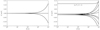 |
Fig. 1. Energy of the magnetic sublevels of the lower (left panel) and upper (right panel) terms of the 10 830 Å multiplet as a function of the magnetic field strength. The natural widths of the upper-term levels is about 10−5 meV, which is well below the plotting resolution. The zero energy offsets in each panel correspond to the mean energies of the respective terms. |
Consequently, the only difference with respect to the standard multi-term SEE (see Sect. 7.6 in Landi Degl’Innocenti & Landolfi 2004) is that instead of considering a single radiation field for the whole multiplet, we distinguish between the radiation field in the red and blue components, forcing the quantum interference between magnetic states pertaining to different components to vanish. Therefore, instead of a single  radiation tensor common to all the multiplet sublevels, we now have
  or
or  , resulting from the same average as in Eq. (1), but integrating over ϕ(ν)red and ϕ(ν)blue. The absorption profiles only account for the contributions for the red or the blue component, respectively. In our approach, we follow the standard way of derivation of the equations and we diagonalize the atomic Hamiltonian in the incomplete Paschen-Back effect regime. Consequently, the RT coefficients in the RT equation have exactly the same formal expression as the corresponding coefficients of Landi Degl’Innocenti & Landolfi (2004). These relatively minor changes in the SEE allow us to consider a much broader set of physical scenarios. We implemented these SEE in a 1D RT code, which solves the NLTE problem of the generation and transfer of polarized radiation.
3. Numerical experiments
In this section, we show the result of some numerical experiments to illustrate how accounting for differential radiation between the red and blue components of the 10 830 multiplet, as well as RT effects, can lead to strikingly different emergent Stokes profiles.
We compare the results obtained with our code with those obtained under the assumption of flat-spectrum and negligible impact of the RT effects on the atomic density matrix. For this physical scenario, the RT equations have the solution (see, e.g., Asensio Ramos et al. 2008):
![Mathematical equation: $$ \begin{aligned} \boldsymbol{I} = \left[\boldsymbol{1} + \psi _{\rm O} \boldsymbol{K}\prime \right]^{-1} \left[ (\mathrm{e} ^{-\tau }\mathbf 1 - \psi _{\rm M}\boldsymbol{K}\prime )\boldsymbol{I}_{\rm inc} + (\psi _{\rm M} + \psi _{\rm O})\boldsymbol{S} \right], \end{aligned} $$](/articles/aa/full_html/2023/07/aa46089-23/aa46089-23-eq6.gif) (2)
(2)
where 1 is the unit matrix, K′=K/ηI − 1, with K the propagation matrix and ηI the absorption coefficient for intensity, S is the source function vector, and Iinc is the Stokes vector of the incident radiation (at the lower boundary of the slab). The coefficients ψO and ψM only depend on the optical depth along the propagation direction at a particular frequency and angle, and their expression can be found in Kunasz & Auer (1988). Due to its simplicity and straightforward evaluation, the linear Eq. (2) is commonly used in practical applications to invert spectropolarimetric data of the 10 830 multiplet.
As noted above, Eq. (2) is applicable if both K′ and S are constant along the ray of propagation. This is a good approximation if the optical thickness is below unity. We note that while this approximation does include radiation transfer via Eq. (2), it is not self-consistent, as the radiation field is assumed fixed and constant throughout the whole extension of the slab. However, for greater optical thicknesses, this approximation becomes unsuitable because RT starts playing a significant role (see Trujillo Bueno & Asensio Ramos 2007). The problem then becomes non-local and non-linear. The notably different opacities between the red and blue components also lead to the non-fulfillment of the spectral flatness approximation.
Equation (2) is strictly valid for an optically thin slab illuminated with a spectrally flat incident radiation. We have checked that, in this limit, our calculations coincide with the result of Eq. (2) for magnetic fields from zero to several thousands of gauss (see Sect. 3.2).
3.1. Impact on the radiation field anisotropy
In this experiment, we considered a slab with constant properties located 6 Mm above the solar surface, with its normal axis parallel to the solar radius. The optical thickness of the slab was τ = 2 in the center of the red component of the 10 830 multiplet. We solved the self-consistent RT transfer problem in this slab model.
In this first experiment, we assumed that the slab is unmagnetized (B = 0) and we analyze the wavelength variation of the  and
and  (mean intensity and anisotropy, respectively) components of the radiation field tensor at different optical depths from the top, τ = 0, to the bottom, τ = 2, boundaries (see Fig. 2). In Eq. (2), the radiation field tensor is constant throughout the slab and spectrally flat (red dashed line, hereafter, the non-RT model). However, the radiation field tensor components in the self-consistent solution (solid curves, hereafter RT model) show a strong dependence on height due to the combination of RT effects and the differential absorption and emission in the red and blue components of the multiplet.
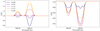 |
Fig. 2. Mean intensity ( |


At the top of the slab (τ = 0, dark blue curve), the mean intensity spectrum (left panel of Fig. 2) resembles the typical 10 830 absorption profiles. This can easily be understood primarily in terms of the absorption of the incident intensity in the slab’s bottom boundary. At the bottom of the slab (τ = 2, yellow curve), however, the mean intensity shows an excess with respect to the mean intensity of the incident continuum radiation. This is due to the radiation that is emitted from within the slab and traveling “downward”.
Regarding the radiation field anisotropy (right panel of Fig. 2), we see a reduction with respect to the incident anisotropy, a reduction which is non-monotonic with the optical depth. This reduction is mainly a consequence of the horizontal RT within the slab: for inclined lines of sight, there is a larger amount of emitting material, which increases the negative contribution of the radiation coming from directions forming an angle with the slab’s axis that is larger than the van Vleck angle (see, e.g., Trujillo Bueno 2001). For this reason, the largest differences between the non-RT and RT model’s anisotropies are found at optical depths around τ = 1, where the radiation is more likely to start escaping the slab along the vertical direction, while the more inclined rays are still optically thick.
From this experiment, it is clear that RT and the relaxation of the flat spectrum approximation can have a considerable impact on the radiation field tensors that (as we show in subsequent experiments) can significantly impact the emergent Stokes parameters.
3.2. Impact on the emergent Stokes profiles
Even with a relatively small optical thickness of τ = 2, NLTE RT effects significantly modify the radiation field anisotropy within the slab. Since this quantity is crucial for the emitted linear scattering polarization, we can expect RT effects to have a significant impact on the emergent Stokes profiles as well.
We considered the same physical scenario as in Sect. 3.1, but with a uniform and horizontal (perpendicular to the slab’s axis) magnetic field of B = 10 G. After solving the self-consistent NLTE problem, we calculated the emergent Stokes profiles for a line of sight parallel to the slab’s axis. We note that if the slab and the incident illumination at the bottom boundary are axially symmetric, as it would be the case if it was not for the chosen magnetic field, there would be no polarization when observing along the slab’s axis due to the symmetry. Thus, the magnetic field is necessary to generate scattering linear polarization via the Hanle effect in the chosen model and line of sight. This would correspond, for example, to the observation of a filament close to the disk-center. By choosing the reference direction for the linear polarization parallel to the magnetic field vector, the only non-zero Stokes parameters are I and Q.
In Fig. 3, we show the emergent Stokes profiles for three cases: (i) the non-RT model (orange solid curve), (ii) the RT model with the flat spectrum across the whole multiplet approximation (dashed blue curve, hereafter RT-flat model), and (iii) the RT model (solid blue curve).
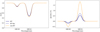 |
Fig. 3. Intensity I (left panel) and Q (right panel) line profiles normalized to the continuum intensity for both the constant-property slab model solution (orange) and fully consistent NLTE solution (blue) for disk-center observation of the τ = 2 slab with horizontal magnetic filed with B = 10 G. The positive Q direction is parallel to the projection of the magnetic field vector onto the plane of the sky. |
Regarding the intensity (left panel of Fig. 3), the impact of the approximations is relatively minor. Assuming (or not) a flat spectrum across the whole multiplet does not have a significant impact if one solves the self-consistent problem, and fully neglecting RT effects only has some impact on the depth of the red component. This difference could lead to a slight error on the determination of the optical thicknesses or the Doppler width (equivalently, the temperature) of the slab, but we do not expect such a difference to be significant.
One interesting aspect to note is what happens to the polarization (right panel of Fig. 3). The flat spectrum approximation in the self-consistent (RT-flat model) solution results in a significant increase of the emergent linear polarization, changing the ratio between the polarization signals of the blue and red components. Moreover, if RT is also neglected (non-RT model), the calculated emergent linear polarization is even larger, resulting in an increase by more than a factor of three with respect to the RT model.
Consequently, both RT effects and the flat-spectrum approximation have a significant impact on the linear polarization profiles. This difference in the signal is directly related to the changes in the frequency-independent anisotropy, as defined in Eq. (1), with the suitable absorption profiles. In particular, the anisotropy in the red component, which determines the alignment of the red component’s upper levels, is smaller in the RT model than in the non-RT model in the whole slab; it is also smaller than the anisotropy of the RT-flat model in the upper part of the slab (τ ≤ 1) where most of the photons emerge from. Curiously, the anisotropy of the blue component is significantly larger than that of the RT-flat model and of the red component in the RT model (although it is still smaller than the anisotropy in the non-RT model). However, the blue component’s upper level is non-polarizable (J = 0) and thus the polarization of this line is fully due to dichroism; namely, it is due to the atomic alignment of the lower level (Trujillo Bueno et al. 2002). It turns out that the impact of the red component on the lower level alignment is characterized as being smaller when we relax the flat spectrum approximation and so, the emergent linear polarization in the RT model is consistently smaller across the whole multiplet.
We can further study the impact of these approximations by comparing the fractional linear polarization signal at the peaks of the blue and red components for different magnetic field strengths and for several optical thicknesses (see Fig. 4). For the chosen model (disk-center line of sight, axially symmetric slab model), the horizontal magnetic field breaks the axial symmetry and induces linear polarization. Up to a few gauss, in the Hanle regime, the polarization increases with the magnetic field. For larger magnetic field strengths, the Hanle effect is in saturation and the linear polarization is insensitive to changes in the magnetic field strength (plateau in the linear polarization in Fig. 4). For magnetic field strengths in the hundreds, the Zeeman effect starts affecting the linear polarization, as seen at the end of the plateau toward the largest field strengths in Fig. 4. For small optical thicknesses (e.g., τ = 0.01, the optically thin limit; see top-left panel of Fig. 4), the three approaches produce (as expected) the same polarization signal for every magnetic field. However, for increasingly larger optical thicknesses, RT effects induce a significant reduction of the anisotropy and thus of the polarization signal, which is more significant the larger is the optical thickness. This behavior will saturate when the optical thickness is large enough as to thermalize the bottom boundary of the slab. The relaxation of the flat-spectrum approximation also has an impact on the emergent linear polarization signals (compare the solid and dashed curves in Fig. 3), but the most significant reduction in the polarization emergent from the slab is due to RT effects (compare the dashed and dotted curves in the figure).
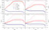 |
Fig. 4. Fractional linear polarization, Q/I, as a function of magnetic field strength for different optical thicknesses specified at the top-left of each panel. The blue (red) curves correspond to the blue (red) component of the 10 830 multiplet. The dotted curve shows the result with the non-RT model, the dashed curve shows the result with the RT-flat model, and the solid curve shows the result with the RT model. Note: the vertical-axis scale is different in each panel. |
In summary, in this particular model, the NLTE solution leads to a significant decrease in the anisotropy within the slab and to a decrease in the 10 830 polarization amplitude. Consequently, the interpretation of the observations based on the optically thin slab model with the flat-spectrum approximation, the non-RT model could lead to significant errors in the determination of the slab’s physical properties, especially with respect to the magnetic field vector. This error can be critical depending on the particular physical scenario: assuming an observation of a solar filament with a horizontal magnetic field in the Hanle saturation regime (e.g., 20 gauss), for which we are able to delimit its height (if not, we would face a different problem with respect to an almost complete degeneration between height and magnetic field strength as inversion parameters). The non-RT model would overestimate the anisotropy and the inversion algorithm would need to pick a magnetic field strength in the Hanle regime, where the linear polarization is still sensitive to the magnetic field strength, in order to find a smaller polarization signal that fits the observation for the overestimated anisotropy. We would then infer magnetic field strengths in the fractions of gauss (𝒪(10−1)), instead of a magnetic field in the saturation regime (𝒪(101–102)). The opposite would happen in the prominence scenario, where a horizontal field depolarizes the zero-field scattering signal. In order to compensate for the excess in anisotropy from the non-RT assumption, the inferred magnetic field is increased, which could lead to the identification of field strengths of fractions of gauss (𝒪(10−1)) as magnetic fields in the saturation regime (𝒪(101–102)). We emphasize, however, that a non-RT model would also be unable to correctly fit the linear polarization profiles altogether. In the non-RT model, the ratio between the amplitudes of the red and blue components is fixed for each value of the signal of any of the two components. Because the ratio between these two signals with RT is different, there is no combination of parameters (in a constant property slab) for which the emergent Stokes parameters from Eq. (2) would adequately fit the RT profiles.
Although our conclusions are not model-dependent3, their quantification indeed is. While the non-RT slab model shows these issues are due to the non-RT assumption, the RT slab model finds itself in the opposite extreme, that is, where the optical thickness tends to infinity in the horizontal direction. We must thus emphasize that while our modeling exposes a potential problem in the inference of magnetic fields with the non-RT model, what we show in this paper is the worst case scenario. First, the reduction of the anisotropy calculated in the slab is an upper limit. Secondly, the observation of circular polarization can alleviate the problem by providing a constraint in the magnetic field longitudinal component (we have intentionally chosen a physical scenario without circular polarization in this paper), even though this cannot fully solve issues related to the direction of the magnetic field vector and it can even make it impossible to fit the four Stokes parameters simultaneously.
These findings are consistent with what was found in the observation and analysis of the 10 830 multiplet in prominences and filaments. In general terms, as explained above, it may explain why prominences seem to show magnetic fields in the saturation regime, while quiet Sun filaments seem to show magnetic fields in the fractions or units of gauss, namely, in the Hanle regime (see Trujillo Bueno & del Pino Alemán 2022 and references therein). Regarding the particular case of filaments, there are (as far as we know) only a few filament observations with the dichroic blue component signal, and the inversion is usually unable to achieve a completely satisfactory fit. Trujillo Bueno et al. (2002) showed a fit to a filament profile, demonstrating the dichroic origin of the blue component’s linear polarizaiton signal; however, their fit does not match the blue component’s intensity (see their Fig. 4). Lagg et al. (2004) showed a fit to a profile in a flux emergence region, neglecting lower level polarization, that is unable to fit the blue component’s linear polarization (see their Figs. 4 and 5). Later, Asensio Ramos et al. (2008) showed a fit to the same profiles including lower level polarization and, while it is improved, they were unable to simultaneously fit the linear polarization amplitude of both the blue and red components (see their Fig. 16, as well as Fig. 14 for an example with other filament observations). Díaz Baso et al. (2019a,b) found and studied this impossibility in the fitting, even though their observations show peculiar polarization signals with the same sign in both red and blue components, which require additional complexity in the physical model beyond RT4. Other filament observations include those of Kuckein et al. (2012) and Xu et al. (2012), who found mostly Zeeman linear polarization profiles in filaments on top of active regions and thus could be fit (see Figs. 7–9 in Kuckein et al. 2012 and Fig. 4 in Xu et al. 2012). Curiously, Kuckein et al. (2009) posit that a reduction factor of 0.2 was needed in the anisotropy in order to explain their filament observations, a similar reduction to the one we find in our model for the red component’s anisotropy at τ = 1 (∼0.17, see Fig. 2). All in all, observations of filaments in the 10 830 multiplet are relatively scarce, but they tend to show that the non-RT model may not be enough to find a satisfactory fit to the observed linear polarization profiles (see Fig. 4). Consequently, in order to correctly interpret observations in filaments with a relatively large optical thickness, we think that RT must be taken into account, the flat spectrum approximation must be relaxed, and that a model more complex than a constant property slab is necessary to explain observations, such as those of Díaz Baso et al. (2019a,b).
4. Conclusions
We have investigated the impact of RT effects on the polarization of the 10 830 multiplet. In particular, we have studied the effect that relaxing the flat spectrum approximation (requiring us to consider that both components are illuminated by identical radiation fields) has on the anisotropy and on the emergent linear scattering polarization. To this end, we have modified the SEE for the multi-term atom, neglecting quantum interference terms between the blue component’s upper level and the two red component’s upper levels. Moreover, instead of calculating a singular average radiation field for the whole multiplet (Eq. (1)), we computed the equivalent quantity for each of the components, where the absorption profile is constructed by including only contributions to the absorptivity from magnetic line components pertaining to each of the blue or red components of the 10 830 multiplet. We implemented this modified set of equations into a 1D RT code and calculated the 10 830 multiplet emergent Stokes profiles in a constant property slab model in order to compare our results with those obtained with the usual modeling assumptions of these lines, namely, no RT and flat-spectrum across the whole multiplet (non-RT model).
In the optical thin limit, our self-consistent calculations coincide with those of the non-RT model, as expected. As we increase the optical thickness of the slab, the results start to diverge and for an optical thickness that is not too large, we start to observe significant differences among the results. First, allowing for RT within the slab significantly affects the radiation field. The mean intensity in the top (bottom) region of the slab shows a significant defect (excess) in the lines due to the absorption (emission) by the rest of the slab below (above). The radiation field anisotropy is instead diminished with respect to the non-RT case due to the significant contribution of the radiation propagating along the more inclined directions, which are optically thicker due to the geometry, as anticipated by Trujillo Bueno & Asensio Ramos (2007).
More important, especially for the diagnostic of the magnetic field, are the differences in the emergent Stokes profiles. For a slab of an optical thickness τ = 2, we only find a small difference in the red component’s intensity, which could slightly impact the determination of the optical thickness and temperature (via the Doppler width). However, the difference is remarkable for the linear scattering polarization, on the order of a factor three in the signal of both components. Due to the larger anisotropy in the non-RT model, which is diminished when horizontal RT within the slab is accounted for, the linear polarization is significantly overestimated. This can undoubtedly lead to an underestimation of the magnetic field or the filament height for this particular disk-center filament configuration. This would result in a difference that is potentially of a few orders of magnitude in the magnetic field strength in the worst-case scenarios. In fact, filament observations showing scattering polarization signals in the blue component, as far as we know, cannot be usually completely fit for both the blue and red components. Moreover, some observations show signals with the same sign in both the blue and red components – something that we have not achieved in reproducing for a constant property slab even with RT. This could mean that the constant property slab model (both RT and non-RT) is too simplistic to model these observations.
The impact of the RT will be even more significant in full 3D geometry (e.g., Štěpán & Trujillo Bueno 2013). First, a non-homogeneous volume of plasma with enough optical thickness will not only reduce the anisotropy of the incoming radiation from the underlying disk, but also contribute to the breaking of axial symmetry, an additional source of linear polarization, which can only be accounted for by the magnetic field in the commonly used slab model. Secondly, recent 3D NLTE RT calculations in an academic two-level atom model indicate that already for optical thicknesses as small as τ = 1, RT plays an important role in spectral line formation (see Fig. 9 of Štěpán et al. 2022).
Last but not least, we note that another important multiplet of He I, namely, the D3 multiplet at 5876 Å, is most likely optically thin in all the structures of the outer solar atmosphere and, therefore, it is less prone to be impacted by the effects discussed in this paper. However, since the lower term of D3 is the upper term of 10 830, both multiplets are coupled. An investigation of the impact of the 10 830 transfer on the D3 line remains one of our research topics for the near future.
The results presented in this paper expose a potential problem of the simplified non-RT modeling of such complex structures. While its simplifications allow for the implementation of extremely fast inversion codes, we need to be careful when the plasma conditions do not allow for the simplifications to be truly fulfilled. This emphasizes the relevance of developing novel diagnostic techniques that can account for important physical ingredients such as the full three-dimensional geometry and RT effects. For this reason, we are developing an inversion code based on the ideas presented in Štěpán et al. (2022), and we will continue the investigation started in this paper with significantly more generality (with 3D RT) in a forthcoming publication.
As far as we are aware, the role of depolarizing collisions in the ortohelium levels has not been studied in great detail in the literature, although they may possibly play a role in sufficiently dense active region filaments.
The Stokes parameters are constant with wavelength.
The very same argument can be made just by knowing that RT effects reduce the anisotropy, a fact that has been known for decades (Trujillo Bueno & Asensio Ramos 2007).
We have not been able to find emergent Stokes profiles with the same sign signals with our code in a constant property slab, except for particular combinations of magnetic fields and velocities resulting in amplitudes much smaller than those observed.
Acknowledgments
We are grateful to Luca Belluzzi, Javier Trujillo Bueno, and Andrés Asensio Ramos for number of suggestions that helped us to improve the paper. We acknowledge the funding received from the European Research Council (ERC) under the European Union’s Horizon 2020 research and innovation program (ERC Advanced Grant agreement No 742265). J.Š. acknowledges the financial support of the grant 19-20632S of the Czech Grant Foundation (GAČR) and the support from project RVO:67985815 of the Astronomical Institute of the Czech Academy of Sciences. T.P.A.’s participation in the publication is part of the Project RYC2021-034006-I, funded by MICIN/AEI/10.13039/501100011033, and the European Union “NextGenerationEU”/RTRP. M.J.M.G.’s participation in this research has been supported by the project PGC-2018-102108-B-100 of the Spanish Ministry of Science and Innovation and by the financial support through the Ramón y Cajal fellowship. We also acknowledge the community effort devoted to the development of the following open-source packages that were used in this work: numpy (https://numpy.org/, Harris et al. 2020, matplotlib (https://matplotlib.org/, Hunter 2007). We made the code publicly available in a github repository https://github.com/andreuva/He1083RT.
References
- Asensio Ramos, A., Trujillo Bueno, J., & Landi Degl’Innocenti, E. 2008, ApJ, 683, 542 [Google Scholar]
- Bommier, V. 1997a, A&A, 328, 706 [NASA ADS] [Google Scholar]
- Bommier, V. 1997b, A&A, 328, 726 [NASA ADS] [Google Scholar]
- Bommier, V. 2017, A&A, 607, A50 [NASA ADS] [CrossRef] [EDP Sciences] [Google Scholar]
- Casini, R., Manso Sainz, R., & Low, B. C. 2009, ApJ, 701, L43 [NASA ADS] [CrossRef] [Google Scholar]
- Casini, R., Landi Degl’Innocenti, M., Manso Sainz, R., Landi Degl’Innocenti, E., & Landolfi, M. 2014, ApJ, 791, 94 [NASA ADS] [CrossRef] [Google Scholar]
- Díaz Baso, C. J., Martínez González, M. J., & Asensio Ramos, A. 2019a, A&A, 625, A128 [NASA ADS] [CrossRef] [EDP Sciences] [Google Scholar]
- Díaz Baso, C. J., Martínez González, M. J., & Asensio Ramos, A. 2019b, A&A, 625, A129 [NASA ADS] [CrossRef] [EDP Sciences] [Google Scholar]
- Harris, C. R., Millman, K. J., van der Walt, S. J., et al. 2020, Nature, 585, 357 [NASA ADS] [CrossRef] [Google Scholar]
- Hunter, J. D. 2007, Comput. Sci. Eng., 9, 90 [NASA ADS] [CrossRef] [Google Scholar]
- Judge, P., & Centeno, R. 2008, ApJ, 687, 1388 [NASA ADS] [CrossRef] [Google Scholar]
- Kuckein, C., Centeno, R., Martínez Pillet, V., et al. 2009, A&A, 501, 1113 [NASA ADS] [CrossRef] [EDP Sciences] [Google Scholar]
- Kuckein, C., Martínez Pillet, V., & Centeno, R. 2012, A&A, 539, A131 [NASA ADS] [CrossRef] [EDP Sciences] [Google Scholar]
- Kunasz, P., & Auer, L. H. 1988, J. Quant. Spec. Radiat. Transf., 39, 67 [NASA ADS] [CrossRef] [Google Scholar]
- Lagg, A., Woch, J., Krupp, N., & Solanki, S. K. 2004, A&A, 414, 1109 [NASA ADS] [CrossRef] [EDP Sciences] [Google Scholar]
- Landi Degl’Innocenti, E., & Landolfi, M. 2004, Polarization in Spectral Lines (Kluwer Academic Publishers, Dordrecht), 307 [Google Scholar]
- Mackay, D. H., Karpen, J. T., Ballester, J. L., Schmieder, B., & Aulanier, G. 2010, Space Sci. Rev., 151, 333 [Google Scholar]
- Sahal-Bréchot, S., Bommier, V., & Leroy, J. L. 1977, A&A, 59, 223 [Google Scholar]
- Stenflo, J. 1994, Solar Magnetic Fields: Polarized Radiation Diagnostics (Berlin: Springer), 189, 385 [NASA ADS] [Google Scholar]
- Trujillo Bueno, J. 2001, ASP Conf. Ser., 236, 161 [Google Scholar]
- Trujillo Bueno, J., & Asensio Ramos, A. 2007, ApJ, 655, 642 [NASA ADS] [CrossRef] [Google Scholar]
- Trujillo Bueno, J., & del Pino Alemán, T. 2022, ARA&A, 60, 415 [NASA ADS] [CrossRef] [Google Scholar]
- Trujillo Bueno, J., Landi Degl’Innocenti, E., Collados, M., Merenda, L., & Manso Sainz, R. 2002, Nature, 415, 403 [Google Scholar]
- Tsiropoula, G., Tziotziou, K., Kontogiannis, I., et al. 2012, Space Sci. Rev., 169, 181 [Google Scholar]
- Štěpán, J., & Trujillo Bueno, J. 2013, A&A, 557, A143 [NASA ADS] [CrossRef] [EDP Sciences] [Google Scholar]
- Štěpán, J., del Pino Alemán, T., & Trujillo Bueno, J. 2022, A&A, 659, A137 [NASA ADS] [CrossRef] [EDP Sciences] [Google Scholar]
- Xu, Z., Lagg, A., Solanki, S., & Liu, Y. 2012, ApJ, 749, 138 [Google Scholar]
All Figures
|
Fig. 1. Energy of the magnetic sublevels of the lower (left panel) and upper (right panel) terms of the 10 830 Å multiplet as a function of the magnetic field strength. The natural widths of the upper-term levels is about 10−5 meV, which is well below the plotting resolution. The zero energy offsets in each panel correspond to the mean energies of the respective terms. |
| In the text | |
|
Fig. 2. Mean intensity ( |
| In the text | |
|
Fig. 3. Intensity I (left panel) and Q (right panel) line profiles normalized to the continuum intensity for both the constant-property slab model solution (orange) and fully consistent NLTE solution (blue) for disk-center observation of the τ = 2 slab with horizontal magnetic filed with B = 10 G. The positive Q direction is parallel to the projection of the magnetic field vector onto the plane of the sky. |
| In the text | |
|
Fig. 4. Fractional linear polarization, Q/I, as a function of magnetic field strength for different optical thicknesses specified at the top-left of each panel. The blue (red) curves correspond to the blue (red) component of the 10 830 multiplet. The dotted curve shows the result with the non-RT model, the dashed curve shows the result with the RT-flat model, and the solid curve shows the result with the RT model. Note: the vertical-axis scale is different in each panel. |
| In the text | |
Current usage metrics show cumulative count of Article Views (full-text article views including HTML views, PDF and ePub downloads, according to the available data) and Abstracts Views on Vision4Press platform.
Data correspond to usage on the plateform after 2015. The current usage metrics is available 48-96 hours after online publication and is updated daily on week days.
Initial download of the metrics may take a while.