| Issue |
A&A
Volume 674, June 2023
|
|
|---|---|---|
| Article Number | A78 | |
| Number of page(s) | 7 | |
| Section | Galactic structure, stellar clusters and populations | |
| DOI | https://doi.org/10.1051/0004-6361/202346249 | |
| Published online | 06 June 2023 | |
Evidence of a common origin for the Virgo overdensity and Hercules-Aquila Cloud from abundances and orbital parameters
1
Shandong Provincial Key Laboratory of Optical Astronomy and Solar-Terrestrial Environment, School of Space Science and Physics, Shandong University at Weihai, Weihai 264209, PR China
e-mail: This email address is being protected from spambots. You need JavaScript enabled to view it.
2
CAS Key Laboratory of Optical Astronomy, National Astronomical Observatories, Chinese Academy of Sciences, Beijing 100101, PR China
3
School of Astronomy and Space Science, University of Chinese Academy of Sciences, Beijing 100049, PR China
Received:
26
February
2023
Accepted:
23
April
2023
Abstract
Aims. The Virgo overdensity (VOD) and the Hercules-Aquila cloud (HAC) may have originated from the same accretion event. In this work, we use K giants from the Large Sky Area Multi-Object Fiber Spectroscopic Telescope (LAMOST) survey to further investigate their potentially common origins.
Methods. We selected member stars in the VOD and HAC regions from the K giant sample of LAMOST DR5 and cross-matched them with results from the literature to obtain their elemental abundances. The orbital characteristics, namely, eccentricity, apocenter distance, energy, and angular momentum were compared between the member stars in the VOD and HAC regions. Then, we investigated the relationship between the VOD and HAC from the perspective of chemical evolution through a comparison of the distributions of elemental abundances in these two regions.
Results. By studying the orbital parameters of the members in VOD and HAC, we find that the distribution of the orbital eccentricity, apocenter, and maximum height from the Galactic disk of the members of these two regions are very consistent. They are both on orbits of low angular momentum and high energy. Their density distributions in the spatial position are also similar based on an integration of the last 8 Gyr of their orbits. We also found that these two structures have similar distributions in [Fe/H] and other elemental abundances. Based on the similarity of the orbital properties and the consistency of the chemical abundances, we suggest that these two structures may have come from the merger of the same dwarf galaxy, such as the Gaia-Sausage-Enceladus (GSE). Also, part of the VOD may originate from Small Magellanic Cloud (SMC) debris that had been stripped 3 Gyr ago.
Key words: Galaxy: structure / stars: abundances
© The Authors 2023
 Open Access article, published by EDP Sciences, under the terms of the Creative Commons Attribution License (https://creativecommons.org/licenses/by/4.0), which permits unrestricted use, distribution, and reproduction in any medium, provided the original work is properly cited.
This article is published in open access under the Subscribe to Open model. This email address is being protected from spambots. You need JavaScript enabled to view it. to support open access publication.
1. Introduction
The formation and evolution of galaxies is one of the most important field of modern astrophysics and the study of galaxy formation has made great progress in recent years. The power spectrum of density fluctuations measured by Wilkinson Microwave Anisotropy Probe (WMAP) is in good agreement with ΛCDM (Searle & Zinn 1978; Spergel et al. 2003; Bullock & Johnston 2005), which has made the hierarchical model of galaxy formation more widely accepted. Models of hierarchical structure formation predict that such galaxies as the Milky Way are formed by a series of accretion and merger events, in which smaller galaxies form larger ones via accretion or mergers. With the wide-field photometric surveys, such as Sloan Digital Sky Survey (SDSS; York et al. 2000), and Two Micron All-Sky Survey (2MASS; Skrutskie et al. 2006), numerous streams and overdensities have been discovered in the past two decades. The most prominent stellar streams are the Sagittarius tidal streams (Ivezić et al. 2000; Yanny et al. 2000; Vivas et al. 2001; Majewski et al. 2003; Shi et al. 2012; Zhang et al. 2017) and the Monoceros stellar stream (Newberg et al. 2002; Rocha-Pinto et al. 2003). In addition, there are many smaller streams and abundant dwarf galaxies in the so-called field of streams (Belokurov et al. 2006). The origins of some substructures are not well understood and they may be shown to be the result of multiple processes. In this work, we concentrate on two cloud-like overdensities: the Virgo overdensity (VOD) and Hercules-Aquila cloud (HAC).
Using RR Lyrae stars from the Quasar Equatorial Survey Team survey, the VOD was first identified by Vivas et al. (2001). Shortly thereafter, Newberg et al. (2002) also found an overdensity region using F-type turnoff starcounts on the celestial equator in approximately the same region of the sky, which they called S297+63-20.0. Jurić et al. (2008) identified a halo structure covering more than 1000 deg2 of the sky in the north Galactic cap using SDSS. The halo structure named VOD is at a distance of 6–20 kpc from the Sun. Carlin et al. (2012) found a similar orbit using 16 stars with measured proper motions that were plausibly part of Virgo stellar stream (VSS). Evidence has been building to indicate that both the VOD and VSS could have originated from a single merger event on a highly eccentric orbit. However, Duffau et al. (2014) and Vivas et al. (2016) found several halo substructures along the same line of sight in VOD. Zinn et al. (2014) and Donlon et al. (2019) regarded a large number of identified moving groups as evidence that the structures might not actually share a common origin after all.
The HAC region is an overdense region discovered by Belokurov et al. (2007) using main sequence turnoff stars. It is located at l (25°∼ − 60°), b (−40°∼ 40°) and is at a distance of 10–20 kpc from the Sun (Belokurov et al. 2007; Simion et al. 2014).
Simion et al. (2019) used a sample of ∼350 RR Lyrae stars with radial velocities and proper motions (Gaia Data Release 2) to study the orbital properties of the VOD and HAC. These authors concluded, based on an orbital integration, that VOD and HAC are actually debris from the remnants of an identical merger event. Han et al. (2022) suggested that VOD and HAC are long-lived structures associated with Gaia-Sausage-Enceladus (GSE) and that the dark matter halo of the Galaxy is tilted with respect to the disk and aligned in the direction of VOD-HAC. Perottoni et al. (2022) combined data from Sloan Extension for Galactic Understanding and Exploration (SEGUE), Apache Point Observatory Galactic Evolution Experiment (APOGEE) and Gaia to investigate the three structures from the orbit and chemistry, concluding that VOD and HAC are from the GSE merger.
In this paper, we use the member stars of VOD and HAC selected by Yang et al. (2019) in combination with information of element abundances from Xiang et al. (2019) to study the connection of orbital properties and chemical origin between VOD and HAC.
This paper is organized as follows. In Sect. 2, we present the data selection and the dynamical properties of VOD and HAC regions. In Sect. 3, we investigate the distribution of elemental abundances in VOD and HAC regions. A brief discussion and summary are given in Sects. 4 and 5.
2. Data and kinematic properties
2.1. The sample and its spatial and velocity distributions
Yang et al. (2019) selected the member stars of VOD (106 stars) and HAC (56 stars) from the sample of K giants from Large Sky Area Multi-Object Fiber Spectroscopic Telescope (LAMOST; Cui et al. 2012; Zhao et al. 2006, 2012) DR5 by the friend-of-friend (fof) algorithm. We used the sample of member stars provided in that sample, combined with the elemental abundance information provided by Xiang et al. (2019) to analyze the properties of VOD and HAC.
Figure 1 illustrates the distribution of the spatial positions of the member stars in the VOD and HAC regions. We used a left-handed coordinate system with the Galactic center as the coordinate origin. The Sun is located at the Galactic center (X, Y, Z) = (−8.3 kpc, 0 kpc, 0 kpc). The X-axis points positively to the Galactic center and Z-axis points to the north Galactic pole. The left panel shows the distribution of the member stars in the Galactic coordinate system, while the middle and right panels show the distribution of the member stars in X–Y and X–Z, respectively.
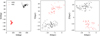 |
Fig. 1. Distributions of the two fields (VOD and HAC) in the (l, b), (X–Y), (X–Z) space. Black dots: member stars of VOD. Red dots: member stars of HAC. |
From the spatial distribution of these two structures, we can see that these two structures are at a long distance from one another. In the distribution of the Galactic coordinate system (left panel of Fig. 1), VOD is in the high-latitude region and HAC is in the low-latitude region. The reason for the relative spatial distribution of these two structures could be generated by the serial impacts caused by the GSE merger event (Iorio & Belokurov 2019).
Figure 2 shows the velocity distribution in a spherical coordinate system. For the calculation of the velocity distribution in the spherical coordinate system, we use the astropy package (Astropy Collaboration 2018) and correct the solar reflex motion (U, V, W) = (11.1, 12.4, 7.25) km s−1 (Schönrich et al. 2010) and circular velocity (220 km s−1) at solar radius for the solar motion (Bovy 2015). The diagrams show the three-dimensional (3D) velocity distribution of the member stars in the VOD and HAC regions. Vr, Vϕ, Vθ represent the radial velocity, azimuthal velocity, and polar velocity, respectively.
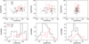 |
Fig. 2. Velocity distribution in spherical polar coordinates (Vr, Vϕ, and Vθ are the radial, azimuthal, and polar components, in km s−1) of the VOD and HAC. Upper panels: scatter diagrams of the velocity distributions of the VOD (black) and HAC (red). Lower panels: histograms displaying the velocity distributions of VOD (black) and HAC (red) members. |
We take the absolute values of the velocities in three directions and calculate their mean and variance, as shown in Table 1. Based on the mean and variance we find that the mean values of their velocity distributions in three directions are similar. The dispersions are also quite similar.
Mean and standard deviation of the velocity components.
Comparing the space and the velocity distributions, we find that the two structures are long-distance in spatial position but are mixed well in velocity space. This indicates that the two structures show similar characteristics in the velocity distribution.
2.2. Orbital parameters
To further understand the relationship between VOD and HAC, we investigated the kinematic nature of the two regions. We computed the orbits of the member stars of the VOD and HAC regions using the galpy package1 (Bovy 2015). We initialized the orbits with the covariance under the Galactic-centered column coordinate system, used the gravitational potential model of MWPOTENTIAL2014, and calculated the eccentricity of the orbits, the apocenter and pericenter points, and the maximum height from the Galactic Plane (Zmax). Figure 3 plots the distribution of the orbital eccentricity and Zmax, the apocenter point and the Galactic center distance. In the lower panels, “pdf” indicates the percentage distribution function. From the distribution of the orbits, we can find that the orbital eccentricities of the VOD and HAC are highly consistent, which are basically greater than 0.7. This indicates that both regions are in high eccentricity orbits, which is consistent with the conclusion of Simion et al. (2019). In the distribution of Zmax, though a little part of the HAC region is below 10 kpc, but for Zmax larger than 10 kpc, the Zmax distributions of VOD and HAC overlap each other. From middle panels of Fig. 3, we find that the apocenter points of VOD and HAC are mainly concentrated around 15–30 kpc. Both of these regions are also concentrated around 10–20 kpc from the galactic center. We performed the Kolmogorov-Smirnoff (K-S) test on the orbital eccentricities of the two regions, and obtained the P-value of 0.98. Thus, we can accept with high confidence that the orbital eccentricities of the member stars in the two regions obey a similar distribution pattern. It is possible that they have the same origin from the orbital parameters.
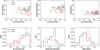 |
Fig. 3. Properties of the stellar orbits in the VOD and HAC fields. Upper panels: maximal height above the galactic plane, apocentre, and Galactocentric radius as a function of eccentricity, for the VOD (black) and HAC (red) stars. Lower panels: histogram distribution of eccentricity, apocentre, and Galactocentric distance. |
2.3. Energy and angular momentum distribution
The energy and angular momentum distributions can also give an indication of the relationship between different substructures in the Galaxy, so we plotted the energy and angular momentum distributions in both VOD and HAC regions, as in Fig. 4. In the left panel of Fig. 4, we show the distribution of L⊥ (Vertical component of angular momentum) and Lz (z-component of angular momentum) in these two regions. The right panel shows the distribution of angular momentum and energy. We can clearly find that these two structures also overlap each other in energy and angular momentum space, and both are in high-energy and low-angular-momentum orbits. Donlon et al. (2019) suggested the dwarf galaxy passed very close to the Galactic center and the debris has a large range of energies but nearly zero Lz angular momentum. In this work, the distribution of angular momentum and energies of both VOD and HAC are consistent with the view of Donlon et al. (2019). Although VOD and HAC are at a long distance in terms of position, the distribution of angular momentum further indicates that their movement trends are similar.
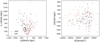 |
Fig. 4. Distribution of the angular momentum and the energy in the VOD (black dots) and HAC (red dots) regions. |
2.4. Orbital distribution of VOD and HAC
The orbits may provide another piece of evidence supporting the correlations between VOD and HAC. We calculated the past 8 Gyr orbits of the VOD and HAC regions based on the initialization of the components under the galactic column coordinate system. We plot the density distribution of the orbits over past 8 Gyr in Fig. 5. From the figure, we can find that the density distributions of these two regions are very similar. In the Galaxy coordinate system, VOD spans a somewhat wider latitude than that of HAC, which may be due to the fact that the VOD region is broader than the HAC region. For the distributions on X–Z, both regions show an X-shaped distribution in the Z-direction, intersecting at the center. According to the distributions of the spatial locations of VOD and HAC, VOD has a higher distribution in the Z-direction, with its X–Z distribution (shown in Fig. 5) shown to be a little more elongated than that of HAC, with a extension of 20 kpc. The similarity of the density distribution is consistent with the results of Simion et al. (2019) and Simion et al. (2018).
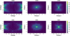 |
Fig. 5. Density maps of the member stars along their individual orbits over the past 8 Gyr, in Galactic coordinates (left panels) and in the X–Y (middle) and Y–Z (right). |
3. Element abundance distributions of VOD and HAC
As shown in Sect. 2, from a kinematic point of view, these two structures are somewhat related and may come from the same merger event. To better support the validity of our idea, we explored the connection between the two regions through the elemental abundances. Xiang et al. (2019) present the determination of stellar parameters and individual elemental abundances for 6 million stars from about 8 million low-resolution (R ∼ 1800) spectra from LAMOST DR5. By cross-matching with the data of Xiang et al. (2019), we obtained information on the elemental abundances of the members of the VOD and HAC regions. The histograms of various elemental abundances are shown in Fig. 6. The solid black line indicates the elemental abundance distribution of the member stars in the VOD region and the red dashed line indicates the elemental abundance distribution of the member stars in the HAC region. We can see that the distributions of [Fe/H], [C/Fe], [Ca/Fe], and [Ti/Fe] are very similar in both regions, with common peaks. For [O/Fe] and [Si/Fe] there are small deviations, probably due to the selection effect of the data. The similar distribution of element abundances further suggests that the two structures may be from the same merger event. Figure 7 illustrates the distribution of element abundances with [Fe/H] and Vr with [Fe/H]. The black dots indicate the VOD member stars, and the red dots indicate the HAC member stars. We find that the elements abundance in these two regions is mixed very well, further suggesting that they may have a common evolutionary origin. The lower-right panel in Fig. 7 shows the distribution of the radial velocity with [Fe/H], and we can find that the element abundances of VOD and HAC regions are similar, although one is moving toward us and the other is moving away from us.
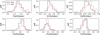 |
Fig. 6. Histogram distribution of elements abundance. Solid black line indicates VOD members and the red dashed line indicates HAC members. |
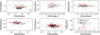 |
Fig. 7. Distribution of element abundances with [Fe/H] and the distribution of the radial velocity with [Fe/H]. |
To test our hypothesis that these two regions have the similar elemental abundances distribution, we selected the elemental abundances [Fe/H], [Ca/Fe], and [Ti/Fe] and calculated the p-values for their K-S tests. Based on the histogram of the elemental distribution (Fig. 6), we see that there are some extreme distributions that will cause inaccuracy in our test for the overall sample. So we first calculated the mean μ and standard deviation σ of these three abundances, and then selected data in the range of μ + 3σ and μ − 3σ for the K-S test. The results of the K-S test were: P[Fe/H] = 1.00, P[Ca/Fe] = 0.99, P[Ti/Fe] = 1.00. From the distribution of element abundances, we cannot distinguish them from each other, indicating that they may have a common origin in chemical evolution, which is similar to the view of Perottoni et al. (2022).
4. Discussion the origin
The origins of VOD and HAC may be rooted in other other events, aside from the GSE merger mentioned above. Li et al. (2016) used the data from the first year of Dark Energy Survey (DES) to find a stellar overdensity region named EriPhe at (l ∼ 285°, b ∼ −60°) and suggested that there is a possibility that this structure is part of the polar orbit structure formed by EriPhe, VOD, and HAC stellar overdensities. The locations of EriPhe, VOD, and HAC is shown in Fig. 8. Arrows indicate the velocity direction and the length of arrows show the size of velocity. The reverse extension line of arrows of VOD and HAC cross at a point, which is near the Galactic center. We speculate that there may have been an explosion or a splash event (Belokurov et al. 2020) that took place some many Gyr ago, which caused VOD, HAC, and EriPhe to move to their present position. EriPhe can not be observed with LAMOST, but with the advent of China Space Station Telescope (CSST), this structure can be explored with deep space observations. Thus, we will be able to further investigate the relationship of the three structures and verify our speculations.
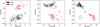 |
Fig. 8. Distributions of the VOD, HAC and EriPhe in the (X, Y), (X, Z), and (Y, Z). Arrows indicate the velocity direction and the length of arrows show the size of velocity of the members. Black color presents VOD, red color presents HAC, and the blue circle indicates EriPhe. The big black dot represents Galactic centre. |
Boubert et al. (2019) suggested that a part of the VOD region may be Small Magellanic Cloud (SMC) debris from a tidal interaction of the SMC and Large Magellanic Cloud (LMC) 3 Gyr ago. These authors also gave ten random orbital tracks for the LMC and SMC from present day to 1 Gyr in the future, which were found to pass through the region of VOD. We selected the member stars of SMC and LMC from APOGEE DR17 using Teff, log g, radial velocity, and proper motions according to the selection criteria provided by Nidever et al. (2020). We compared the distribution of [α/Fe] and [Fe/H] of VOD and SMC, LMC in Fig. 9. In the lower panels, we found that the distribution of [Fe/H] and α elements of VOD is closer to that of LMC and SMC. In the upper panels, we can see the overlap between SMC and VOD is more than that of LMC and VOD. We thus support the conclusion of Boubert et al. (2019) that VOD may be the debris of SMC 3 Gyr ago.
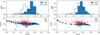 |
Fig. 9. Comparison of elements abundance between VOD and LMC, SMC. Top: histogram distribution of elements abundance in VOD, SMC and LMC regions. The solid black line indicates VOD, the blue indicates SMC and LMC. Bottom: distribution of α elements with [Fe/H]. The red dots indicate VOD members and the blue dots indicate the stars in LMC and SMC regions. The big black dotted line represents the trend line of abundance of LMC and SMC from Nidever et al. (2020). |
5. Conclusions
We selected member stars of VOD and HAC from the K giant sample in Yang et al. (2019) and cross-match these member stars with Xiang et al. (2019) to obtain the elemental abundances. We investigated the relationship between VOD and HAC from both the kinematic and chemical point of view, with the following conclusions:
1. Although the VOD and HAC regions are distributed diagonally relative to each other in terms of spatial position distribution, they mix with each other in velocity space and their average velocities and dispersions are similar.
2. The distributions of orbital eccentricity between VOD and HAC are very consistent, and their member stars are basically at e > 0.7. Meanwhile, other orbital parameters are also similar, indicating that they may have the same nature in the orbits, which is consistent with the conclusions of Simion et al. (2019).
3. In terms of energy and angular momentum, both the VOD and HAC are in low-angular-momentum and high-energy orbits, and their motions show the same trend. We calculated the density distribution of the spatial positions of these two structures for the past 8 Gyr, finding very similar distributions.
4. We find that it is impossible to distinguish the two structures from the distributions of many elemental abundances, suggesting that they may have the same chemical evolution. The conclusion that they share a common origin is thereby strengthened.
5. Based on kinematics and abundances, the VOD and HAC may come from a large dwarf galaxy merger, possibly that of GSE (Zhao & Chen 2021) or a splash event (Belokurov et al. 2020). From the elemental abundances, parts of the VOD may be closely related to SMC debris that was stripped away 3 Gyr ago.
Acknowledgments
This work was supported by the National Natural Science Foundation of China under grant Nos. 11988101, 11890694, 12273055, 11973048, 11927804 and National Key R&D Program of China No. 2019YFA0405502. We acknowledge the science research grants from the China Manned Space Project CSST. We thank Ji Li and Guang Mei Wang for their meaningful discussion. Guoshoujing Telescope (the Large Sky Area Multi-Object Fiber Spectroscopic Telescope LAMOST) is a National Major Scientific Project built by the Chinese Academy of Sciences. Funding for the project has been provided by the National Development and Reform Commission. LAMOST is operated and managed by the National Astronomical Observatories, Chinese Academy of Sciences. We thank the galpy (http://github.com/jobovy/galpy) python package for providing us with the tools to compute kinematic information on the member stars.
References
- Astropy Collaboration (Price-Whelan, A. M., et al.) 2018, AJ, 156, 123 [Google Scholar]
- Belokurov, V., Zucker, D. B., Evans, N. W., et al. 2006, ApJ, 642, L137 [Google Scholar]
- Belokurov, V., Zucker, D. B., Evans, N. W., et al. 2007, ApJ, 654, 897 [Google Scholar]
- Belokurov, V., Sanders, J. L., Fattahi, A., et al. 2020, MNRAS, 494, 3880 [Google Scholar]
- Boubert, D., Belokurov, V., Erkal, D., & Iorio, G. 2019, MNRAS, 482, 4562 [NASA ADS] [CrossRef] [Google Scholar]
- Bovy, J. 2015, ApJS, 216, 29 [NASA ADS] [CrossRef] [Google Scholar]
- Bullock, J. S., & Johnston, K. V. 2005, ApJ, 635, 931 [Google Scholar]
- Carlin, J. L., Yam, W., Casetti-Dinescu, D. I., et al. 2012, ApJ, 753, 145 [NASA ADS] [CrossRef] [Google Scholar]
- Cui, X.-Q., Zhao, Y.-H., Chu, Y.-Q., et al. 2012, Res. Astron. Astrophys., 12, 1197 [Google Scholar]
- Donlon, T., Newberg, H. J., Weiss, J., Amy, P., & Thompson, J. 2019, ApJ, 886, 76 [NASA ADS] [CrossRef] [Google Scholar]
- Duffau, S., Vivas, A. K., Zinn, R., Méndez, R. A., & Ruiz, M. T. 2014, A&A, 566, A118 [NASA ADS] [CrossRef] [EDP Sciences] [Google Scholar]
- Han, J. J., Naidu, R. P., Conroy, C., et al. 2022, ApJ, 934, 14 [CrossRef] [Google Scholar]
- Iorio, G., & Belokurov, V. 2019, MNRAS, 482, 3868 [NASA ADS] [CrossRef] [Google Scholar]
- Ivezić, Ž., Goldston, J., Finlator, K., et al. 2000, AJ, 120, 963 [CrossRef] [Google Scholar]
- Jurić, M., Ivezić, Ž., Brooks, A., et al. 2008, ApJ, 673, 864 [Google Scholar]
- Li, T. S., Balbinot, E., Mondrik, N., et al. 2016, ApJ, 817, 135 [NASA ADS] [CrossRef] [Google Scholar]
- Majewski, S. R., Skrutskie, M. F., Weinberg, M. D., & Ostheimer, J. C. 2003, ApJ, 599, 1082 [NASA ADS] [CrossRef] [Google Scholar]
- Newberg, H. J., Yanny, B., Rockosi, C., et al. 2002, ApJ, 569, 245 [Google Scholar]
- Nidever, D. L., Hasselquist, S., Hayes, C. R., et al. 2020, ApJ, 895, 88 [Google Scholar]
- Perottoni, H. D., Limberg, G., Amarante, J. A. S., et al. 2022, ApJ, 936, L2 [NASA ADS] [CrossRef] [Google Scholar]
- Rocha-Pinto, H. J., Majewski, S. R., Skrutskie, M. F., & Crane, J. D. 2003, ApJ, 594, L115 [NASA ADS] [CrossRef] [Google Scholar]
- Schönrich, R., Binney, J., & Dehnen, W. 2010, MNRAS, 403, 1829 [NASA ADS] [CrossRef] [Google Scholar]
- Searle, L., & Zinn, R. 1978, ApJ, 225, 357 [Google Scholar]
- Shi, W. B., Chen, Y. Q., Carrell, K., & Zhao, G. 2012, ApJ, 751, 130 [NASA ADS] [CrossRef] [Google Scholar]
- Simion, I. T., Belokurov, V., Irwin, M., & Koposov, S. E. 2014, MNRAS, 440, 161 [NASA ADS] [CrossRef] [Google Scholar]
- Simion, I. T., Belokurov, V., Koposov, S. E., Sheffield, A., & Johnston, K. V. 2018, MNRAS, 476, 3913 [NASA ADS] [CrossRef] [Google Scholar]
- Simion, I. T., Belokurov, V., & Koposov, S. E. 2019, MNRAS, 482, 921 [NASA ADS] [CrossRef] [Google Scholar]
- Skrutskie, M. F., Cutri, R. M., Stiening, R., et al. 2006, AJ, 131, 1163 [NASA ADS] [CrossRef] [Google Scholar]
- Spergel, D. N., Verde, L., Peiris, H. V., et al. 2003, ApJS, 148, 175 [Google Scholar]
- Vivas, A. K., Zinn, R., Andrews, P., et al. 2001, ApJ, 554, L33 [NASA ADS] [CrossRef] [Google Scholar]
- Vivas, A. K., Zinn, R., Farmer, J., Duffau, S., & Ping, Y. 2016, ApJ, 831, 165 [NASA ADS] [CrossRef] [Google Scholar]
- Xiang, M., Ting, Y.-S., Rix, H.-W., et al. 2019, ApJS, 245, 34 [Google Scholar]
- Yang, C., Xue, X.-X., Li, J., et al. 2019, ApJ, 880, 65 [NASA ADS] [CrossRef] [Google Scholar]
- Yanny, B., Newberg, H. J., Kent, S., et al. 2000, ApJ, 540, 825 [NASA ADS] [CrossRef] [Google Scholar]
- York, D. G., Adelman, J., Anderson, J. E. Jr., et al. 2000, AJ, 120, 1579 [Google Scholar]
- Zhang, X., Shi, W. B., Chen, Y. Q., et al. 2017, A&A, 597, A54 [NASA ADS] [CrossRef] [EDP Sciences] [Google Scholar]
- Zhao, G., & Chen, Y. 2021, Sci. China Phys. Mech. Astron., 64, 239562 [NASA ADS] [CrossRef] [Google Scholar]
- Zhao, G., Chen, Y.-Q., Shi, J.-R., et al. 2006, Chin. J. Astron. Astrophys., 6, 265 [NASA ADS] [CrossRef] [Google Scholar]
- Zhao, G., Zhao, Y.-H., Chu, Y.-Q., et al. 2012, Res. Astron. Astrophys., 12, 723 [CrossRef] [Google Scholar]
- Zinn, R., Horowitz, B., Vivas, A. K., et al. 2014, ApJ, 781, 22 [NASA ADS] [CrossRef] [Google Scholar]
All Tables
All Figures
|
Fig. 1. Distributions of the two fields (VOD and HAC) in the (l, b), (X–Y), (X–Z) space. Black dots: member stars of VOD. Red dots: member stars of HAC. |
| In the text | |
|
Fig. 2. Velocity distribution in spherical polar coordinates (Vr, Vϕ, and Vθ are the radial, azimuthal, and polar components, in km s−1) of the VOD and HAC. Upper panels: scatter diagrams of the velocity distributions of the VOD (black) and HAC (red). Lower panels: histograms displaying the velocity distributions of VOD (black) and HAC (red) members. |
| In the text | |
|
Fig. 3. Properties of the stellar orbits in the VOD and HAC fields. Upper panels: maximal height above the galactic plane, apocentre, and Galactocentric radius as a function of eccentricity, for the VOD (black) and HAC (red) stars. Lower panels: histogram distribution of eccentricity, apocentre, and Galactocentric distance. |
| In the text | |
|
Fig. 4. Distribution of the angular momentum and the energy in the VOD (black dots) and HAC (red dots) regions. |
| In the text | |
|
Fig. 5. Density maps of the member stars along their individual orbits over the past 8 Gyr, in Galactic coordinates (left panels) and in the X–Y (middle) and Y–Z (right). |
| In the text | |
|
Fig. 6. Histogram distribution of elements abundance. Solid black line indicates VOD members and the red dashed line indicates HAC members. |
| In the text | |
|
Fig. 7. Distribution of element abundances with [Fe/H] and the distribution of the radial velocity with [Fe/H]. |
| In the text | |
|
Fig. 8. Distributions of the VOD, HAC and EriPhe in the (X, Y), (X, Z), and (Y, Z). Arrows indicate the velocity direction and the length of arrows show the size of velocity of the members. Black color presents VOD, red color presents HAC, and the blue circle indicates EriPhe. The big black dot represents Galactic centre. |
| In the text | |
|
Fig. 9. Comparison of elements abundance between VOD and LMC, SMC. Top: histogram distribution of elements abundance in VOD, SMC and LMC regions. The solid black line indicates VOD, the blue indicates SMC and LMC. Bottom: distribution of α elements with [Fe/H]. The red dots indicate VOD members and the blue dots indicate the stars in LMC and SMC regions. The big black dotted line represents the trend line of abundance of LMC and SMC from Nidever et al. (2020). |
| In the text | |
Current usage metrics show cumulative count of Article Views (full-text article views including HTML views, PDF and ePub downloads, according to the available data) and Abstracts Views on Vision4Press platform.
Data correspond to usage on the plateform after 2015. The current usage metrics is available 48-96 hours after online publication and is updated daily on week days.
Initial download of the metrics may take a while.