| Issue |
A&A
Volume 673, May 2023
|
|
|---|---|---|
| Article Number | A27 | |
| Number of page(s) | 12 | |
| Section | Stellar structure and evolution | |
| DOI | https://doi.org/10.1051/0004-6361/202346084 | |
| Published online | 27 April 2023 | |
Photometry and spectroscopy of the Type Icn supernova 2021ckj
The diverse properties of the ejecta and circumstellar matter of Type Icn supernovae⋆
1
Department of Physics and Astronomy, University of Turku, 20014 Turku, Finland
e-mail: This email address is being protected from spambots. You need JavaScript enabled to view it.
2
Aalto University Metsähovi Radio Observatory, Metsähovintie 114, 02540 Kylmälä, Finland
3
Aalto University Department of Electronics and Nanoengineering, PO Box 15500 00076 Aalto, Finland
4
Finnish Centre for Astronomy with ESO (FINCA), University of Turku, 20014 Turku, Finland
5
Department of Astronomy, Kyoto University, Kitashirakawa-Oiwake-cho, Sakyo-ku, Kyoto 606-8502, Japan
6
Astrophysics Research Centre, School of Mathematics and Physics, Queens University Belfast, Belfast BT7 1NN, UK
7
INAF – Osservatorio Astronomico di Padova, Vicolo dell’Osservatorio 5, 35122 Padova, Italy
8
School of Sciences, European University Cyprus, Diogenes street, Engomi, 1516 Nicosia, Cyprus
9
Facultad de Ciencias Astronómicas y Geofísicas, Universidad Nacional de La Plata, Paseo del Bosque s/n, B1900FWA La Plata, Argentina
10
Instituto de Astrofísica de La Plata (IALP), CONICET, Argentina
11
European Southern Observatory, Alonso de Córdova 3107, Casilla 19, Santiago, Chile
12
Millennium Institute of Astrophysics MAS, Nuncio Monsenor Sotero Sanz 100, Off. 104, Providencia, Santiago, Chile
13
Technische Universität München, TUM School of Natural Sciences, Physik-Department, James-Franck-Straße 1, 85748 Garching, Germany
14
Max-Planck-Institut für Astrophysik, Karl-Schwarzschild Straße 1, 85748 Garching, Germany
15
Institute of Space Sciences (ICE, CSIC), Campus UAB, Carrer de Can Magrans, s/n, 08193 Barcelona, Spain
16
Institut d’Estudis Espacials de Catalunya (IEEC), 08034 Barcelona, Spain
17
Institute for Astronomy, University of Hawaii, 2680 Woodlawn Drive, Honolulu, HI 96822, USA
18
Astronomical Observatory, University of Warsaw, Al. Ujazdowskie 4, 00-478 Warszawa, Poland
19
Cardiff Hub for Astrophysics Research and Technology, School of Physics & Astronomy, Cardiff University, Queens Buildings, The Parade, Cardiff CF24 3AA, UK
20
Turku Collegium for Science, Medicine and Technology, University of Turku, 20014 Turku, Finland
21
Institute of Astronomy, University of Hawaii, 2680 Woodlawn Drive, Honolulu, HI 96822, USA
22
Instituto de Astrofísica, Departamento de Física – Universidad Andres Bello, Avda. República 252, 8320000 Santiago, Chile
Received:
6
February
2023
Accepted:
13
March
2023
Abstract
We present photometric and spectroscopic observations of the Type Icn supernova (SN) 2021ckj. This rare type of SNe is characterized by a rapid evolution and high peak luminosity as well as narrow lines of highly ionized carbon at early phases, implying an interaction with hydrogen- and helium-poor circumstellar matter (CSM). SN 2021ckj reached a peak brightness of ∼ − 20 mag in the optical bands, with a rise time and a time above half maximum of ∼4 and ∼10 days, respectively, in the g and cyan bands. These features are reminiscent of those of other Type Icn SNe (SNe 2019hgp, 2021csp, and 2019jc), with the photometric properties of SN 2021ckj being almost identical to those of SN 2021csp. Spectral modeling of SN 2021ckj reveals that its composition is dominated by oxygen, carbon, and iron group elements, and the photospheric velocity at peak is ∼10 000 km s−1. Modeling the spectral time series of SN 2021ckj suggests aspherical SN ejecta. From the light curve (LC) modeling applied to SNe 2021ckj, 2019hgp, and 2021csp, we find that the ejecta and CSM properties of Type Icn SNe are diverse. SNe 2021ckj and 2021csp likely have two ejecta components (an aspherical high-energy component and a spherical standard-energy component) with a roughly spherical CSM, while SN 2019hgp can be explained by a spherical ejecta-CSM interaction alone. The ejecta of SNe 2021ckj and 2021csp have larger energy per ejecta mass than the ejecta of SN 2019hgp. The density distribution of the CSM is similar in these three SNe, and is comparable to those of Type Ibn SNe. This may imply that the mass-loss mechanism is common between Type Icn (and also Type Ibn) SNe. The CSM masses of SN 2021ckj and SN 2021csp are higher than that of SN 2019hgp, although all these values are within those seen in Type Ibn SNe. The early spectrum of SN 2021ckj shows narrow emission lines from C II and C III, without a clear absorption component, in contrast with that observed in SN 2021csp. The similarity of the emission components of these lines implies that the emitting regions of SNe 2021ckj and 2021csp have similar ionization states, and thus suggests that they have similar properties as the ejecta and CSM, which is also inferred from the LC modeling. Taking the difference in the strength of the absorption features into account, this heterogeneity may be attributed to viewing angle effects in otherwise common aspherical ejecta. In particular, in this scenario SN 2021ckj is observed from the polar direction, while SN 2021csp is seen from an off-axis direction. This is also supported by the fact that the late-time spectra of SNe 2021ckj and 2021csp show similar features but with different line velocities.
Key words: supernovae: general / supernovae: individual: SN 2021ckj / circumstellar matter
All the spectroscopic data presented in this paper are available at the Weizmann Interactive Supernova Data Repository (WISeREP; https://www.wiserep.org/object/17712; Yaron & Gal-Yam 2012). The photometric data are presented in Table 2.
© The Authors 2023
 Open Access article, published by EDP Sciences, under the terms of the Creative Commons Attribution License (https://creativecommons.org/licenses/by/4.0), which permits unrestricted use, distribution, and reproduction in any medium, provided the original work is properly cited.
This article is published in open access under the Subscribe to Open model. This email address is being protected from spambots. You need JavaScript enabled to view it. to support open access publication.
1. Introduction
A new class of supernovae (SNe) has been recently proposed based on the observations of SN 2019hgp (Type Icn SNe; Gal-Yam et al. 2022). These SNe are characterized by a rapid photometric evolution (trise ≲ 10 days) with a high peak brightness (r ∼ −18.5 mag) as well as narrow P-Cygni lines of highly ionized carbon, oxygen, and neon in its early spectra (Gal-Yam et al. 2022). Recently, several more examples, which show similar observational properties, have been reported (SNe 2019jc, 2021csp, 2021ckj, and 2022ann; Fraser et al. 2021; Perley et al. 2022; Pellegrino et al. 2022; Davis et al. 2022). The narrow lines of such highly ionized elements suggest an interaction of the SN ejecta with dense hydrogen- and helium-poor circumstellar matter (CSM).
Fraser et al. (2021) estimate that the bolometric light curve (LC) of SN 2021csp can be reproduced by a 4 × 1051 erg explosion with 2 M⊙ of ejecta and 0.4 M⊙ of 56Ni, plus a contribution from shock cooling emission of ∼1 M⊙ of CSM extending out to 400 R⊙. However, from their LC analysis of SN 2021csp, Perley et al. (2022) and Pellegrino et al. (2022) favor a CSM interaction as the main energy source of this SN. Gal-Yam et al. (2022) also demonstrate that the bolometric LC of SN 2019hgp is well fit by a CSM interaction model (a progenitor radius of 4.1 × 1011 cm, an ejecta mass of 1.2 M⊙, an opacity of 0.04 cm2 g−1, a CSM mass of 0.2 M⊙, a mass-loss rate of 0.004 M⊙ yr−1, and an expansion speed of 1900 km s−1) rather than models with an energy input from the radioactive decay of 56Ni/56Co.
Since Type Icn SNe do not show hydrogen or helium features in their spectra, their progenitors are believed to be stars whose hydrogen and helium envelopes were stripped, as inferred for the progenitors of classical Type Ic SNe. Therefore, a straightforward scenario for the origin of Type Icn SNe would be a similar progenitor star as those of classical Type Ic SNe, exploding just after an extensive mass ejection, even though the progenitors of classical Type Ic SNe are also under debate (see, e.g., Yoon 2015, and references therein). However, Perley et al. (2022) estimate a minimal 56Ni mass and/or a low ejecta mass from their late-time deep photometry for SN 2021csp, and they conclude that its progenitor is intrinsically different from those of classical Type Ic SNe. This conclusion is also supported by Pellegrino et al. (2022), who infer low ejecta masses (≲2 M⊙) and low 56Ni masses (≲0.04 M⊙) from the LCs of four Type Icn SNe. These values are lower than typical 56Ni masses (∼0.2 M⊙) and ejecta masses (∼2 M⊙) estimated for Type Ic SNe (e.g., Drout et al. 2011).
There are several proposed scenarios for the origin of Type Icn SNe (e.g., Fraser et al. 2021; Perley et al. 2022). These include, for example: (1) an SN from a highly stripped star in a binary system (e.g., De et al. 2018; Sawada et al. 2022); (2) a pulsational pair-instability SN (PPISN; e.g., Woosley 2017); (3) a merger of a Wolf-Rayet (WR) star and a compact object (e.g., Metzger 2022); and (4) a failed or partial explosion of a WR star, in which a direct collapse of a WR star to a black hole launches a subrelativistic jet, and the jet interacts with a dense CSM releasing the radiated energy (e.g., Perley et al. 2022). Gal-Yam et al. (2022) propose a WR star to be the progenitor of SN 2019hgp based on its observational properties, and suggest a possibility that the differences between Type Ibn and Icn SNe arise from their different types of WR star progenitors: helium- and nitrogen-rich WN stars for Type Ibn SNe and C-rich WC stars for Type Icn SNe. Pellegrino et al. (2022) propose that multiple progenitor channels could explain different Type Icn SNe, based on the properties of the SNe and their explosion sites. They suggest that the progenitor of SN 2019jc was a low-mass, ultra-stripped star, whereas those of SNe 2019hgp, 2021csp, and 2021ckj were WR stars. Furthermore, Davis et al. (2022) suggest a binary-stripped progenitor for SN 2022ann, rather than a single massive WR progenitor.
In this paper, we report photometric and spectroscopic observations of the Type Icn SN 2021ckj and discuss its observational properties as compared to those of SNe 2019hgp and 2021csp, the two most well-observed members of this class. SN 2021ckj was discovered as ZTF21aajbgol by the Zwicky Transient Facility (ZTF; Bellm et al. 2019) on 9.29 February 2021 UT (59254.29 MJD), which was reported by the Automatic Learning for the Rapid Classification of Events (ALeRCE; Förster et al. 2021). The object was not detected down to a limiting magnitude of 20.7 mag on 7.36 February 2021 UT (59252.36 MJD), as constrained by the Asteroid Terrestrial impact Last Alert System (ATLAS; Tonry et al. 2018; Smith et al. 2020). We adopt the middle point between the discovery and the last nondetection, 59253.38 MJD, as the explosion date. The phases in this paper are shown in rest-frame days with respect to this explosion date. The spectroscopic classification of SN 2021ckj as a Type Icn SN was conducted on 16 February 2021 by Pastorello et al. (2021), based on a spectrum taken with the ESO Very Large Telescope (VLT) and the FORS2 spectrograph.
Throughout this paper, we adopt a redshift z = 0.141 (measured from the narrow host-galaxy emission lines), and a distance modulus μ = 39.04 mag (assuming H0 = 73 km s−1 Mpc−1, Ωm = 0.27, and ΩΛ = 0.73). Since the spectra of SN 2021ckj show no signs of narrow Na I D interstellar absorption, we assume that it has a minimal host-galaxy extinction (see Sect. 2.2). Only the Galactic extinction correction has been performed to the photometric and spectroscopic data, assuming E(B − V) = 0.049 (Schlafly & Finkbeiner 2011), RV = 3.1, and the extinction curve by Cardelli et al. (1989) using IRAF (Tody 1986, 1993).
2. Observations
2.1. Photometry
SN 2021ckj was observed by several wide-field transient surveys, such as ZTF, ATLAS, and the Panoramic Survey Telescope and Rapid Response System (Pan-STARRS; Chambers et al. 2016). We obtained g-, r-, and i-band images taken by ZTF through the NASA/IPAC Infrared Science Archive1. We also used the “cyan”-band photometry reported by ATLAS, and “white”-band photometry by Pan-STARRS. We conducted multiband (uBVgRriz) photometry of SN 2021ckj with the EFOSC2 instrument mounted on the New Technology Telescope (NTT) at La Silla Observatory in Chile as a part of the extended Public ESO Survey for Transient Objects (ePESSTO+; Smartt et al. 2015), as well as the AFOSC instrument mounted on the Copernico Telescope. The observation log is shown in Table 1.
Log of the photometry of SN 2021ckj.
We reduced the data using the PESSTO pipeline (Smartt et al. 2015) and IRAF, performing standard tasks such as bias subtraction and flat-fielding. For the EFOSC2 data, we performed point-spread function (PSF) photometry after host galaxy subtraction with reference images taken on 3 February 2022; whereas, for the other data, we conducted PSF photometry with the stacked Pan-STARRS g-, r-, and i-band images as reference images. A correction for the Galactic extinction was applied. The resulting photometry is provided in Table 2.
Photometry of SN 2021ckj.
2.2. Spectroscopy
The first spectrum of SN 2021ckj was obtained by Pastorello et al. (2021) at Phase +7.7 days with the FORS2 instrument (Appenzeller et al. 1998) at the ESO VLT with the 300V grism and a 1 arcsec slit width. We took another spectrum at Phase +12.1 days with EFOSC2/NTT using the Gr#13 grism and a 1 arcsecond slit width as a part of the ePESSTO+ collaboration (Smartt et al. 2015). In addition, we obtained one more spectrum at Phase +21.2 d using FORS2/VLT with grism 300V.
The EFOSC2 and FORS2 data were reduced using the PESSTO2 and ESOReflex (Freudling et al. 2013) pipelines, respectively, which include standard tasks such as bias subtraction, flat-fielding, and a wavelength calibration based on arc frames. The flux calibration was performed using observations of a spectrophotometric standard star.
3. Results
3.1. Photometric properties
Figure 1 shows multiband LCs of SN 2021ckj. They show bright peak brightness and rapid rises and declines. The absolute peak magnitudes are ∼ − 20 mag in the optical bands (e.g., g, cyan, and r bands). The rise time and the time above half maximum (t1/2) are ∼4 and ∼10 days, respectively, in the g and cyan bands. These features are similar to other Type Icn SNe (SNe 2019hgp, 2021csp, and 2019jc; Fraser et al. 2021; Gal-Yam et al. 2022; Perley et al. 2022; Pellegrino et al. 2022). Especially, the LCs of SN 2021ckj are almost replicas of SN 2021csp around the peaks (see their r-band LCs in Fig. 1), although they deviate from each other at later phases.
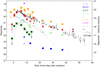 |
Fig. 1. Optical LCs of SN 2021ckj. The data were taken with the 1.82 m Copernico Telescope (triangles), NTT (circles), ZTF (filled squares), ATLAS (inverted triangles), and Pan-STARRS (diamonds). The R-band magnitudes in the NTT data have been converted into r-band magnitudes using the relation in Chonis & Gaskell (2008). The gray and black points show the r-band LCs of SNe 2019hgp (Gal-Yam et al. 2022) and 2021csp (Fraser et al. 2021), respectively, which have been plotted using their absolute magnitudes. Limiting magnitudes are indicated with arrows. All the magnitudes have been corrected with the Galactic extinction (E(B − V) = 0.027 and 0.019 mag for SNe 2021csp and 2019hgp, respectively; Schlafly & Finkbeiner 2011). The error bars for all data points have also been plotted, even though they are smaller than the sizes of the symbols in most cases. |
First, we calculated the blackbody (BB) radius and temperature for the SN radiation at Phase +8.38 through χ2 fits of the uBVgriz-band photometry with the Planck function. Since the photometric data in the other phases are limited, the wavelength ranges of the observations do not cover the peaks of BB curves with anticipated temperatures (∼10 000 K). In fact, similar χ2 fittings for the other phases produce poor constraints on their BB radii and temperatures. Therefore, we performed the χ2 fittings with the fixed temperature estimated from Phase +8.38 for the other phases. Here, we did not use the data at Phase 12.07, which has only one band of photometry. From the derived BB parameters, we calculated the bolometric luminosity by integrating the BB function across wavelengths. The estimated values are shown in Fig. 2. The derived luminosities, radii, and temperatures for SN 2021ckj are very similar to those for SN 2021csp, while they have a different evolution from those of SN 2019hgp.
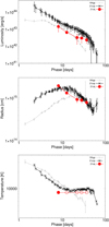 |
Fig. 2. Evolution of the photospheric parameters estimated from blackbody fitting to the photometry of SN 2021ckj (red points connected with a line). Open red circles are the assumed values. Comparison objects, SNe 2019hgp and 2021csp, are shown with the gray and black points connected with lines, respectively. The values for the comparison objects have been taken from Gal-Yam et al. (2022) and Fraser et al. (2021). |
3.2. Spectroscopic properties
In the early spectrum of SN 2021ckj (Phase +7.7 days), there are highly ionized narrow lines of C II/C III, which are also seen in the spectra of SNe 2019hgp and 2021csp at similar epochs (Phases +10.8 and +7.9 days, respectively; see Fig. 3). This indicates that the CSM has a similar ionization state at similar epochs for these SNe. SN 2021ckj shows minimal absorption for strong C II lines (e.g., C II λ5890 and 6578), while SNe 2019hgp and 2021csp show an evident blueshifted absorption component for the C II lines. The second spectrum of SN 2021ckj (Phase +12.1 days) is smooth and featureless, similar to other Type Icn SNe around this phase; although, the signal-to-noise ratio of the spectrum is not high (see Fig. 3).
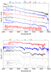 |
Fig. 3. Spectral evolution of SN 2021ckj. Top panel: early spectra of SN 2021ckj (red), compared with the other Type Icn SNe 2019hgp (gray) and 2021csp (black). Bottom panel: same as the top panel, but for the late-time spectra. For comparison, the spectra of SNe 2020bqj (Ibn; Kool et al. 2021), 2020uem (IIn/Ia-CSM; Uno et al. 2023), and 2021foa (IIn; Reguitti et al. 2022) are plotted. These data were obtained through WISeREP (https://www.wiserep.org/object/17712). |
The late-time spectrum of SN 2021ckj (Phase +21.2 days) shows a blue pseudo-continuum due to Fe lines with some undulations at λ ≲ 5500 Å (so-called Fe bump), while no evident lines are visible in the red part, except for the Ca II NIR triplet (see Fig. 3). This Fe bump is also seen in other interacting SNe, for example Type Ibn (e.g., Pastorello et al. 2016), Type Ia-CSM (e.g., Fox et al. 2015), some Type IIn SNe (e.g., Turatto et al. 1993), and interacting Type-Ic SNe (Kuncarayakti et al. 2018, 2022). On the other hand, SNe 2019hgp and 2021csp show more line features while showing a similar “Fe bump”. The narrow line seen near the Hα wavelength in the late-time spectrum of SN 2021ckj could be identified with C II λ6578.
It is intriguing that the overall spectra are similar among these Type Icn SNe, while the difference is seen in the line profiles and velocities, both in the early and late phases. This is one of the topics that we address in the present work; we suggest that the difference seen in the line features might be due to different ejecta velocities and/or viewing angle effects due to an aspherical explosion.
4. LC modeling
In this section, we model the bolometric LCs of SNe 2021ckj, 2021csp, and 2019hgp using the CSM interaction model of Maeda & Moriya (2022), in order to estimate their ejecta and CSM properties. In the calculations, we adopt the following broken power law for the density structure of the SN ejecta as a function of velocity (v); ρSN ∝ v−n and n = 7 is used for the outer part, and a constant density is used for the inner part. The normalization in the density is set by specifying the ejecta mass (Mej) and the explosion energy (EK). For the CSM, a single power-law function of the distance (r) is assumed using constant values, D, D′, and s; ρCSM = Dr−s = 10−14D′(r/5 × 1014 cm)−s g cm−3. For Type Ibn SNe, Maeda & Moriya (2022) derived s ∼ 2.5 − 3.0 and D′∼0.5 − 5. The mass-loss rate responsible for the CSM at the reference radius, 5 × 1014 cm (which corresponds to the position of the shock wave on day 2 for the shock velocity of 30 000 km s−1), is Ṁ ∼ 0.05D′(vw/1000 km s−1) M⊙ yr−1, where vw is the mass-loss wind velocity. We assume a C+O-rich composition, but the optical LC models explored here are not sensitive to the choice of the composition as the main power in the model is provided by the free–free emission at the high-temperature forward shock. Also, we note that our models are not aimed to provide a unique solution for the model parameters.
The model LCs and characteristic-radius evolution are shown in Fig. 4. The radius shown here is the position of the contact discontinuity, that is the representative scale of the interacting region, which provides the maximum radius expected in the interaction model. The photosphere radius is expected to be either close to this radius (if the shocked region is optically thick to the optical photons) or smaller (if the shocked region is optically thin). The model assumes spherical symmetry both in the ejecta and the CSM. Possible effects of asymmetry in the ejecta, as indicated by the spectral features in these objects, are discussed in Sect. 6.
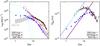 |
Fig. 4. LC models (left panel) and evolution of the radius at the contact discontinuity, as compared to the photospheric radius (right panel). The model parameters are as follows: Mej = 3M⊙, EK = 2.5 × 1051 ergs, s = 2.9, and D′ = 2.3 for SN 2019hgp (blue lines), and Mej = 4 M⊙, EK = 4 × 1051 ergs, s = 2.9, and D′ = 5.1 for SNe 2021ckj and 2021csp (red lines). Additionally, two scenarios for the initial decay seen in SN 2021csp are shown: (1) the SN-CSM interaction driven by a highly energetic component (magenta lines) and (2) the shock-cooling of an energetic component (solid cyan lines). As a comparison, the same is also shown, but for a canonical explosion energy (dashed-cyan line). The gray hatching shows the template of the LCs of Type Ibn SNe (Hosseinzadeh et al. 2017; Maeda & Moriya 2022). |
4.1. SN 2019hgp
Our first attempt is made for SN 2019hgp. Given the close similarity of its LC to the Type Ibn SN template (see Fig. 4), a good match to its LC is obtained with the ejecta and CSM properties similar to those applied for Type Ibn SNe by Maeda & Moriya (2022, Mej ∼ 2 − 6 M⊙, EK ∼ 1 × 1051 ergs, s ∼ 2.5 − 3.0, and D′∼0.5 − 5.0); Mej = 3 M⊙, EK = 2.5 × 1051 ergs, s = 2.9, and D′ = 2.3 for SN 2019hgp (blue line). The evolution of the radius of the shocked region roughly follows the BB radius up to ∼10 − 20 days (it is important to note that we do not model the first 4 or 5 days in detail, as this would require a more detailed treatment of radiation transfer effects). Interestingly, the photosphere starts receding at ∼10 − 20 days, which coincides with the kink seen in the LC evolution. This transition in the LC from a flat to steep evolution is interpreted as being caused by the change in the forward-shock property from the optically thick cooling phase to the optically thin adiabatic phase (see Maeda & Moriya 2022). According to this interpretation, we expect that the photosphere is formed in the shocked region in the earlier phases, but it later recedes into the ejecta once the shock becomes optically thin. This interpretation is consistent with the spectral evolution from the CSM interaction-dominated phase (characterized by a featureless blue continuum with narrow lines) into the SN ejecta-dominated one (with a broad-line spectrum; see Fig. 3). The simultaneous occurrence of the accelerated LC decay and the spectral evolution due to the receding photosphere is predicted by the model of Maeda & Moriya (2022), strengthening the case that SN 2019hgp is mainly powered by the SN-CSM interaction.
4.2. SNe 2021csp and 2021ckj
The LC of SN 2021csp shows an initial rapid-decay phase, followed by a flattening (> 10 days) and then again by a steep decay (> 40 days). SN 2021ckj might show similar evolution to SN 2021csp, even though the data have not been sampled enough in the earliest and latest phases. Since the photometric and spectroscopic properties of SNe 2021csp and 2021ckj are very similar (see Sect. 3), we assume that they are “twins” and model the LC of SN 2021csp to understand both SNe. The initial decay is not predicted directly in the SN-CSM interaction model that assumes a single power-law CSM distribution. Thus, we discuss this part separately in Sect. 4.3. The LC evolution, except for this initial decay (≳10 days), is similar to the evolution seen in the Type Ibn SN template, but it is somewhat brighter and has a slower transition. The model shown in Fig. 4 (red line) has the following parameters: Mej = 4 M⊙, EK = 4 × 1051 ergs, s = 2.9, and D′ = 5.1. As compared to the models for Type Ibn SNe and SN 2019hgp, the ejecta and CSM properties of these SNe are slightly different: the energy per ejecta mass is larger and the CSM density is on a higher side, although the total ejecta mass and the CSM density distribution are similar.
4.3. The initial rapid-declining phase of SN 2021csp
As mentioned above, in the early phase, the LC of SN 2021csp shows different properties from those of SN 2019hgp and Type Ibn SNe. It exhibits a rapidly declining LC after maximum as well as a very high photospheric velocity of ∼30 000 km s−1, estimated from the time evolution of the BB radius (cyan line in the right-hand side panel of Fig. 4). In addition, the photosphere already starts to recede at ∼5 days, which is earlier than seen for SN 2019hgp (∼20 days; see Fig. 4). These properties are difficult to reconcile with those at later phases in the present CSM-interaction model. In particular, the initial very high photospheric velocity contradicts the bright and slow LC evolution at later phases. Although the latter requires a large amount of CSM, this should substantially decelerate the shock wave, causing a challenge in reproducing the early high velocity. This may indicate that the initial phase is powered by a different mechanism. We consider two scenarios: (1) a CSM interaction by a highly energetic ejecta component in addition to the interaction by slower ejecta at later phases; and (2) the initial phase not being powered by an instantaneous interaction, but by a mechanism similar to the shock-cooling emission. In the former scenario, it is assumed that the SN-CSM interaction is ongoing in an optically thin environment, and the kinetic energy dissipated at the shock front is immediately converted to optical radiation as it is observed. In the latter scenario, most of the kinetic energy is dissipated early on before the observation, either within the progenitor’s envelope or optically thick CSM, after that the dissipated energy is converted to thermal energy and forms an expanding fireball; the subsequent radiation loss in the cooling fireball ultimately produces the characteristic “shock-cooling” emission.
4.3.1. CSM interaction scenario
To support scenario (1), we show an additional model (magenta line) in which only EK is changed from the reference model for the later phase of SNe 2021csp and 2021ckj, while the other parameters are unchanged (i.e., adopting different ejecta properties but the same CSM properties). The energy, EK, is set to allow the radius of the shocked region to expand with v ∼ 30 000 km s−1. This is realized if EK ∼ 35 × 1051 erg (for a fixed ejecta mass of 4 M⊙). This model can roughly explain the rapid initial decay. In this energetic model, the shocked region is in the optically thin adiabatic regime (Maeda & Moriya 2022). Qualitatively, the situation considered here is the following: an asymmetric and highly energetic ejecta component is ejected toward a specific direction within a limited solid angle (magenta), which is followed by the nearly spherical slower ejecta component (red). These two components interact with nearly spherically distributed CSM. The combination of these two components can qualitatively explain the LC behavior. Interestingly, the energy is similar to those derived for SNe associated with gamma-ray bursts (e.g., Cano et al. 2011); this may not be surprising due to the initially high-velocity photosphere seen in SNe 2021csp and 2021ckj. We note that the energy and the mass in the model are probably overestimated if we consider a collimated outflow. There are two caveats in this scenario. First, the initial phase is a bit too bright as compared to the data, while this may simply be modified by including a more realistic treatment of the ejecta geometry. Second, and probably more importantly, this model predicts that the initial decay is in the optically thin adiabatic phase of the energetic component, and the straightforward expectation is that the photosphere already starts receding from the beginning. This might be inconsistent with the initial rapid expansion of the photosphere, while investigation of further details will require more sophisticated treatment of radiation transfer effects.
4.3.2. Shock-cooling scenario
Alternatively, the shock-cooling scenario may provide a more natural explanation. From the reference model (red line) in Fig. 4, we see that the radiation starts diffusing out at 5 days at ∼5 × 1014 cm, signaling the “CSM breakout”. The model is not sensitively affected by the CSM distribution below this radius. Indeed, if the steep CSM density distribution is truncated toward the inner region generating an additional dense CSM (or envelope) component in the innermost region (i.e., the high-density component surrounded by a relatively flat CSM, which is then followed by the steep decrease starting at ∼5 × 1014 cm), it would create shock-cooling emission.
We consider the simplified (CSM) shock-cooling model of Maeda et al. (2018), which follows the formalism by Arnett (1980, 1982). The parameters are the CSM mass and radius (MCSM and RCSM) for the confined CSM (or the extended envelope), and Vsh, which is the shocked-shell velocity after the breakout. Accordingly, the energy dissipated by this interaction (i.e., the ejecta kinetic energy above Vsh) is approximated by  . For demonstration purposes, we fix the opacity to be 0.1 g cm−3 and the thickness of the shocked region to be equal to the shock radius. In this model, we expect that the photospheric radius follows the expansion of the shell with Vsh, and thus we set Vsh = 30 000 km s−1. The model in Fig. 4 (solid cyan line) is obtained with RCSM = 1013 cm and MCSM = 0.5 M⊙, hence E(> 30 000 km s−1)∼5 × 1051 erg, which provides a rough representation of the initial rapid decay. This model requires a highly energetic shock, and this is not consistent with simple interpolation of the ejecta parameters adopted in the CSM-interaction model for the later phase. Therefore, we need a collimated high-energy ejecta component, which also decreases the necessary energy and mass budgets. For comparison, if we set Vsh = 10 000 km s−1, with E(> 30 000 km s−1)∼0.5 × 1051 erg, to mimic the outermost region of the reference model but fix the other parameters (e.g., the CSM properties), it would become much fainter (dashed-cyan line). Interestingly, this cooling model roughly matches the initial phase of SN 2019hgp, indicating that such a confined CSM, envelope component could also exist behind SN 2019hgp.
4.4. Conclusions of the LC modeling
From the above considerations, the following configuration may explain the LC evolution and the velocity evolution of SN 2021csp (and SN 2021ckj). The CSM distribution can be largely spherical, with the inner dense component within ∼1013 cm (which might be more similar to an envelope). The ejecta may be highly aspherical and composed of the following two components: a collimated high-energy outflow and a spherical canonical SN component. Both components first create the shock-cooling emission, which is dominated by the high-energy component. Once the shock-cooling emission quickly decays, the emission is then dominated by the SN-CSM interaction from the canonical (and spherical) component since the high-energy component also decays quickly in the SN-CSM interaction. The photosphere is expected to first follow Vsh, and once it becomes optically thin and the emission is dominated by the underlying SN-CSM interaction of the canonical and spherical SN component, the photosphere eventually starts to recede toward the inner ejecta.
On the one hand, the combination of the LC and velocity evolution of SN 2019hgp is consistent with a spherical SN-CSM interaction model, and there is no hint of an aspherical and high-energy ejecta component. On the other hand, as discussed above, the data for SNe 2021ckj and 2021csp indicate the existence of an aspherical (potentially collimated) high-energy component in either case: the CSM-interaction and shock-cooling models for the early phase.
5. Spectral modeling
We used the modular open-source Monte Carlo radiative transfer code TARDIS (Kerzendorf & Sim 2014; Kerzendorf et al. 2022) to generate synthetic spectra for SN 2021ckj. TARDIS is a one-dimensional code which, for a user-defined ejecta composition and ejecta profile, generates a time-independent synthetic spectrum. The code assumes that the ejecta are spherically symmetric and in homologous expansion, and that they have an optically thick photosphere that emits r packets (photon bundles) with energies sampled from a BB (Kerzendorf & Sim 2014). We used similar techniques to Gillanders et al. (2020), who used TARDIS to model the fast blue optical transient (FBOT) AT2018kzr. To produce a model for the observed spectra, we explored parameters controlling the ejecta composition, density profile, photospheric luminosity, and the explosion epoch to empirically obtain models that match the observations. We adopted a density profile ρ(V) that is a power law in the ejecta speed (V). This power law is assumed to extend from the inner boundary of the simulation domain (Vmin) to the outer boundary (Vmax), and is described by ρ0 (which is a reference density), texp (the adopted explosion epoch), and a power-law index Γ via the following:
 (1)
(1)
where we adopted reference constants t0 = 10 days and V0 = 10 000 km s−1.
We attempted to produce a self-consistent model with a uniform one-zone composition that reproduces the observed spectra of SN 2021ckj such that Vmin, texp, and the photospheric luminosity (Lphot) are the only parameters that change between the model spectra. To evolve a model forward in time, texp increases and Vmin is expected to decrease, corresponding to a recession of the photosphere into the inner ejecta.
The first spectrum of SN2021ckj (at +7.7 day) reveals a hot blue continuum, narrow features that are plausibly from a CSM interaction (redward of 6000 Å), and broad absorption features in the blue wavelengths. Our TARDIS modeling efforts for this epoch were focused on reproducing the features in the blue wavelengths since these put the strongest constraints on the velocity of the ejecta and they are not obviously affected by the signatures of the CSM interaction. The spectrum shows five prominent features with absorption minima at ∼3200, 3500, 3800, 4300, and 4900 Å. We find that the feature at ∼3800 Å is Ca H&K and the other features are combinations of Co III, Co II, and Fe III. The identification of these species is shown in the Spectral element DEComposition (SDEC) plot in Fig. 5, and the model parameters are listed in Tables 3 and 4. To model this epoch, we require texp = +15.0 ± 1.0 days, but our estimate for the time of the explosion from the LC implies this spectrum should be at a phase of texp = +7.7 days. The velocity of Vmin = 10 500 km s−1 is well constrained by the Co III, Fe III, and Ca H&K lines, which forces our texp to be beyond the ATLAS explosion constraint. This discrepancy suggests that the TARDIS model may not be capturing the full physical picture of the expanding ejecta. The SN ejecta could be aspherical or they may not have been in homologous expansion – that is to say, the need to adopt a high value for texp may be suggestive that the ejecta were initially faster but have decelerated to 10 500 km s−1 by this epoch. The output photospheric temperature of the TARDIS simulation is ∼12 500 K, which is comparable to the +2.8 day spectrum of the FBOT AT 2018kzr (Gillanders et al. 2020). A reasonable model fit to the lines that appear to be formed in the expanding photosphere is achieved with the composition listed in Table 4.
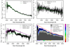 |
Fig. 5. Spectral modeling of SN 2021ckj. Top left panel: comparison of our best model (green) to the observed +7.7 day spectrum (black). Top right panel: Model spectrum (green) comparison to the +12.1 day spectrum (black). Bottom left panel: TARDIS models (green for model 1 and purple for model 2) compared to the +21.2 day spectrum (black). Bottom right panel: +7.7 day spectrum Spectral element DEComposition (SDEC) plot showing the contributions of each chemical species to the synthetic spectrum. |
Density profile parameters and velocity ranges in the TARDIS models of SN 2021ckj.
Relative mass fractions for the SN 2021ckj ejecta as constrained by the +7.7 day spectrum.
The second spectrum (Phase +12.1 days) is noisy and cannot be used to place constraints on the model composition or velocity. We included this spectrum in our modeling just to constrain the model temperature (∼8500 K) at this epoch.
The final spectrum of SN 2021ckj at +21.2 days shows P-Cygni features at ∼4000 Å and ∼8600 Å, which are produced by the Ca H&K lines and the Ca II near-infrared triplet, respectively. The flux peaks in the blue wavelengths, and we suspect it is dominated by a pseudocontinuum flux due to a multitude of Fe lines. In other Type Icn SNe, the presence of this Fe bump has been taken as evidence of a strong CSM interaction and is thought to be driven by winds or shocked gas (Perley et al. 2022). TARDIS cannot treat these interaction effects and we calculated two models at this epoch, model 1 with a boosted Lphot to reproduce the Fe features in the Fe bump and model 2 to fit the spectral energy distribution (SED) for wavelengths λ > 5500 Å. We measured the photospheric temperature (∼6500 K) from the model 2 fit to the SED.
We find that our model density profile is not consistent among all epochs. To produce reasonable agreement with the observed spectra, we needed to modify the density profile parameter ρ0. We used ρ0 = 3.5 × 10⁻¹² g cm−3 for the early (+7.7-day) spectrum and 2.0 × 10⁻¹³ g cm−3 for the +12.1-day and +21.2-day spectra. The spectra of SN 2021ckj show signs of a CSM interaction and the LC modeling in Sect. 4 suggests the ejecta may be aspherical. TARDIS cannot treat a CSM interaction or aspherical ejecta, so we acknowledge the limitations of our models to fully represent the ejecta of SN 2021ckj. The fact that we find an inconsistency in the density profile parameter ρ0 also suggests that single zone, homologously expanding, spherical ejecta are not what we are observing. Therefore, TARDIS can only provide line identifications of the broad spectral features, approximate composition, and constraints on the ejecta velocity. We find that our the photospheric velocity of 10 000 km s−1 is consistent with SN 2021csp and the broader population of typical Type Ic SNe, and that the composition is likely dominated by oxygen and carbon, while the iron group elements produce the strong absorption lines in the blue wavelengths.
6. Discussions
In this section, we discuss the ejecta and CSM properties of SN 2021ckj compared to the well-observed Type Icn SNe 2019hgp and 2021csp. From the similarity of the photometric properties between SNe 2021ckj and 2021csp, the properties of their ejecta and CSM should be very similar. The LC modeling suggests that SNe 2021ckj and 2021csp have two ejecta components (an aspherical high-energy component and a spherical canonical component) and a relatively spherical CSM. The spherical ejecta and the CSM components with the following parameters can explain their late-time LC evolution: Mej = 4 M⊙, EK = 4 × 1051 ergs, s = 2.9, and D′ = 5.1. Here, s and D′ are constants describing a single power-law density profile of the CSM according to ρCSM = Dr−s. In addition to these “canonical” components, a highly energetic component is required to explain the rapid initial decay and the photospheric expansion in the first 10 days.
On the other hand, the photometric evolution of SN 2019hgp can be explained by a spherical SN-CSM interaction model alone. There is no sign of an aspherical and energetic ejecta component. We estimate the values for the ejecta and the CSM as follows: Mej = 3 M⊙, EK = 2.5 × 1051 ergs, s = 2.9, and D′ = 2.3. The ejecta properties for SN 2019hgp are similar to those for Type Ibn SNe (Mej ∼ 2 − 6 M⊙, EK ∼ 1.0 × 1051 ergs; see Maeda & Moriya 2022).
The canonical (spherical) ejecta component of SNe 2021ckj and 2021csp are more energetic than that of SN 2019hgp. This might be related to the interpretation that SN 2021ckj (and SN 2021csp) has an aspherical energetic component in addition to a canonical one. The density distribution of the CSM is a common feature in these three SNe, and is consistent with those estimated for Type Ibn SNe (s ∼ 2.5 − 3.0; Maeda & Moriya 2022). This might imply that the mass-loss mechanism is similar in Type Icn (and also Ibn) SNe. The CSM mass of SN 2021ckj (and SN 2021csp; D′ = 5.1) is higher than that for SN 2019hgp (D′ = 2.3), even though these values are consistent with those of Type Ibn SNe (D′∼2.5 − 5.0; Maeda & Moriya 2022).
Although SNe 2021ckj and 2021csp show almost the same behavior in their photometric evolution (see Sect. 3.1), their spectral features are slightly different. As we have discussed in Sect. 3.2, the early spectrum of SN 2021ckj shows a similar ionization state of the ejecta as SN 2021csp, with a different absorption-to-emission ratio for C II lines. This implies that some aspherical structures in the emitting regions and that the viewing angles for these SNe are different. This is consistent with the conclusion inferred from the LC modeling. We might have been looking at SN 2021ckj from the polar direction of the aspherical high-energy ejecta component. Since the CSM is quickly swept up to a larger distance in the polar direction than in the other directions, we have less of an amount of CSM along the line of sight. On the other hand, the viewing angle for SN 2021csp might have been relatively off-axis, where there is a larger amount of CSM above the interaction shock due to the slower propagation of the CSM interaction shock, creating the stronger absorption parts.
The difference in the late-phase spectra of SNe 2021ckj and 2021csp might also support this scenario. Their late-time spectra share an overall similarity: a smooth continuum plus a Fe bump. However, only the spectrum of 2021csp shows clear line features. If the composition of their ejecta is the same, which is also supported by the similar set of lines in the early spectra, the diversity in the above observable is likely due to a difference in the velocity: higher velocity in SN 2021ckj and lower velocity in SN 2021csp. This can be naturally explained by the above scenario as the ejecta in the polar direction (SN 2021ckj) are faster than in an off-axis direction (SN 2021csp).
Therefore, taking the similarities and differences in their photometric and spectroscopic properties into account, we might be able to understand SNe 2021ckj and 2021csp as follows. They have similar properties as the SN ejecta, CSM, and the interaction including an aspherical explosion geometry, but involving different viewing angles. On the other hand, SN 2019hgp has different properties of the ejecta and CSM from those of SNe 2021ckj and 2021csp.
As mentioned in the introduction, there are several proposed scenarios for the progenitors of Type Icn SNe. The present work provides a new and strong constraint on the nature of the progenitor and explosion: the presence of a high-energy component in the ejecta, which requires the formation of a jet or a collimated outflow. From this point of view, the progenitors of Type Icn SNe would be more consistent with the following scenarios among those presented in Sect. 1: a merger of a WR star and a compact object, or a failed partial explosion of a WR star. In the former case, we expect an enormous diversity in their observational properties that originated from the different values of the parameters, such as the different masses of WR stars and companion stars, and different impact parameters. Thus, it might be statistically difficult to have very similar twins (SNe 2021ckj and 2021csp) in only three well-observed Type Icn SNe in the current sample. The latter scenario, which predicts a subrelativistic jet, might explain the observed properties of Type Icn SNe, even though there are many uncertain processes, such as the jet launch mechanism and the fallback processes. For a better understanding their progenitors, it is important to study the properties of the ejecta and CSM of Type Icn SNe with a larger SN sample.
7. Conclusions
We have presented photometric and spectroscopic observations of the Type Icn SN 2021ckj. Its photometric and spectroscopic properties are almost identical to those of SN 2021csp. The photometric evolution is characterized by a high peak brightness (∼ − 20 mag in the optical bands) and a rapid evolution (rise and above half-maximum times being ∼4 and ∼10 days, respectively, in the g and cyan bands). The early spectrum of SN 2021ckj shows narrow emission lines from highly ionized carbon and oxygen lines, while the late-time spectrum is smooth and featureless, except for the Ca II triplet line and the iron bump.
The TARDIS modeling of the spectra of SN 2021ckj has clarified that the composition of the SN ejecta is dominated by oxygen and carbon with the iron group elements and the photosperic velocity around the peak is ∼10 000 km s−1. The modeling has also implied the need for aspherical SN ejecta.
From the LC modeling, we have found that the ejecta and CSM properties are diverse in Type Icn SNe 2019hgp, 2021csp, and 2021ckj. The estimated ejecta properties are as follows: SNe 2021ckj and 2021csp must have two components (an aspherical high-energy component and a spherical standard-energy component) with a roughly spherical CSM. On the other hand, SN 2019hgp can be explained by a spherical SN-CSM interaction. In addition, the ejecta of SNe 2021ckj and 2021csp have a larger energy per ejecta mass than SN 2019hgp. These three SNe share a common CSM density distribution, which is similar to those of Type Ibn SNe. As for the CSM mass, SNe 2021ckj and 2021csp have higher masses than SN 2019hgp, even though both values are within the diversity range of Type Ibn SNe.
The similarities and differences of the observational properties of SNe 2021csp and 2021ckj can be explained by the viewing angle effects of an interaction between aspherical ejecta (a collimated high-energy outflow and canonical SN ejecta) and a spherical CSM. We suggest that SN 2021ckj is observed from a direction close to the jet pole, while SN 2021csp is observed from an off-axis direction.
Acknowledgments
The authors thank Avishay Gal-Yam and Morgan Fraser for providing the observational data of SNe 2019hgp and 2021csp, and Masaomi Tanaka and Jian Jiang for useful discussions. This work is based on observations collected at the European Southern Observatory under ESO program IDs 105.20DF (PI: Kuncarayakti) and 1103.D-0328, 106.216C, 108.220C (PI: Inserra; as part of ePESSTO+, the advanced Public ESO Spectroscopic Survey for Transient Objects Survey). This research made use of TARDIS, a community-developed software package for spectral synthesis in supernovae (Kerzendorf & Sim 2014; Kerzendorf et al. 2022). The development of TARDIS received support from GitHub, the Google Summer of Code initiative, and from ESA’s Summer of Code in Space program. TARDIS is a fiscally sponsored project of NumFOCUS. TARDIS makes extensive use of Astropy and Pyne. This research has made use of the NASA/IPAC Infrared Science Archive, which is funded by the National Aeronautics and Space Administration and operated by the California Institute of Technology. T.N. and H.K. are funded by the Academy of Finland projects 324504 and 328898. T.N. acknowledges the financial support by the mobility program of the Finnish Center for Astronomy with ESO (FINCA). K.M. acknowledges support from the Japan Society for the Promotion of Science (JSPS) KAKENHI grant JP18H05223, JP20H00174, and JP20H04737. The work is partly supported by the JSPS Open Partnership Bilateral Joint Research Projects between Japan and Finland (K.M. and H.K.; JPJSBP120229923). A.P., L.T. are supported by the PRIN-INAF 2022 project “Shedding light on the nature of gap transients: from the observations to the models”. S.M. acknowledges support from the Academy of Finland project 350458. K.U. acknowledges financial support from Grant-in-Aid for the Japan Society for the Promotion of Science (JSPS) Fellows (22J22705). K.U. also acknowledges financial support from AY2022 DoGS Overseas Travel Support, Kyoto University. This work was funded by ANID, Millennium Science Initiative, ICN12_009. M.G. is supported by the EU Horizon 2020 research and innovation programme under grant agreement No 101004719. T.E.M.B. acknowledges financial support from the Spanish Ministerio de Ciencia e Innovación (MCIN), the Agencia Estatal de Investigación (AEI) 10.13039/501100011033 under the PID2020-115253GA-I00 HOSTFLOWS project, from Centro Superior de Investigaciones Científicas (CSIC) under the PIE project 20215AT016 and the I-LINK 2021 LINKA20409, and the program Unidad de Excelencia María de Maeztu CEX2020-001058-M. A.R. acknowledges support from ANID BECAS/DOCTORADO NACIONAL 21202412. L.G. acknowledges financial support from the Spanish Ministerio de Ciencia e Innovación (MCIN), the Agencia Estatal de Investigación (AEI) 10.13039/501100011033, and the European Social Fund (ESF) “Investing in your future” under the 2019 Ramón y Cajal program RYC2019-027683-I and the PID2020-115253GA-I00 HOSTFLOWS project, from Centro Superior de Investigaciones Científicas (CSIC) under the PIE project 20215AT016, and the program Unidad de Excelencia María de Maeztu CEX2020-001058-M.
References
- Appenzeller, I., Fricke, K., Fürtig, W., et al. 1998, The Messenger, 94, 1 [NASA ADS] [Google Scholar]
- Arnett, W. D. 1980, ApJ, 237, 541 [Google Scholar]
- Arnett, W. D. 1982, ApJ, 253, 785 [Google Scholar]
- Bellm, E. C., Kulkarni, S. R., Graham, M. J., et al. 2019, PASP, 131, 018002 [Google Scholar]
- Cano, Z., Bersier, D., Guidorzi, C., et al. 2011, ApJ, 740, 41 [Google Scholar]
- Cardelli, J. A., Clayton, G. C., & Mathis, J. S. 1989, ApJ, 345, 245 [Google Scholar]
- Chambers, K. C., Magnier, E. A., Metcalfe, N., et al. 2016, ArXiv e-prints [arXiv:1612.05560] [Google Scholar]
- Chonis, T. S., & Gaskell, C. M. 2008, AJ, 135, 264 [NASA ADS] [CrossRef] [Google Scholar]
- Davis, K. W., Taggart, K., Tinyanont, S., et al. 2022, MNRAS, submitted [arXiv:2211.05134] [Google Scholar]
- De, K., Kasliwal, M. M., Ofek, E. O., et al. 2018, Science, 362, 201 [CrossRef] [Google Scholar]
- Drout, M. R., Soderberg, A. M., Gal-Yam, A., et al. 2011, ApJ, 741, 97 [NASA ADS] [CrossRef] [Google Scholar]
- Förster, F., Cabrera-Vives, G., Castillo-Navarrete, E., et al. 2021, AJ, 161, 242 [CrossRef] [Google Scholar]
- Fox, O. D., Silverman, J. M., Filippenko, A. V., et al. 2015, MNRAS, 447, 772 [NASA ADS] [CrossRef] [Google Scholar]
- Fraser, M., Stritzinger, M. D., Brennan, S. J., et al. 2021, ArXiv e-prints [arXiv:2108.07278] [Google Scholar]
- Freudling, W., Romaniello, M., Bramich, D. M., et al. 2013, A&A, 559, A96 [NASA ADS] [CrossRef] [EDP Sciences] [Google Scholar]
- Gal-Yam, A., Bruch, R., Schulze, S., et al. 2022, Nature, 601, 201 [NASA ADS] [CrossRef] [Google Scholar]
- Gillanders, J. H., Sim, S. A., & Smartt, S. J. 2020, MNRAS, 497, 246 [NASA ADS] [CrossRef] [Google Scholar]
- Hosseinzadeh, G., Arcavi, I., Valenti, S., et al. 2017, ApJ, 836, 158 [Google Scholar]
- Kerzendorf, W. E., & Sim, S. A. 2014, MNRAS, 440, 387 [NASA ADS] [CrossRef] [Google Scholar]
- Kerzendorf, W., Sim, S., Vogl, C., et al. 2022, https://doi.org/10.5281/zenodo.6662839 [Google Scholar]
- Kool, E. C., Karamehmetoglu, E., Sollerman, J., et al. 2021, A&A, 652, A136 [NASA ADS] [CrossRef] [EDP Sciences] [Google Scholar]
- Kuncarayakti, H., Maeda, K., Ashall, C. J., et al. 2018, ApJ, 854, L14 [NASA ADS] [CrossRef] [Google Scholar]
- Kuncarayakti, H., Maeda, K., Dessart, L., et al. 2022, ApJ, 941, L32 [NASA ADS] [CrossRef] [Google Scholar]
- Maeda, K., & Moriya, T. J. 2022, ApJ, 927, 25 [NASA ADS] [CrossRef] [Google Scholar]
- Maeda, K., Jiang, J.-A., Shigeyama, T., & Doi, M. 2018, ApJ, 861, 78 [NASA ADS] [CrossRef] [Google Scholar]
- Metzger, B. D. 2022, ApJ, 932, 84 [NASA ADS] [CrossRef] [Google Scholar]
- Pastorello, A., Wang, X. F., Ciabattari, F., et al. 2016, MNRAS, 456, 853 [Google Scholar]
- Pastorello, A., Vogl, C., Taubenberger, S., et al. 2021, TNS AstroNote, 71, 1 [NASA ADS] [Google Scholar]
- Pellegrino, C., Howell, D. A., Terreran, G., et al. 2022, ApJ, 938, 73 [NASA ADS] [CrossRef] [Google Scholar]
- Perley, D. A., Sollerman, J., Schulze, S., et al. 2022, ApJ, 927, 180 [NASA ADS] [CrossRef] [Google Scholar]
- Reguitti, A., Pastorello, A., Pignata, G., et al. 2022, A&A, 662, L10 [NASA ADS] [CrossRef] [EDP Sciences] [Google Scholar]
- Sawada, R., Kashiyama, K., & Suwa, Y. 2022, ApJ, 927, 223 [NASA ADS] [CrossRef] [Google Scholar]
- Schlafly, E. F., & Finkbeiner, D. P. 2011, ApJ, 737, 103 [Google Scholar]
- Smartt, S. J., Valenti, S., Fraser, M., et al. 2015, A&A, 579, A40 [NASA ADS] [CrossRef] [EDP Sciences] [Google Scholar]
- Smith, K. W., Smartt, S. J., Young, D. R., et al. 2020, PASP, 132, 085002 [Google Scholar]
- Tody, D. 1986, in Instrumentation in Astronomy VI, ed. D. L. Crawford, SPIE Conf. Ser., 627, 733 [NASA ADS] [CrossRef] [Google Scholar]
- Tody, D. 1993, ASP Conf. Ser., 52, 173 [NASA ADS] [Google Scholar]
- Tonry, J. L., Denneau, L., Heinze, A. N., et al. 2018, PASP, 130, 064505P [CrossRef] [Google Scholar]
- Turatto, M., Cappellaro, E., Danziger, I. J., et al. 1993, MNRAS, 262, 128 [CrossRef] [Google Scholar]
- Uno, K., Maeda, K., Nagao, T., et al. 2023, ApJ, 944, 203 [NASA ADS] [CrossRef] [Google Scholar]
- Woosley, S. E. 2017, ApJ, 836, 244 [Google Scholar]
- Yaron, O., & Gal-Yam, A. 2012, PASP, 124, 668 [Google Scholar]
- Yoon, S.-C. 2015, PASA, 32 [CrossRef] [Google Scholar]
All Tables
Density profile parameters and velocity ranges in the TARDIS models of SN 2021ckj.
Relative mass fractions for the SN 2021ckj ejecta as constrained by the +7.7 day spectrum.
All Figures
|
Fig. 1. Optical LCs of SN 2021ckj. The data were taken with the 1.82 m Copernico Telescope (triangles), NTT (circles), ZTF (filled squares), ATLAS (inverted triangles), and Pan-STARRS (diamonds). The R-band magnitudes in the NTT data have been converted into r-band magnitudes using the relation in Chonis & Gaskell (2008). The gray and black points show the r-band LCs of SNe 2019hgp (Gal-Yam et al. 2022) and 2021csp (Fraser et al. 2021), respectively, which have been plotted using their absolute magnitudes. Limiting magnitudes are indicated with arrows. All the magnitudes have been corrected with the Galactic extinction (E(B − V) = 0.027 and 0.019 mag for SNe 2021csp and 2019hgp, respectively; Schlafly & Finkbeiner 2011). The error bars for all data points have also been plotted, even though they are smaller than the sizes of the symbols in most cases. |
| In the text | |
|
Fig. 2. Evolution of the photospheric parameters estimated from blackbody fitting to the photometry of SN 2021ckj (red points connected with a line). Open red circles are the assumed values. Comparison objects, SNe 2019hgp and 2021csp, are shown with the gray and black points connected with lines, respectively. The values for the comparison objects have been taken from Gal-Yam et al. (2022) and Fraser et al. (2021). |
| In the text | |
|
Fig. 3. Spectral evolution of SN 2021ckj. Top panel: early spectra of SN 2021ckj (red), compared with the other Type Icn SNe 2019hgp (gray) and 2021csp (black). Bottom panel: same as the top panel, but for the late-time spectra. For comparison, the spectra of SNe 2020bqj (Ibn; Kool et al. 2021), 2020uem (IIn/Ia-CSM; Uno et al. 2023), and 2021foa (IIn; Reguitti et al. 2022) are plotted. These data were obtained through WISeREP (https://www.wiserep.org/object/17712). |
| In the text | |
|
Fig. 4. LC models (left panel) and evolution of the radius at the contact discontinuity, as compared to the photospheric radius (right panel). The model parameters are as follows: Mej = 3M⊙, EK = 2.5 × 1051 ergs, s = 2.9, and D′ = 2.3 for SN 2019hgp (blue lines), and Mej = 4 M⊙, EK = 4 × 1051 ergs, s = 2.9, and D′ = 5.1 for SNe 2021ckj and 2021csp (red lines). Additionally, two scenarios for the initial decay seen in SN 2021csp are shown: (1) the SN-CSM interaction driven by a highly energetic component (magenta lines) and (2) the shock-cooling of an energetic component (solid cyan lines). As a comparison, the same is also shown, but for a canonical explosion energy (dashed-cyan line). The gray hatching shows the template of the LCs of Type Ibn SNe (Hosseinzadeh et al. 2017; Maeda & Moriya 2022). |
| In the text | |
|
Fig. 5. Spectral modeling of SN 2021ckj. Top left panel: comparison of our best model (green) to the observed +7.7 day spectrum (black). Top right panel: Model spectrum (green) comparison to the +12.1 day spectrum (black). Bottom left panel: TARDIS models (green for model 1 and purple for model 2) compared to the +21.2 day spectrum (black). Bottom right panel: +7.7 day spectrum Spectral element DEComposition (SDEC) plot showing the contributions of each chemical species to the synthetic spectrum. |
| In the text | |
Current usage metrics show cumulative count of Article Views (full-text article views including HTML views, PDF and ePub downloads, according to the available data) and Abstracts Views on Vision4Press platform.
Data correspond to usage on the plateform after 2015. The current usage metrics is available 48-96 hours after online publication and is updated daily on week days.
Initial download of the metrics may take a while.