| Issue |
A&A
Volume 672, April 2023
|
|
|---|---|---|
| Article Number | L3 | |
| Number of page(s) | 7 | |
| Section | Letters to the Editor | |
| DOI | https://doi.org/10.1051/0004-6361/202346072 | |
| Published online | 29 March 2023 | |
Letter to the Editor
Analytic characterization of sub-Alfvénic turbulence energetics
1
Owens Valley Radio Observatory, California Institute of Technology, MC 249-17, Pasadena, CA 91125, USA
e-mail: This email address is being protected from spambots. You need JavaScript enabled to view it.
2
Department of Physics & ITCP, University of Crete, 70013 Heraklion, Greece
3
Institute of Astrophysics, Foundation for Research and Technology-Hellas, Vasilika Vouton, 70013 Heraklion, Greece
Received:
3
February
2023
Accepted:
21
February
2023
Abstract
Magnetohydrodynamic (MHD) turbulence is a cross-field process relevant to many systems. A prerequisite for understanding these systems is to constrain the role of MHD turbulence, and in particular, the energy exchange between kinetic and magnetic forms. The energetics of strongly magnetized and compressible turbulence has so far resisted attempts to understand them. Numerical simulations reveal that kinetic energy can be orders of magnitude higher than fluctuating magnetic energy. We solved this lack-of-balance puzzle by calculating the energetics of compressible and sub-Alfvénic turbulence based on the dynamics of coherent cylindrical fluid parcels. Using the MHD Lagrangian, we proved analytically that the bulk of the magnetic energy transferred to kinetic energy is the energy that is stored in the coupling between the ordered and fluctuating magnetic field. The analytical relations are in strikingly good agreement with numerical data, up to second-order terms.
Key words: magnetic fields / magnetohydrodynamics (MHD) / plasmas / methods: analytical / turbulence
© The Authors 2023
 Open Access article, published by EDP Sciences, under the terms of the Creative Commons Attribution License (https://creativecommons.org/licenses/by/4.0), which permits unrestricted use, distribution, and reproduction in any medium, provided the original work is properly cited.
This article is published in open access under the Subscribe to Open model. This email address is being protected from spambots. You need JavaScript enabled to view it. to support open access publication.
1. Introduction
Magnetohydrodynamic (MHD) turbulence is involved in a plethora of physical phenomena (Biskamp 2003; Beresnyak 2019; Matthaeus & Velli 2011; Matthaeus 2021; Schekochihin 2020). The interplay between kinetic and magnetic energy is important for understanding these processes (Goldstein et al. 1995; Ciolek & Basu 2006; Kirk et al. 2009; Oughton et al. 2013; Matthaeus et al. 1983; Zweibel & McKee 1995); Schekochihin et al. 2007; Cho & Lazarian 2002; Federrath et al. 2011. It is challenging to understand the energy exchange between kinetic and magnetic forms because the MHD equations are nonlinear. For this reason, several assumptions and approximations are usually employed.
A widely employed approximation is the incompressibility of the gas (Sridhar & Goldreich 1994; Goldreich & Sridhar 1995), although this is only applicable to a limited number of systems. Compressible MHD turbulence is more complex, and additional energy terms contribute to the energy cascade. One main difference in the energy cascade rate of incompressible and compressible turbulence is that in the latter, the background magnetic field (B0) appears with leading-order terms (Banerjee & Galtier 2013; Andrés & Sahraoui 2017). In contrast, the incompressible turbulence energy cascade is dominated by the increments of the magnetic and velocity fluctuations, and B0 only appears in higher-order statistics (Wan et al. 2012). This result motivated the hypothesis that B0 might also appear in the total (kinetic and magnetic) fluctuating energy of compressible MHD turbulence (Andrés & Sahraoui 2017), whereas in incompressible turbulence, the total fluctuating energy is dominated by the fluctuating (second-order) kinetic and magnetic energy.
In incompressible and sub-Alfvénic turbulence, the fluctuating magnetic energy is completely transferred to kinetic energy, and the volume-averaged quantities are in equilibrium, ρ⟨u2⟩/2 ∼ ⟨δB2⟩/8π, when turbulence is maintained in a steady state. In contrast, direct numerical simulations of sub-Alfvénic and compressible turbulence show that the volume-averaged kinetic energy is much higher than the second-order fluctuating magnetic energy, ρ⟨u2⟩/2 ≫ ⟨δB2⟩/8π (Heitsch et al. 2001; Li et al. 2012a,b), and their relative ratio depends on the amplitude of B0 (Andrés et al. 2018; Lim et al. 2020; Skalidis et al. 2021; Beattie et al. 2022b). The excess of the kinetic energy suggests that B0 might provide additional energy to the fluid.
The role of B0 in the energetics can be intuitively understood when we decompose the total magnetic field into a background and a fluctuating component. In incompressible turbulence, the fluctuating magnetic energy comes only from the perturbations of the magnetic field, which are of second order. However, in compressible turbulence, the background field appears in the total fluctuating magnetic energy due to the coupling between the background field and magnetic perturbations (δB). The magnetic coupling, expressed as B0 ⋅ δB, can only be realized in compressible turbulence (Montgomery et al. 1987; Bhattacharjee & Hameiri 1988; Bhattacharjee et al. 1998; Fujimura & Tsuneta 2009) and is the dominant (first-order) term of the fluctuating magnetic energy.
In sub-Alfvénic and compressible turbulence, numerical data show that B0 ⋅ δB stores most of the magnetic energy, and that the kinetic energy approximately reaches equipartition with the fluctuations of the coupling term (Skalidis & Tassis 2021; Skalidis et al. 2021; Beattie et al. 2022a,b). Thus, the magnetic coupling holds the key for understanding the energetics of strongly magnetized and compressible turbulence. However, there is still a lack of first-principle understanding of the role of B0 ⋅ δB in MHD turbulence dynamics and how it contributes to the averaged energetics.
We present an analytical theory of the role of the coupling potential in the energy exchange of sub-Alfvénic and compressible turbulence, which is encountered in systems such as tokamaks (Strauss 1976, 1977; Zocco & Schekochihin 2011), in the interstellar medium (Mouschovias et al. 2006; Panopoulou et al. 2015, 2016; Planck Collaboration Int. XXXV 2016; Skalidis et al. 2022), and the Sun (Verdini & Velli 2007; Tenerani & Velli 2017; Kasper et al. 2021; Zank et al. 2022). We write the Lagrangian of coherent flux structures (Crowley et al. 2022), which allows us to approximate turbulence properties in a deterministic manner, and calculate analytically the energy exchange between kinetic and magnetic forms as a function of the Alfvénic Mach number (ℳA). We find remarkable agreement between the analytically calculated energetics and numerical data. We conclude that the majority of the fluctuating magnetic energy transferred to kinetic energy is provided by the coupling between the background and the fluctuating magnetic field.
2. Model
We considered a turbulent fluid characterized by the commonly employed properties: (1) spatial homogeneity, (2) infinite magnetic and kinetic Reynolds number, and (3) time stationarity. We considered that the fluid consists of coherent flux tubes (e.g., Fig. 1 in Banerjee & Galtier 2013) (or fluid parcels) with coordinates (r(t),ϕ(t),z(t)), as shown in Fig. 1. Cylindrical coordinates are motivated by studies showing that the properties of strongly magnetized turbulence are axially symmetric, with B0 being the axis of symmetry (Goldreich & Sridhar 1995; Maron & Goldreich 2001). We assumed the following initial conditions: (1) uniform temperature, (2) uniform density, (3) no bulk velocity, (4) uniform static magnetic field ( ), and (5) no self-gravity. We henceforth adopt the following notation: z = ℓ∥ and r = ℓ⊥, where ℓ∥ and ℓ⊥ denote parcel sizes parallel and perpendicular to B0, respectively.
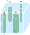 |
Fig. 1. Magnetized fluid consisting of multiple coherent cylindrical fluid parcels. Red arrows show the initial magnetic field morphology. Untwisted fluid parcels are elongated, ℓ∥ ≫ ℓ⊥, and their motion is longitudinal along or perpendicular to B0. In sub-Alfvénic turbulence, the motion of these fluid parcels can be decomposed into two independent velocity components, parallel (black arrows) and perpendicular (orange arrows) to B0. |
We perturbed the magnetic field of a coherent fluid structure with a length scale  by δBℓ such that |B0|≫|δBℓ|, which applies to sub-Alfvénic turbulence. Magnetic perturbations tend to redistribute the magnetic flux within a fluid. For ideal-MHD (flux-freezing) conditions, the magnetic flux is preserved. Thus, the surface of the perturbed fluid parcel (Sℓ) follows the magnetic field lines. The motion of the field lines, and hence of Sℓ, can be either parallel or perpendicular to B0 (Fig. 1): (1) Squeezing and stretching of Sℓ along B0 leads to parallel motions,
  . (2) Fluctuations of ℓ⊥ lead to perpendicular motions,
  . Finally, (3) twisting leads to rotational motions,
  . This naturally defines ℓ∥ and ℓ⊥ as the coherence lengths of the perturbed volume parallel and perpendicular to B0, respectively. We focused on large scales since coherent structures are prominent there (De Giorgio et al. 2017). We invoke as a boundary condition a local environment beyond ℓ (pressure wall).
The flux freezing theorem is
 (1)
(1)
The cross section of the coherent volume perpendicular and parallel to B0 is  , and
, and  , respectively. The cross section related to the rotational motion is
  . The total magnetic field in cylindrical coordinates can be expressed as
  . From Eq. (1), we obtain that when |B0|≫|δB|, magnetic perturbations along S∥, ℓ are associated with a longitudinal motion such that
 (2)
(2)
where we have considered that the initial dimension of the perturbed volume ℓ⊥, 0 is much larger than its perturbations. Along S⊥, ℓ, we find that
 (3)
(3)
while the azimuthal velocity along Sϕ, ℓ is
 (4)
(4)
As a result of assuming |B0|≫|δB|, we have obtained that parallel and perpendicular motions are decoupled. The coupling of parallel and perpendicular motions becomes inevitable when |B0|∼|δB| (Eq. (3)).
In sub-Alfvénic turbulence, magnetic tension dominates magnetic pressure (Passot & Vázquez-Semadeni 2003). The high tension suppresses transverse oscillations due to the strong restoring torques. Thus, twisting would have minimum contribution to the dynamics (e.g., Longcope & Klapper 1997) and motions would be mostly longitudinal ( ). Since u⊥ϕ, ℓ → 0, then due to Eqs. (3) and (4), ℓ∥ ≫ ℓ⊥, which implies that untwisted coherent structures are stretched toward the B0 axis, which is consistent with the anisotropic properties of sub-Alfvénic turbulence (Shebalin et al. 1983; Higdon 1984; Oughton et al. 1994, 2013; Sridhar & Goldreich 1994; Goldreich & Sridhar 1995; Oughton & Matthaeus 2020; Cho & Lazarian 2003; Yang et al. 2018; Makwana & Yan 2020; Gan et al. 2022).
For untwisted fluid parcels, the perpendicular component of the magnetic fluctuations has a dominant radial component such that δB⊥, ℓ ≈ δB⊥r, ℓ. From Eqs. (2) and (3), we derive
 (5)
(5)
 (6)
(6)
The difference in the scaling is due to the Lorenz force by B0, which affects perpendicular motions, while it has no effect on parallel motions.
3. MHD Lagrangian of coherent structures
We write the Lagrangian for the perturbed volume. We place the reference frame at the center of mass of the target volume, hence there is no bulk velocity term in the Lagrangian. Therefore, all the velocity components are due to internal motions induced by magnetic perturbations. We focus on low plasma-beta fluids1, which for sub-Alfvénic turbulence corresponds to high sonic Mach numbers (ℳs). The perturbed Lagrangian (Newcomb 1962; Andreussi et al. 2016; Kulsrud 2005) of the coherent cylindrical fluid parcel, with surface Sℓ, can be split into a parallel and a perpendicular term (Appendix A),
 (7)
(7)
Due to Eqs. (2) and (3), δB∥, ℓ, and δB⊥, ℓ are generalized coordinates of δℒ and ℓ∥(t) = C/δB⊥, ℓ(t) (Eq. (6)), where C is a constant determined from the initial conditions. With this expression, we eliminate ℓ∥ from the Lagrangian, which up to second-order terms is separable into a parallel and a perpendicular part, and is analytically solvable,
 (8)
(8)
 (9)
(9)
We solve the Euler-Lagrange equations for δℒ∥ (Appendix B) and δℒ⊥ (Appendix C) and derive the analytical solutions of the velocity (u∥, ℓ(t), u⊥, ℓ(t)) and magnetic fluctuations (δB∥, ℓ(t), δB⊥, ℓ(t)) of Sℓ. We find that δB∥, ℓ ∼ t2, u⊥, ℓ ∼ t, and δB⊥, ℓ ∼ t−1, while u∥, ℓ is set by the initial conditions (free streaming of the gas). We used these analytical solutions in order to calculate the averaged energetics of a strongly magnetized and compressible fluid.
4. Energetics
The total energy of fully developed turbulence is stationary because energy diffusion is balanced by injection. Time stationarity enables us to approximate turbulence energetics with the leading-order solutions that we obtained because our approximations preserve time symmetry, and thus energy is conserved. The statistical properties of large-scale coherent structures accurately approximate the volume-averaged turbulent statistical properties. Thus, for an ergodic fluid (Monin & I’Aglom 1971; Galanti & Tsinober 2004), averaging the turbulent statistical properties over the volume of the fluid at a given time step (⟨f⟩𝒱=∫𝒱f) is approximately equivalent to averaging over multiple realizations of a typical large-scale coherent structure (⟨fℓ⟩𝒯=∫𝒯fℓ), hence ⟨f⟩𝒱 ∼ ⟨fℓ⟩𝒯, where f denotes an energy term, and 𝒯 corresponds to the coherent structure crossing time. We next analytically compute the ⟨fℓ⟩𝒯 energy contribution of each Lagrangian term (Eq. (7)) and their relative ratios. Since coherent cylindrical parcels are characterized by two different coherence lengths ℓ∥ and ℓ⊥, they also have two different crossing times: 𝒯∥ and 𝒯⊥, respectively. We compare the ⟨fℓ⟩𝒯 analytical energy ratios with the ⟨f⟩𝒱 numerical values. The numerical results correspond to simulations of ideal isothermal MHD turbulence without self-gravity, and turbulence is maintained in a quasi-static state by injecting energy with an external forcing mechanism (Beattie et al. 2022b). These simulation are forced with a mixture of compressible and incompressible modes, but the driving modes do not affect the energetics of sub-Alfvénic and compressible turbulence (Skalidis et al. 2021).
4.1. Kinetic energy
The total averaged kinetic energy (Ekinetic) of the coherent fluid parcel with scale ℓ is
 (10)
(10)
The kinetic energy is dominated to first order by u⊥, ℓ. Thus, the average Alfvénic Mach number to first order is
 (11)
(11)
4.2. Harmonic potential
From Eqs. (B.3) and (C.2), we find that  , and
, and  . The total time-averaged harmonic potential energy (Eharmonic) density is equal to
 (12)
(12)
where ζ = δB⊥, max/δB∥, max. Sub-Alfvénic turbulence is anisotropic (Shebalin et al. 1983; Higdon 1984; Oughton et al. 1994; Goldreich & Sridhar 1995), with the anisotropy between δB⊥ and δB∥ depending on ℳA (Beattie et al. 2020). To account for this property, we assumed that ζ is a function of ℳA. When ℳA → 0, B0 suppresses any bending of the magnetic field lines with the amplitude of δB∥ being larger than that of δB⊥ (Beattie et al. 2020), hence ζ → 0; this is also a consequence of ∇ ⋅ B = 0 for anisotropic fluid parcels with ℓ∥ ≫ ℓ⊥. For ℳA → 1, fluctuations tend to become more isotropic, and hence  . These limiting behaviors are consistent with numerical simulations (Beattie et al. 2020, 2022b).
4.3. Coupling potential
According to Eq. (10), B0 ⋅ δB contributes to Ekinetic since
 (13)
(13)
to first order. This equation demonstrates that the energy stored in the coupling potential is in equipartition with the averaged kinetic energy when turbulence is sub-Alfvénic.
4.4. Energetics ratios
The Ekinetic/Ecoupling ratio is
 (14)
(14)
For ℳA → 0, Ecoupling ≈ Ekinetic, while for ℳA → 1, Ekinetic ≳ Ecoupling. Ekinetic becomes higher than Ecoupling because u∥, ℓ contributes more to Ekinetic as ℳA increases. When ℳA → 1,  , so that the Ekinetic/Ecoupling ratio in trans-Alfvénic turbulence scales as
 (15)
(15)
Regarding the Eharmonic/Ecoupling ratio, we find that
 (16)
(16)
which for the two limiting cases of ζ (ℳA) becomes
 (17)
(17)
4.5. Comparison between analytical and numerical results
In Fig. 2 we compare the analytically calculated energy ratios with numerical results from the literature (Beattie et al. 2022b). The lines correspond to the analytical relations for Eharmonic/Ecoupling (Eq. (17)) and Ekinetic/Eharmonic (Eq. (15)), while the colored points correspond to the numerical values. The numerical data behave as predicted by the analytical relations. The scatter of triangles increases at higher ℳA because thermal pressure starts becoming important there, and hence the contribution of thermal motions to the kinetic energy increases. In the limit of ℳA ≪ 1, thermal pressure is subdominant and β → 0. For ℳA = 1, we obtain that β → 0 when ℳs ≫ 1, while when ℳs ≲ 1, β → 1. Thus, for trans-Alvfénic turbulence, thermal pressure becomes important only for low ℳs, while at high ℳs, it has a minor contribution to the energetics. In our calculations, we neglected thermal pressure, and for this reason, at ℳA = 1, triangles are consistent with the analytical ratio of Ekinetic/Ecoupling (blue line) when ℳs ≥ 2, while at lower ℳs, the deviation between numerical and analytical results increases because β, hence the relative contribution of thermal pressure, increases. For ℳA < 1, β ≪ 1, and for this reason, the numerical data agree perfectly with the analytical ratio (blue line). Finally, when we account for the contribution from both B0 ⋅ δB and δB2, the total energy stored in magnetic fluctuations (Em, total=Ecoupling+Eharmonic) is very close to equipartition with kinetic energy, as shown by the red boxes.
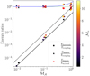 |
Fig. 2. Comparison between analytical and numerical results. The solid and dashed thick black lines correspond to the Eharmonic/Ecoupling ratio obtained analytically for ℳA → 0 (ζ = 0) and ℳA → 1 ( |

5. Discussion and conclusions
Analytical calculations of strongly magnetized and compressible (isothermal) turbulence show that B0 appears in the energy cascade with leading-order terms (Banerjee & Galtier 2013; Andrés et al. 2018). This is in striking contrast to incompressible turbulence, where B0 appears in higher-order terms (Wan et al. 2012). In the formalism presented here, the incompressible limit is approximated when B0 ⋅ δB = 0. In this case, B0 does not appear in the dominant Lagrangian terms, hence the averaged kinetic energy would scale linearly with the fluctuating magnetic energy, δuℓ ∼ δBℓ (or equivalently, ℳA ∼ δBℓ). However, in agreement with previous works (Wan et al. 2012), our formalism shows that B0 appears in the energetics of incompressible turbulence because of the coupling between δB∥, ℓ and δB⊥, ℓ (Eq. (3)) when higher-order terms are considered.
For sub-Alfvénic and compressible turbulence, we find that B0 ⋅ δB is the leading term in the dynamics, and as a result, the scaling between velocity and magnetic fluctuations becomes  , or equivalently,
  , which is supported by numerical data (Beattie et al. 2020). In compressible and strongly magnetized turbulence, compression and dilatation of the gas locally changes the energy cascade rate (Banerjee & Galtier 2013). These local energy fluctuations can only be realized in compressible turbulence and might be related to the fluctuations of the B0 ⋅ δB potential. Our analytical results prove that the total averaged magnetic energy transferred to kinetic is equal to
  .
.
The consistency between our analytical relations and numerical data is remarkable. It is not the first time that simple analytical arguments agree quantitatively with numerical simulations of nonlinear problems (e.g., Mouschovias et al. 2011). However, an analytical theory is always advantageous because it allows us to achieve a deeper understanding of complex problems. For this reason, the formalism we presented might offer new insights into the energetics of strongly magnetized and compressible turbulence. We hope that it motivates future works about the role of magnetic couplings in the energy cascade.
The relative ratio of the thermal and magnetic pressure is the plasma beta, which is defined as  .
.
Acknowledgments
We would like to thank the anonymous referee for reviewing our manuscript. We are grateful to T. Ch. Mouschovias, and P. F. Hopkins for stimulating discussions. We also thank E. N. Economou, V. Pelgrims, E. Ntormousi, A. Tsouros, and I. Komis for useful suggestions on the manuscript. This work was supported by NSF grant AST-2109127. We acknowledge support by the European Research Council under the European Union’s Horizon 2020 research and innovation programme, grant agreement No. 771282 (RS and KT); by the Hellenic Foundation for Research and Innovation under the “First Call for H.F.R.I. Research Projects to support Faculty members and Researchers and the procurement of high-cost research equipment grant”, Project 1552 CIRCE (VP); and from the Foundation of Research and Technology – Hellas Synergy Grants Program (project MagMASim, VP, and project POLAR, KT).
References
- Andrés, N., & Sahraoui, F. 2017, Phys. Rev. E, 96, 053205 [CrossRef] [Google Scholar]
- Andrés, N., Sahraoui, F., Galtier, S., et al. 2018, J. Plasma Phys., 84, 905840404 [CrossRef] [Google Scholar]
- Andreussi, T., Morrison, P. J., & Pegoraro, F. 2016, Phys. Plasmas, 23, 102112 [NASA ADS] [CrossRef] [Google Scholar]
- Banerjee, S., & Galtier, S. 2013, Phys. Rev. E, 87, 013019 [NASA ADS] [CrossRef] [Google Scholar]
- Basu, S., Ciolek, G. E., Dapp, W. B., & Wurster, J. 2009, New Astron., 14, 483 [NASA ADS] [CrossRef] [Google Scholar]
- Beattie, J. R., Federrath, C., & Seta, A. 2020, MNRAS, 498, 1593 [Google Scholar]
- Beattie, J. R., Krumholz, M. R., Federrath, C., Sampson, M., & Crocker, R. M. 2022a, Front. Astron. Space Sci., 9, 900900 [NASA ADS] [CrossRef] [Google Scholar]
- Beattie, J. R., Krumholz, M. R., Skalidis, R., et al. 2022b, MNRAS, 515, 5267 [NASA ADS] [CrossRef] [Google Scholar]
- Beresnyak, A. 2019, Liv. Rev. Comput. Astrophys., 5, 2 [CrossRef] [Google Scholar]
- Bhattacharjee, A., & Hameiri, E. 1988, Phys. Fluids, 31, 1153 [Google Scholar]
- Bhattacharjee, A., Ng, C. S., & Spangler, S. R. 1998, ApJ, 494, 409 [Google Scholar]
- Biskamp, D. 2003, Plasma Phys. Control. Fusion, 45, 1827 [CrossRef] [Google Scholar]
- Cho, H., Ryu, D., & Kang, H. 2022, ApJ, 926, 183 [NASA ADS] [CrossRef] [Google Scholar]
- Cho, J., & Lazarian, A. 2002, Phys. Rev. Lett., 88, 245001 [Google Scholar]
- Cho, J., & Lazarian, A. 2003, MNRAS, 345, 325 [NASA ADS] [CrossRef] [Google Scholar]
- Ciolek, G. E., & Basu, S. 2006, ApJ, 652, 442 [NASA ADS] [CrossRef] [Google Scholar]
- Colman, T., Robitaille, J.-F., Hennebelle, P., et al. 2022, MNRAS, 514, 3670 [NASA ADS] [CrossRef] [Google Scholar]
- Crowley, C. J., Pughe-Sanford, J. L., Toler, W., et al. 2022, Proc. Natl. Acad. Sci., 119, e2120665119 [CrossRef] [Google Scholar]
- De Giorgio, E., Servidio, S., & Veltri, P. 2017, Sci. Rep., 7, 13849 [NASA ADS] [CrossRef] [Google Scholar]
- Elmegreen, B. G. 2009, in The Galaxy Disk in Cosmological Context, eds. J. Andersen, B. Nordströara, & J. Bland-Hawthorn, 254, 289 [NASA ADS] [Google Scholar]
- Elmegreen, B. G., & Scalo, J. 2004, ARA&A, 42, 211 [Google Scholar]
- Eswaran, V., & Pope, S. B. 1988, Comput. Fluids, 16, 257 [NASA ADS] [CrossRef] [Google Scholar]
- Federrath, C., Chabrier, G., Schober, J., et al. 2011, Phys. Rev. Lett., 107, 114504 [NASA ADS] [CrossRef] [Google Scholar]
- Fujimura, D., & Tsuneta, S. 2009, ApJ, 702, 1443 [Google Scholar]
- Galanti, B., & Tsinober, A. 2004, Phys. Lett. A, 330, 173 [NASA ADS] [CrossRef] [Google Scholar]
- Gan, Z., Li, H., Fu, X., & Du, S. 2022, ApJ, 926, 222 [NASA ADS] [CrossRef] [Google Scholar]
- Girichidis, P., Walch, S., Naab, T., et al. 2016, MNRAS, 456, 3432 [NASA ADS] [CrossRef] [Google Scholar]
- Goldreich, P., & Sridhar, S. 1995, ApJ, 438, 763 [Google Scholar]
- Goldstein, M. L., Roberts, D. A., & Matthaeus, W. H. 1995, ARA&A, 33, 283 [NASA ADS] [CrossRef] [Google Scholar]
- Hanasoge, S. M., Hotta, H., & Sreenivasan, K. R. 2020, Sci. Adv., 6, eaba9639 [NASA ADS] [CrossRef] [Google Scholar]
- Heitsch, F., Zweibel, E. G., Mac Low, M.-M., Li, P., & Norman, M. L. 2001, ApJ, 561, 800 [Google Scholar]
- Higdon, J. C. 1984, ApJ, 285, 109 [Google Scholar]
- Iffrig, O., & Hennebelle, P. 2017, A&A, 604, A70 [NASA ADS] [CrossRef] [EDP Sciences] [Google Scholar]
- Kasper, J. C., Klein, K. G., Lichko, E., et al. 2021, Phys. Rev. Lett., 127, 255101 [NASA ADS] [CrossRef] [Google Scholar]
- Kirk, H., Johnstone, D., & Basu, S. 2009, ApJ, 699, 1433 [NASA ADS] [CrossRef] [Google Scholar]
- Klessen, R. S., & Hennebelle, P. 2010, A&A, 520, A17 [NASA ADS] [CrossRef] [Google Scholar]
- Kritsuk, A. G., Ustyugov, S. D., & Norman, M. L. 2017, New J. Phys., 19, 065003 [Google Scholar]
- Krumholz, M., & Burkert, A. 2010, ApJ, 724, 895 [NASA ADS] [CrossRef] [Google Scholar]
- Krumholz, M. R., & Burkhart, B. 2016, MNRAS, 458, 1671 [NASA ADS] [CrossRef] [Google Scholar]
- Kulsrud, R. M. 2005, Plasma Physics for Astrophysics (Princeton: Princeton University Press) [Google Scholar]
- Li, P. S., McKee, C. F., & Klein, R. I. 2012a, ApJ, 744, 73 [NASA ADS] [CrossRef] [Google Scholar]
- Li, P. S., Myers, A., & McKee, C. F. 2012b, ApJ, 760, 33 [NASA ADS] [CrossRef] [Google Scholar]
- Lim, J., Cho, J., & Yoon, H. 2020, ApJ, 893, 75 [NASA ADS] [CrossRef] [Google Scholar]
- Longcope, D. W., & Klapper, I. 1997, ApJ, 488, 443 [NASA ADS] [CrossRef] [Google Scholar]
- Mac Low, M.-M., Klessen, R. S., Burkert, A., & Smith, M. D. 1998, Phys. Rev. Lett., 80, 2754 [NASA ADS] [CrossRef] [Google Scholar]
- Makwana, K. D., & Yan, H. 2020, Phys. Rev. X, 10, 031021 [NASA ADS] [Google Scholar]
- Maron, J., & Goldreich, P. 2001, ApJ, 554, 1175 [Google Scholar]
- Matthaeus, W. H. 2021, Phys. Plasmas, 28, 032306 [NASA ADS] [CrossRef] [Google Scholar]
- Matthaeus, W. H., & Velli, M. 2011, Space Sci Rev, 160, 145 [NASA ADS] [CrossRef] [Google Scholar]
- Matthaeus, W. H., Goldstein, M. L., & Montgomery, D. C. 1983, Phys. Rev. Lett., 51, 1484 [Google Scholar]
- McKee, C. F. 1989, ApJ, 345, 782 [NASA ADS] [CrossRef] [Google Scholar]
- Monin, A. S., & I’Aglom, A. M. 1971, Statistical fluid Mechanics; Mechanics of Turbulence (Cambridge: Cambridge University Press) [Google Scholar]
- Montgomery, D., Brown, M. R., & Matthaeus, W. H. 1987, J. Geophys. Res., 92, 282 [Google Scholar]
- Mouschovias, T. C., Tassis, K., & Kunz, M. W. 2006, ApJ, 646, 1043 [Google Scholar]
- Mouschovias, T. C., Ciolek, G. E., & Morton, S. A. 2011, MNRAS, 415, 1751 [NASA ADS] [CrossRef] [Google Scholar]
- Newcomb, W. A. 1962, Nucl. Fusion Suppl. Part, 2, 451 [Google Scholar]
- Oughton, S., & Matthaeus, W. H. 2020, ApJ, 897, 37 [Google Scholar]
- Oughton, S., Priest, E. R., & Matthaeus, W. H. 1994, J. Fluid Mech., 280, 95 [NASA ADS] [CrossRef] [Google Scholar]
- Oughton, S., Wan, M., Servidio, S., & Matthaeus, W. H. 2013, ApJ, 768, 10 [NASA ADS] [CrossRef] [Google Scholar]
- Panopoulou, G., Tassis, K., Blinov, D., et al. 2015, MNRAS, 452, 715 [Google Scholar]
- Panopoulou, G. V., Psaradaki, I., & Tassis, K. 2016, MNRAS, 462, 1517 [Google Scholar]
- Park, J., & Ryu, D. 2019, ApJ, 875, 2 [NASA ADS] [CrossRef] [Google Scholar]
- Passot, T., & Vázquez-Semadeni, E. 2003, A&A, 398, 845 [NASA ADS] [CrossRef] [EDP Sciences] [Google Scholar]
- Piontek, R. A., & Ostriker, E. C. 2007, ApJ, 663, 183 [NASA ADS] [CrossRef] [Google Scholar]
- Planck Collaboration Int. XXXV. 2016, A&A, 586, A138 [NASA ADS] [CrossRef] [EDP Sciences] [Google Scholar]
- Schekochihin, A. A. 2020, ArXiv e-prints [arXiv:2010.00699] [Google Scholar]
- Schekochihin, A. A., Iskakov, A. B., Cowley, S. C., et al. 2007, New J. Phys., 9, 300 [Google Scholar]
- Shebalin, J. V. 2013, Geophys. Astrophys. Fluid Dyn., 107, 411 [NASA ADS] [CrossRef] [Google Scholar]
- Shebalin, J. V., Matthaeus, W. H., & Montgomery, D. 1983, J. Plasma Phys., 29, 525 [Google Scholar]
- Skalidis, R., & Tassis, K. 2021, A&A, 647, A186 [NASA ADS] [CrossRef] [EDP Sciences] [Google Scholar]
- Skalidis, R., Sternberg, J., Beattie, J. R., Pavlidou, V., & Tassis, K. 2021, A&A, 656, A118 [NASA ADS] [CrossRef] [EDP Sciences] [Google Scholar]
- Skalidis, R., Tassis, K., Panopoulou, G. V., et al. 2022, A&A, 665, A77 [NASA ADS] [CrossRef] [EDP Sciences] [Google Scholar]
- Sridhar, S., & Goldreich, P. 1994, ApJ, 432, 612 [Google Scholar]
- Strauss, H. R. 1976, Phys. Fluids, 19, 134 [NASA ADS] [CrossRef] [Google Scholar]
- Strauss, H. R. 1977, Phys. Fluids, 20, 1354 [NASA ADS] [CrossRef] [Google Scholar]
- Tenerani, A., & Velli, M. 2017, ApJ, 843, 26 [Google Scholar]
- Verdini, A., & Velli, M. 2007, ApJ, 662, 669 [Google Scholar]
- Wan, M., Oughton, S., Servidio, S., & Matthaeus, W. H. 2012, J. Fluid Mech., 697, 296 [NASA ADS] [CrossRef] [Google Scholar]
- Yang, L., Zhang, L., He, J., et al. 2018, ApJ, 866, 41 [NASA ADS] [CrossRef] [Google Scholar]
- Yang, Y., Wan, M., Matthaeus, W. H., & Chen, S. 2021, J. Fluid Mech., 916, A4 [NASA ADS] [CrossRef] [Google Scholar]
- Zank, G. P., Zhao, L. L., Adhikari, L., et al. 2022, ApJ, 926, L16 [NASA ADS] [CrossRef] [Google Scholar]
- Zocco, A., & Schekochihin, A. A. 2011, Phys. Plasmas, 18, 102309 [NASA ADS] [CrossRef] [Google Scholar]
- Zweibel, E. G., & McKee, C. F. 1995, ApJ, 439, 779 [NASA ADS] [CrossRef] [Google Scholar]
Appendix A: Lagrangian of coherent cylindrical parcels
We used the MHD Lagrangian as derived by Newcomb (Newcomb 1962) for isothermal magnetized fluids. The total MHD Lagrangian is the sum of the kinetic and the total potential energy of all the fluid elements within a volume 𝒱,
 (A.1)
(A.1)
where Ps is the thermal pressure, and Φ is the gravitational potential. The equation of motion for magnetized turbulent fluids is obtained from the stationary-action principle  . We focused on fluids in which magnetic pressure dominates thermal pressure (B2/8π≫Ps), and we ignored self-gravity, Φ = 0. Therefore, the dominant potential term in the Lagrangian is magnetic pressure. When we consider that the ensemble of the fluid elements moves as a coherent cylinder (Fig. 1), then the integration of the Lagrangian takes place within the volume of the cylinder. In this case, the integrated Lagrangian terms correspond to the kinetic and the magnetic energy of the cylinder. The perturbed Lagrangian of a cylinder is (using Eqs. 2, 3, and 4)
 (A.2)
(A.2)
For untwisted cylinders, all terms containing a ϕ component are zero. Then, the Lagrangian contains only the parallel and the perpendicular (longitudinal) components, which are generally coupled due to the  term. For sub-Alfvénic turbulence, this is a higher-order term because |B0| ≫ |δB|. By keeping the dominant (second-order) terms, we derived the total perturbed Lagrangian of a coherent cylindrical structure, which to leading order, can be expressed as the sum of two independent parts (parallel and perpendicular to the background magnetic field, Eqs. 8 and 9).
Appendix B: Solutions of δℒ∥
From the Euler-Lagrange equation of δℒ∥, we obtain
 (B.1)
(B.1)
where  is the Alfvénic speed.
Initially, we compressed the perturbed volume perpendicular to B0, then released it and allowed the compression to propagate. For the initial conditions, we considered that u⊥, ℓ(t = 0) = 0 and δB‖,ℓ(t = 0) = δB‖,max. We might have initiated the fluid parcel at δB‖,ℓ(t = 0) = −δB‖,max, but in that case, u⊥, ℓ(t = 0)≠0. Solutions of Eq. B.1 are harmonic, but are valid only for early times because at later times, nonlinear interactions become important and energy is diffused. Below, we consider the scenario of energy diffusing due to the shock formation because we considered highly compressible fluids. Without loss of generality, we can consider any diffusive process.
From the jump conditions, we analytically obtained that when ℳs ≫1, an isothermal shock perpendicular to B0 forms when
 (B.2)
(B.2)
Thus, in sub-Alfvénic turbulence, ℳ𝒜 < 1, magnetized shocks form when δB∥ < 0, which means that δB∥ will never perform a full harmonic cycle. Keeping the dominant term of the expansion of the harmonic solutions (Eq. B.1), we derive that
 (B.3)
(B.3)
The above solution through Eq. 2 yields
 (B.4)
(B.4)
From Eqs. B.3 and B.4, we obtain that as the magnetic field of the perturbed volume decreases, u⊥, ℓ increases. When the shock is formed, the perturbed volume instantaneously bounces off its environment, which acts as a pressure wall (Basu et al. 2009). At the post-shock phase, the motion is reversed and the coherent volume will start contracting until until δB∥, ℓ reaches a value of +δB∥, max, p. The post-shock solutions are obtained from Eq. B.1 with initial conditions up(t = 0) > 0 and δB∥, p(t = 0) < 0, where the subscript p denotes post-shock quantities. At the post-shock phase, the solution of δB∥ is
 (B.5)
(B.5)
At the post-shock phase, the magnetic field increases until +δB∥, max, p, which is smaller than the initial magnetic field increase (+δB∥, max) of the pre-shock phase because energy has been dissipated by the shock (Park & Ryu 2019; Cho et al. 2022). When the perturbed volume reaches +δB∥, max, p, the velocity is zero, and the motion is reversed. Then, the volume starts expanding until it again forms a shock. Overall, the perturbed volume would perform damped oscillations until all the energy is dissipated (Basu et al. 2009; Yang et al. 2021).
Fluids in nature are commonly assumed to be constantly perturbed until turbulence reaches a steady state (Krumholz & Burkert 2010; Kritsuk et al. 2017; Colman et al. 2022). Various driving mechanisms could maintain turbulent energy in nature (Eswaran & Pope 1988; McKee 1989; Mac Low et al. 1998; Piontek & Ostriker 2007; Elmegreen 2009; Krumholz & Burkhart 2016; Girichidis et al. 2016; Hanasoge et al. 2020; Iffrig & Hennebelle 2017; Klessen & Hennebelle 2010; Elmegreen & Scalo 2004). In our model, turbulent driving is equivalent to adding externally kinetic energy to the perturbed volume, such that the initial velocity at the post-shock phase, up(t = 0), is sufficient to compress the perturbed volume until it reaches the maximum compression it had in the pre-shock phase, δB∥, max, p ≈ +δBmax, ∥.
We considered an external driver, which ensured that δB∥ fluctuations, and hence energy, were maintained in a quasi-static state. In addition, we considered that the fluid is ergodic (Monin & I’Aglom 1971; Galanti & Tsinober 2004). For ergodic fluids, δB∥, ℓ are characterized by ballistic profiles, δB∥, ℓ ∝ t2, and as we argue below, they bounce between +δB∥, max and −δB∥, max within a characteristic timescale  .
.
When we initially compressed the magnetic field of the perturbed volume along B0, then ℓ⊥ decreased due to Eq. 5. This forced the surface of the environment of the perturbed volume to increase by equal amounts. Thus, the +δB∥, max initial increase of the magnetic field of the perturbed volume causes the magnetic field of the environment to decrease by −δB∥, max due to flux freezing. If the fluid is ergodic, then different fluid parcels correspond to different oscillation phases of the target fluid parcel (Monin & I’Aglom 1971; Galanti & Tsinober 2004). Therefore, the −δB∥, max of the environment corresponds to the maximum decrease in magnetic field strength of the target volume. Nonlinear effects can break the symmetry between +δB∥, max and −δB∥, max, but ergodicity is only weakly broken when B0 ≠0 (Shebalin 2013).
The perturbed volume would spend most of its time in the compressed state because the velocity is minimum there. On the other hand, the velocity of the fluid parcel is maximum when δB∥, ℓ < 0, and hence the fluid parcel would spend minimum time there. As a result, the majority of fluid parcels at a given time would be compressed (δB∥, ℓ > 0) due to ergodicity, which is verified by numerical simulations (Beattie et al. 2022b).
Appendix C: Solutions of δℒ⊥
From the Euler-Lagrange equation of δℒ⊥, we obtain
 (C.1)
(C.1)
For |B0|≫|δB|, the sixth-order term above can be neglected, and then the solutions are straightforward. The total pressure of the fluid exerted by δB⊥ is transferred to parallel motions (Eq. 3), hence  . We derive the following solutions:
 (C.2)
(C.2)
where ℓ∥(t = 0) = ℓ∥, 0, f = δB⊥, max/B0 ≪ 1, and  . In the above equations, the signs depend on the initial conditions. Initially, we considered that δB⊥, ℓ(t = 0) = δB⊥, max, and u∥, ℓ(t = 0) = u⊥, max, which leads to positive signs.
If the initial velocity along B0 were zero, then both u∥, ℓ and δB⊥, ℓ would remain static. The coupling of parallel and perpendicular motions (Eq. 3) would induce parallel motions when  , even if u∥, ℓ(0) = 0. However, because we have neglected the coupling of motions, we initiated u∥, ℓ from the initial conditions.
From Eq. 6, we obtain that the free streaming of the perturbed volume causes ℓ∥ to expand or contract as
 (C.3)
(C.3)
As the target fluid parcel expands, its environment along the B0 axis contracts, provided that the fluid has fixed boundaries. Due to the expansion of the target volume, the initial velocity of the environment would be −u∥, max, which causes a negative sign in the denominator of Eq. C.2, and hence δB⊥, ℓ increases in the environment. On the other hand, δB⊥, ℓ in the target volume stops increasing when t = 𝒯∥ because δB⊥, ℓ in the environment becomes infinite. In sub-Alfvénic flows, |B0|≫|δB⊥|, so that this infinity should be treated as an asymptotic behaviour of δB⊥, ℓ: there is a physical limit above which δB⊥, ℓ cannot grow. After 𝒯∥, the motion is reversed and the environment starts expanding along B0, causing the target volume to contract with δB⊥, ℓ growing as 2
 until it reaches δB⊥, max.
All Figures
|
Fig. 1. Magnetized fluid consisting of multiple coherent cylindrical fluid parcels. Red arrows show the initial magnetic field morphology. Untwisted fluid parcels are elongated, ℓ∥ ≫ ℓ⊥, and their motion is longitudinal along or perpendicular to B0. In sub-Alfvénic turbulence, the motion of these fluid parcels can be decomposed into two independent velocity components, parallel (black arrows) and perpendicular (orange arrows) to B0. |
| In the text | |
|
Fig. 2. Comparison between analytical and numerical results. The solid and dashed thick black lines correspond to the Eharmonic/Ecoupling ratio obtained analytically for ℳA → 0 (ζ = 0) and ℳA → 1 ( |
| In the text | |
Current usage metrics show cumulative count of Article Views (full-text article views including HTML views, PDF and ePub downloads, according to the available data) and Abstracts Views on Vision4Press platform.
Data correspond to usage on the plateform after 2015. The current usage metrics is available 48-96 hours after online publication and is updated daily on week days.
Initial download of the metrics may take a while.