| Issue |
A&A
Volume 671, March 2023
|
|
|---|---|---|
| Article Number | A51 | |
| Number of page(s) | 12 | |
| Section | Atomic, molecular, and nuclear data | |
| DOI | https://doi.org/10.1051/0004-6361/202245699 | |
| Published online | 07 March 2023 | |
Rate coefficients for rotational state-to-state transitions in H2O + H2O collisions for cometary and planetary applications, as predicted by mixed quantum-classical theory★
Department of Chemistry, Marquette University,
Milwaukee,
WI 53233,
USA
e-mail: This email address is being protected from spambots. You need JavaScript enabled to view it.
Received:
14
December
2022
Accepted:
16
January
2023
Abstract
Aims. We present new calculations of collision cross sections for state-to-state transitions between the rotational states in an H2O + H2O system, which are used to generate a new database of collisional rate coefficients for cometary and planetary applications.
Methods. Calculations were carried out using a mixed quantum-classical theory approach that is implemented in the code MQCT. The large basis set of rotational states used in these calculations permits us to predict thermally averaged cross sections for 441 transitions in para- and ortho-H2O in a broad range of temperatures.
Results. It is found that all state-to-state transitions in the H2O + H2O system split into two well-defined groups, one with higher cross-section values and lower energy transfer, which corresponds to the dipole-dipole driven processes. The other group has smaller cross sections and higher energy transfer, driven by higher-order interaction terms. We present a detailed analysis of the theoretical error bars, and we symmetrized the state-to-state transition matrixes to ensure that excitation and quenching processes for each transition satisfy the principle of microscopic reversibility. We also compare our results with other data available from the literature for H2O + H2O collisions.
Key words: molecular data / submillimeter: planetary systems / ISM: molecules / planets and satellites: fundamental parameters / astronomical databases: miscellaneous / comets: general
The code is only available at the CDS via anonymous ftp to cdsarc.cds.unistra.fr (130.79.128.5) or via https://cdsarc.cds.unistra.fr/viz-bin/cat/J/A+A/671/A51
© The Authors 2023
 Open Access article, published by EDP Sciences, under the terms of the Creative Commons Attribution License (https://creativecommons.org/licenses/by/4.0), which permits unrestricted use, distribution, and reproduction in any medium, provided the original work is properly cited.
This article is published in open access under the Subscribe to Open model. This email address is being protected from spambots. You need JavaScript enabled to view it. to support open access publication.
1 Introduction
Water is rather special among the many molecules in space. It is found in large variety of astrophysical environments, ranging from cold interstellar molecular clouds (van Dishoeck et al. 2021; Tielens 2005) to stellar photospheres and circumstellar envelopes (Caselli et al. 2010; Chen & Neufeld 1995; Codella et al. 2016; van Dishoeck et al. 2011, 2021), atmospheres of icy planets (Hartogh et al. 2011; Vorburger et al. 2022; Wirström et al. 2020), and cometary comas (Bockelée-Morvan et al. 2010; Cochran et al. 2015; Dones et al. 2015). In these media, water molecules represent the main reservoir of oxygen and control the chemistry of many species, both in the gas phase and on grain surfaces (van Dishoeck et al. 2021; Henning & Semenov 2013; Roueff & Lique 2013; Sakai et al. 2014; Tielens 2005; Tielens & Allamandola 1987). In warm star-forming regions, water emission dominates the process of gas cooling (Chen & Neufeld 1995; van Dishoeck et al. 2011; Kaufman & Neufeld 1996). Interestingly, in these conditions, water molecules can undergo population inversion and emit maser-like radiation (in the GHz range), creating the brightest line in the radio universe (Humphreys 2007), which carries information about the physical conditions in these environments. Furthermore, observation and analysis of deuterated water (Ceccarelli et al. 2014; Coutens et al. 2012; Jensen et al. 2019, 2021; Taquet et al. 2013) and of the ortho-to-para ratio of water (Faure et al. 2019; Hama et al. 2016; Lis et al. 2013; Putaud et al. 2019) helps to understand its evolution through all stages of star formation, from the molecular cloud to a planetary system. Last, observation and analysis of deuterated water isotopologs in cometary comas (Altwegg et al. 2015; Bockelée-Morvan et al. 2015; Jehin et al. 2009; Schroeder et al. 2019) and the comparison of the deuterium abundance of water on Earth and in comets is an exciting new window into the early history of Earth.
Non-equilibrium conditions in cometary comas occur between the inner collision-controlled part and the outermost fluorescence-controlled part of the expanding gas (Bonev et al. 2021; Cochran et al. 2015; Roth et al. 2021). In the transition region called a mid-coma, where the local thermodynamic equilibrium is not achieved (non-LTE), the collisional energy transfer competes with radiative processes, and the net result depends on the chemical species (H2O, CO2, CH4, CO, and NH3 ices), their abundances, the temperature (distance to the Sun), and the efficiency of sublimation and outgassing (surface structure of the comet). In order to characterize emission as a function of coma radius, a modeling with radiation transfer codes is necessary, which in turn requires collision rate coefficients as input. Since comets are the most pristine materials in the Solar System and formed during the epoch of planet formation, they carry a record of the composition of the proto-solar accretion disk and help us to understand the thermochemistry and photochemistry of planet and star formation (Ceccarelli et al. 2014).
Interstellar comets (ISC) such as 1I/’Oumuamua (Bannister et al. 2019; Fitzsimmons et al. 2018; Jewitt et al. 2017; Meech et al. 2017; Micheli et al. 2018) observed in 2017 and 2I/Borisov observed in 2019 (Fitzsimmons et al. 2019; Guzik et al. 2020; Jewitt et al. 2020; Opitom et al. 2019) represent a relatively new class of astronomical objects. The cometary nature of 2I/Borisov (with detected gas) is much clearer than that of 1I/’Oumuamua, which is often called an “interstellar object”. The eccentricity of their orbits indicates that they come from outside of the Solar System, most probably from other star systems or from the interstellar medium. Unusually high levels of the CO abundance (Cordiner et al. 2020) that are brighter by a factor of 10 than in the typical Kuiper belt comets (as determined by ALMA and Hubble observations) indicate that they arrive from the coldest parts of the Galaxy, bringing unique information about the diversity of protoplanetary disks (Cochran et al. 2015; Yang et al. 2021). These data cannot be obtained by direct spectroscopic observation of distant protoplanetary disks since the dust of the disk almost completely blocks the light. Importantly, CO is the main chemical precursor of complex O-bearing organics in the ISM.
Moreover, atmospheres of icy planets such as Jovian moons are known to have an anisotropic distribution of water vapor, which is able to affect the properties of the observed water line. While the main part of this atmosphere is thin (collisionless, supported by micrometeorite impacts, and sputtering), the sub-solar point is characterized by more intense sublimation and photo-induced desorption that enhances the local density and results in a non-LTE distribution driven by molecular collisions, in particular, by excitation and quenching of H2O. The atmospheres of Ganymede, Calisto, and Europa will be investigated in detail by the Jupiter Icy Moons Explorer mission (JUICE) of ESA, which focuses on rotational transitions in water and other molecules at high resolution (Bruzzone et al. 2013; Enya et al. 2022; Vorburger et al. 2022).
An interpretation of these and many other observations will require numerical modeling and will rely on the knowledge of precise excitation and quenching schemes for ortho- and para-H2O. The large uncertainties of quenching rate coefficients can affect the predictions of astrophysical modeling by some orders of magnitude (Al-Edhari et al. 2017; Faure et al. 2018; Faure & Josselin 2008; Khalifa et al. 2020).
Two databases of collisional rate coefficients currently exist (Boursier et al. 2020; Buffa et al. 2000) for the rotational state-to-state transitions in H2O + H2O collisions. It is important to understand, however, that these data were generated using a simplified semiclassical method that employs several assumptions. First of all, the semiclassical method is based on the so-called impact parameter approximation, which merely assumes a straight-line trajectory of a collision event. This is a crude assumption because a water + water system is characterized by strongly anisotropic long-range interaction between the collision partners that deflects trajectories. Second, in the semiclassical method, every state-to-state transition is treated independently from other transitions, as if only these two states were present in the molecule. This is also physically incorrect because a combined spectrum of the H2O + H2O states is dense, and all state-to-state transitions are coupled. In particular, for any two states that are nonconsecutive (have some other states between them), the transition is usually dominated by a ladder-like multistep process, rather than by one large jump. Neglecting stepladder processes in complex molecular systems is not justified physically. Third, in the semiclassical treatment discussed above, the Coriolis coupling effect, driven by the centrifugal force, is entirely neglected. However, we showed that this coupling is important for a water + water system even at high collision energies (Semenov & Babikov 2017) and must be included for an accurate prediction of state-to-state transition cross sections. Finally, the actual potential energy surface (PES) is not used in the semiclassical methods. Instead, the transitions are assumed to only be driven by dipole-dipole interaction in the method of Buffa et al. (2000), with dipole–quadrupole and quadrupole–quadrupole interactions added in the method of Boursier et al. (2020). However, the actual PES of real molecules is more complicated than this. The PES is known to change its character from attractive to repulsive as a function of molecule-molecule distance R. Therefore, any accurate representation of the PES has to be R dependent, just as in the full quantum-methods.
In contrast to the oversimplified semiclassical methods discussed above, the mixed quantum-classical theory (MQCT) approach employed here (Babikov & Semenov 2016; Semenov et al. 2020; Semenov & Babikov 2014b, 2015; Mandal et al. 2018) does not require any of these assumptions and therefore provides a more reliable, physically appropriate description of the collision process. Namely, MQCT trajectories are propagated numerically by accurately solving the equations of motion (Semenov & Babikov 2013b). While energy is exchanged between translational, rotational, and vibrational degrees of freedom, the total energy along each trajectory is conserved (Semenov & Babikov 2013a). All state-to-state transitions occur in a fully coupled manner, as dictated by the time-dependent Schrödinger equation (Semenov & Babikov 2014a) with all possible energy transfer pathways enabled and the energy flowing through a dense manifold of the rotational and vibrational states that are specific to each individual molecule + quencher system (Semenov & Babikov 2014b). All coupling terms, including the Coriolis coupling and the potential coupling, are included without any ad hoc assumptions. An accurate potential energy surface is employed (Jankowski et al. 2015), expanded over a basis set of analytic functions with R-dependent expansion coefficients (Cencek et al. 2008; Mas et al. 1997). The accuracy of this expansion (truncation) is controlled by checking the convergence of state-to-state transition matrix elements using direct numerical integration (Semenov et al. 2020) that is implemented in the MQCT code for this purpose. Although MQCT is an approximate method, in which the rotational motion of molecules is treated quantummechanically (using the time-dependent Schrödinger equation), whereas the translational motion of collision partners is treated classically (using the mean-field trajectories), this is so far the only method implemented to describe the asymmetric-top rotor + asymmetric top rotor collision process, to our best knowledge.
In this paper, we present a new database of state-to-state transition cross sections for water + water collisions that was generated using MQCT method. We provide thermally averaged cross sections  , abbreviated TACS, that can easily be converted into rate coefficients,
  , where
  is the average collision velocity at a given temperature, and µ is the reduced mass of collision partners. Our estimates of theoretical error bars for thermally averaged state-to-state cross sections are presented, together with a comparison of our database with the existing databases for H2O + H2O.
2 Details of the calculations
In our MQCT calculations for an H2O + H2O system, we included 56 states of the target water molecule with energies below E = 900 cm−1 (28 para- and 28 ortho-states, up to j1 = 8) combined with 76 states of the quencher water molecule with energies below E = 1200 cm−1 (38 para- and 38 ortho-states, up to j1 = 10). Because of symmetry considerations, four independent calculations were carried out for the following combinations: para-target + para-quencher, para-target + ortho-quencher, ortho-target + para-quencher, and ortho-target + ortho-quencher, with 1064 channels of an H2O + H2O system formed in each case (28 states of the target combined with 38 states of the quencher), with a total rotational energy up to about 2100 cm−1.
All possible combinations of the angular momenta of the two collision partners j1 and j2 were considered (up to the total j = 18) with all possible values of its z projection (−18 ≤ m ≤ 18), which resulted in 127 800 states in the para-para case, 130 640 states in the para–ortho case, 131400 states in the ortho-para case, and 134320 states in the ortho-ortho case. This led to a total number of state-to-state transition matrix elements of about half a billion in each case. The state-to-state transition matrix for the H2O + H2O system was analyzed near R = 6 and 8 Bohr and was truncated to retain only the matrix elements with magnitudes above 10 cm−1. This resulted in 13090640, 13505386, 13541354, and 13968831 matrix elements (transitions) retained for para–para, para–ortho, ortho–para, and ortho–ortho cases, respectively.
We calculated the state-to-state transition matrix elements in parallel using 10 nodes of HPC Raj at Marquette University (AMD Rome 2 GHz processors, memory 512 GB), where each node has 128 processors, leading to 1280 processors per job in total. Four different matrices were computed for the combinations of para- and ortho-states of the target and quencher water molecules, as described above. Each of these matrix computations took about 132 h (more than 5 wall-clock days), with a total cost of about 676 thousand CPU hours.
The collision dynamics were calculated using the AT-MQCT method (Mandal et al. 2020) with a Monte Carlo sampling of initial conditions (Mandal et al. 2022). For each collision energy, 200 randomly sampled MQCT trajectories were propagated using 32 processors per trajectory (four trajectories running in parallel at each node of Raj). Separate calculations were carried out for each initial state of the molecule (out of 43 states, see below), combined with each initial state of the quencher (out of 76), or 3268 independent calculations for each collision energy. Each of these calculations took about 125 min on average, which is about 7000 h of wall clock time, or about 887 thousand CPU hours spent on calculations for one collision energy (temperature). MQCT calculations were done for six values of the collision energy U = 708, 533, 400, 267, 200, and 133 cm−1, which corresponds to kinetic temperatures T = 800, 600, 450, 300, 225, and 150 K, respectively. The overall CPU cost of trajectories for six temperature values was about 5.25 million hours.
The thermally averaged cross sections  for state-to-state transitions
  in the target molecule were obtained from the individual state-to-state cross sections
  by summation over the final states
  and averaging over the initial states n2 of the quencher molecule, using the thermal distribution of quencher states at a given temperature,
 (1)
(1)
where
 (2)
(2)
and Q(T) = Qpara(T) + 3Qortho(T) is the rotational partition function of water molecule, including the nuclear spin statistics of para- and ortho-states. U = (4/π)kT is the kinetic energy of a collision that corresponds to the average speed at given temperature. Cumulative indexes n1 and n2 are used to label the rotational states  of the target and quencher water molecules, respectively. For example, (n1n2) = 515422. Strictly speaking, the use of Eq. (2) for averaging over the states of the quencher corresponds to a thermalized distribution of its rotational states, which is an LTE assumption. In principle, we could average over any other distribution, but this is application dependent and is not known a priory. Therefore, an LTE assumption is usually used for the states of the quencher, even though the goal is to describe transitions between the states of the target molecule under non-LTE conditions. This approximation should work well for the processes where the deviation from LTE is small.
From the results of calculations described above, thermal cross sections were computed for 22 para- and 21 ortho-states of the target molecule with energies below E = 700 cm−1 (up to j1 = 7). Because of the long-range dipole-dipole interaction, we had to start MQCT trajectories very far, at Rmax = 100 Bohr, and had to cover a broad range of collision impact parameters, up to bmax = 72 Bohr, which corresponds to the maximum values of orbital angular momentum quantum number ℓmax ~ 567, 536, 495, 430, 383, and 322 for the six collision energies indicated above, respectively.
Figure 1 gives examples of the total inelastic transition probability (summed over all final states) for the initial state 111000, plotted as a function of the collision impact parameter for four different temperatures (collision energies). This figure clearly shows that a short-range behavior, where the value of transition probability quickly oscillates, transforms progressively into a long-range behavior, where the value of transition probability changes smoothly. Both regimes contribute substantially to the overall transition probability.
The convergence of our calculations with respect to various input parameters in the code MQCT was rigorously checked. In particular, full convergence with respect to the basis set size of the quencher, which was the main source of errors in our earlier work (Boursier et al. 2020), has been achieved here and is estimated as less than 1% of the thermally averaged cross-section values. The basis set size of the target has different effects on different state-to-state transitions. While thermal cross sections for transitions between the lower-energy states (j ~ 2) are converged within 1% of values, for transitions between the higher-energy states j ~ 6, 7, the convergence is within 5%. Excellent level of convergence was achieved with respect to the number of grid points (along the molecule-molecule distance R, and along the Euler angles that define the rotation of each molecule), with respect to the number of Monte Carlo trajectories and the choice of maximum impact parameter (all within 1% of the values). The accuracy of the AT-MQCT approximation, where the propagation of classical trajectories for scattering is decoupled from the quantum equations for transition probabilities, was accessed in previous work and was found to give excellent results for state-to-state transitions in H2O + H2 (Mandal et al. 2020) and H2O + H2O (Mandal et al. 2023).
One source of possible errors in our calculations is the representation of the PES. We used the PES of Szalewicz (Jankowski et al. 2015), characterized by a root-mean-square-deviation (RMSD) of the fit ~ 0.24 kcal mol−1 in the interaction region, which is about 84 cm−1. In order to run our MQCT calculations efficiently, the PES of Szalewicz was expanded over the basis set of analytic functions (Mas et al. 1997) and truncated to retain 23 symmetrized expansion terms, as described in detail in our previous paper (Mandal et al. 2023). The terms with expansion coefficients smaller than 68.5 cm−1 (near R = 6 and 8 Bohr) were neglected. In order to determine the effect of this truncation, we computed a representative small subset of matrix elements near R = 6 and 8 Bohr using a direct numerical integration method that does not rely on expansion. Instead, it represents the PES by a multidimensional grid of points (Semenov et al. 2020; Semenov & Babikov 2017). The comparison of matrix elements computed by two different methods is presented in Fig. 2. The values of the largest matrix elements reach 160 cm−1, and they are reproduced very accurately using the PES expansion. The accuracy of the matrix elements remains good throughout a broad range of their values, but it starts deteriorating below 10 cm−1. In order to make calculations affordable, we sacrificed smaller matrix elements (and their corresponding transitions) using a cutoff value of 10 cm−1. Aiming for higher accuracy would be futile because this cutoff value is already lower than the RMSD of the original PES fitting. The errors of thermally averaged cross sections associated with this truncation are estimated to be negligible for larger cross sections, but may reach 2–3% for less significant cross sections (see next section).
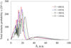 |
Fig. 1 Dependence of total inelastic transition probability on the impact parameter, often known as the partial cross section, for the initial state 111000 of the H2O + H2O system. Different colors correspond to different collision energies (temperatures) as labeled in the figure. |
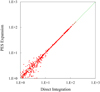 |
Fig. 2 Comparison of matrix elements computed by PES expansion vs. direct integration method for the 515422 → 524431 transition in the H2O + H2O system, near R = 6 and 8 Bohr. The unit of the matrix elements is cm−1. |
3 Results and discussion
Within the theoretical framework described above, we calculated all state-to-state transition cross sections  between the rotational states of the H2O + H2O system. The overall number of individual state-to-state transitions
  is huge, on the order of 3.5 million. In Fig. 3, we plot these data for T = 600 K as a function of total energy transfer ∆E in the H2O + H2O system (as a whole), without any averaging. Out of the 3.5 million transitions in total, about 2 million transitions have cross sections above 0.01 Å2.
Qualitatively, the dependence in Fig. 3 represents a rather typical double-exponential character of the collisional energy transfer (Ivanov & Babikov 2011; Ivanov & Schinke 2005). In the vicinity of the elastic peak (∆E ~ 0), the values of the cross sections drop quickly, but around |∆E| ~ 70 cm−1 ‚ this trend switches to a much slower decay. The excitation wing (∆E > 0) and quenching wing (∆E < 0) exhibit similar slopes. For each value of ∆E, the distribution of the cross section values is rather broad (at least one order of magnitude wide) which means that in addition to ∆E, other properties of the initial and final states affect the values of individual cross sections. Consequently, the accurate fitting of these data by a simple analytic function may be challenging, if it is possible at all. Figure A.1 shows these data near ∆E ~ 0 in detail. In the vicinity of the elastic peak, the majority of the cross sections are on the order of 100–200 Å2, although some of them are larger. For example, the highest cross section value of σ = 599 Å2 in Fig. 3 corresponds to the 000422 → 111413 transition.
From MQCT data for the individual state-to-state transitions (see Fig. 3), we computed thermally averaged cross sections  for 231 transitions in para- and 210 transitions in ortho-H2O, including excitation and quenching processes for each transition (882 TACS total). These are plotted in Fig. 4 against the value of the energy transfer in the target H2O molecule, ∆E1, at the temperature of T = 600 K. Overall, the dependence is similar to what we saw in Fig. 3. The excitation and quenching wings have similar slopes, and the majority of TACS within the wings fall in the range of
  . A compact group of large cross sections in the range
  corresponds to dipole-driven transitions, with the largest being
  for 000 → 111 process. Another group of very small TACS is seen below the quenching wing in Fig. 4. They correspond to the quenching of highly excited rotational states onto the ground-state 000. This group of transitions appears as outliers in Fig. 4 because for any j = 1 and higher, both para- and ortho-states are available, while for j = 0, there is only a para state. Therefore, this one para-state is more distant from (less connected to) the excited states than all other states available for transitions.
At this point, we would like to mention that the full quantum methods are expected to give state-to-state transition cross sections that automatically satisfy the principle of microscopic reversibility. In practice, this requires a good level of numerical convergence, which is often hard to achieve. This property is not built in automatically in the mixed quantum-classical method (Babikov & Semenov 2016; Semenov & Babikov 2013a). Therefore, the matrix of state-to-state transition cross sections computed by MQCT needs to be symmetrized (Boursier et al. 2020) before it can be used to model energy transfer kinetics. Microscopic reversibility is satisfied if for any two states j and j′, the following relation holds:
 (3)
(3)
In this formula, thermal weights w(T) and thermally averaged cross sections  correspond to the same temperature T, and it is assumed that the energy change of the transition n → n′ is much smaller than kT. In order to determine the degree to which the relation of Eq. (3) is violated, the values of state-to-state transition cross sections that are computed directly by MQCT (which we call the “direct” TACS) can be used to compute the values of cross sections for transitions in the reverse direction (which we call the “reverse” TACS) for the same temperature,
 (4)
(4)
A comparison of the direct and reverse TACS is presented in Fig. 5 at T = 600 K (Fig. A.2 gives a summary of these data for six different temperatures). These figures show that the principle of microscopic reversibility is approximately satisfied. The deviations remain small through several orders of magnitude of cross section values. Smaller cross sections tend to have larger relative deviations, and these are somewhat larger for lower temperatures (see the appendix).
In order to quantify these differences, we computed deviations of the reverse TACS from the direct TACS for each state-to-state transition and plotted them as percent of the cross section value. They are presented in Fig. 6 for T = 600 K (Fig. A3 gives a summary of these data for six different temperatures). Figure 6 shows that for larger cross sections,  , the deviations are ~ 10% or smaller. For smaller cross sections, the deviations are larger. For example, for the smallest cross section, on the order of
  ‚ the deviation is ~20%. For lower temperatures, the deviations show a similar trend, but are somewhat larger (see the appendix).
Two strategies can produce a symmetric TACS matrix that exactly satisfies the principle of microscopic reversibility. One method is to keep only a half of the computed cross sections (e.g., for quenching) and to replace the other half (for excitation) with the values computed in reverse using Eq. (4). Another approach is to use all computed cross sections to symmetrize the matrix by calculating the average of the left- and right-hand sides of Eq. (3) and by dividing it by the appropriate weight, namely
 (5)
(5)
 (6)
(6)
We followed the second method and found that the RMSD of TACS in the original dataset from the final symmetrized version are only 0.44, 0.53, 0.68, and 1.47 Å2 for T = 600, 450, 300, and 150 K, respectively, which indicates that the original MQCT dataset was already very close to symmetric. For example, if the differences between direct and reverse TACS discussed above were within 10% of each other (see Fig. 6), they would be within 5% of the final dataset of symmetrized TACS. This is consistent with RMSD on the order of 0.5 Å2 for cross sections that are ~10 Å2, on average.
Our database includes 443 quenching transitions (see above). The oldest database of Buffa et al. (2000) includes 173 quenching cross sections for H2O + H2O system, out of which 56 are included in our database. The more recent database of Boursier et al. (2020) includes 1299 quenching cross sections, out of which 246 cross sections can be found in our database. Therefore, a comparison of all three datasets is possible and is presented in Fig. 7 for T = 600 K. Additionally, Fig. A.4 shows a comparison for temperatures of T = 800 and 300 K. Figure 7 shows that our cross sections are close to the results of Boursier et al. (2020) for the transitions in their database with cross-section values on the order of  (i.e., not too high and not too low). These processes represent the main transition group in the system that are not driven by the dipole-dipole interaction. It should be noted that these transitions are entirely absent in the database of Buffa et al. (2000) simply because these authors did not include any interactions beyond the dipole-dipole.
For the group of smaller cross sections,  , our MQCT results are systematically larger than the results of Boursier et al. (2020), which were obtained using a semiclassical method. Figure 5 indeed shows that only a few MQCT TACS have values of
  , and no MQCT TACS has values of
  . This is in sharp contrast with the dataset of Boursier et al. (2020), which contains many transitions with small cross sections. We conclude that for transitions characterized by small TACS, the MQCT method gives larger cross sections than a semiclassical method. This observation can be explained by the fact that in MQCT calculations, all states are coupled by ladderlike transitions, and even if the direct coupling between a pair of states is small, the transition may still proceed through a dense manifold of the neighboring states. As a simplified example, we can consider a system of three consecutive states A, B, and C, among which only the immediate neighbors are coupled, and adopt a quantum time-dependent viewpoint, where the collision event occurs during some finite (nonzero) time interval. If at the initial moment in time the system is in state A, then, during the collision event, not only state B, but also state C will be excited with some probability because of the ladder-like process that starts populating C as soon as some population is transferred to state B. In the semiclassical method, in contrast, each state-to-state transition is described independently from others. This artificially makes some transitions too weak.
For the same reason, in the group of processes that is characterized by larger cross sections driven by the dipole-dipole interaction,  , our MQCT results are systematically smaller than those of either Boursier et al. (2020) or Buffa et al. (2000), obtained using semiclassical methods (see Fig. 7). Our explanation for this observation is that simultaneously with strong dipole-driven transitions that populate some states, MQCT calculations also include transitions that depopulate these states, transferring a part of population to their neighbors. In the semiclassical methods, these secondary processes are neglected, which artificially makes the dipole-driven transitions too strong. For these transitions, our MQCT TACS are somewhat closer to those of Buffa et al. (2000) than to those of Boursier et al. (2020). For the dipoledriven transitions, our results are 31% smaller on average than those of Buffa et al. (2000), and they are 44% smaller than those of Boursier et al. (2020). The corresponding RMSD are about 20 and 36 Å2, respectively. These numbers should be compared to the average values of dipole-driven transitions in three databases: 43, 62, and 78 Å2. The differences between Buffa et al. (2000) and Boursier et al. (2020) are likely due to different choices of interaction parameters because in all other aspects, the methods of Buffa et al. (2000) and Boursier et al. (2020) are very similar. The differences between MQCT and the two older databases come both from the PES representation (more accurate in our calculations) and from the description of molecule-molecule collision event (also more rigorous in MQCT).
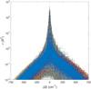 |
Fig. 3 Correlation between the values of individual state-to-state cross sections |

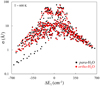 |
Fig. 4 Correlation between the values of thermally averaged state-to-state cross sections |

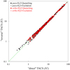 |
Fig. 5 Comparison of thermally averaged cross sections (TACS) |

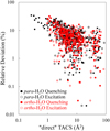 |
Fig. 6 Percent deviation of reverse TACS from direct TACS for various transitions in H2O at T = 600 K. |
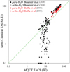 |
Fig. 7 Comparison of TACS computed by semiclassical methods and MQCT. The MQCT results are larger than the two semiclassical methods for low TACS values, and they are smaller for higher TACS values. |
4 Conclusions
In this paper, we described new calculations of cross sections for the individual rotational state-to-state transitions in H2O + H2O collisions, using the mixed quantum-classical theory approach implemented in MQCT code. A large basis set of rotational states was used in these calculations and permitted us to predict thermally averaged cross sections for 441 transitions in para-and ortho-H2O in a broad range of temperatures, from which we generated a new database of collisional rate coefficients for cometary and planetary applications. Although our database includes fewer transitions than the two older databases, this new set of data is expected to be more reliable because our MQCT theory is more rigorous (compared to the semiclassical method), both in terms of representation of the PES for H2O + H2O interaction and in terms of the description of H2O + H2O collision dynamics. The internal convergence of the MQCT calculations with respect to the input parameters (e.g., rotational basis set size and the truncation of the PES expansion) is estimated to be within few percent of the thermally averaged cross section values.
However, the MQCT approach itself is also an approximate method (e.g., compared to the full-quantum approach), and it therefore carries some intrinsic errors that can be estimated based on the deviation of MQCT cross sections for excitation and quenching processes from the principle of microscopic reversibility. This gives theoretical error bars that depend on temperature. At T = 600 K, the accuracy is estimated to be within 5% for cross sections larger than 10 Å2 and within 10% for smaller cross sections. For lower temperatures, the errors are larger. For example, at T = 200 K, the errors are within 5% for the largest cross sections (which are on the order of 100 Å2), but they increase to 40% for smallest cross sections (which are on the order of 1 Å2).
This level of accuracy is appropriate for an astrophysical modeling of radiative energy transfer using such codes as RADEX (Van der Tak et al. 2007) or LIME (Brinch & Hogerheijde 2010). Detailed information about these errorbars is available from Fig. A.3. The values of thermally averaged cross sections (TACS), symmetrized to satisfy the principle of microscopic reversibility, are available at six temperatures: T = 800, 600, 450, 300, 275, and 150 K. Since the dependence of each TACS on temperature is smooth, we also wrote a user-ready program that interpolates our data using a standard cubic-spline technique to give a continuous temperature function in the range from T = 150 to 800 K for all TACS. This program is available for download from CDS.
Although in the past, the MQCT method has been used to compute state-to-state transition cross sections for a variety of molecular processes, this paper reports the first application of the MQCT program for the generation of a database of rate coefficients that are suitable for astronomical and astrophysical applications. In the future, we will expand this approach to other molecules and quenchers, but may also try to improve several aspects of the work reported here. For example, here we computed thermal rate coefficients as  , where
  is the thermally averaged cross section. This simple expression is approximate. Namely, it assumes that the energy dependence of cross sections
  is weak. A more rigorous approach includes the prediction of the actual
  dependence in a broad range of energies, followed by averaging of
  over the Maxwell–Boltzmann distribution. This will be one direction of future work.
Another direction of future work could be to expand the range of temperatures covered here into the low-T region, because the kinetic temperature in a cometary coma can be much lower than 150 K. In principle, the program written to interpolate our rate coefficients (supplied with this paper) can also be used for extrapolation outside of the covered range, but this must be done with caution, since the general cubic spline does not guarantee a physically correct asymptotic behavior. A better approach would be to perform calculations at lower temperatures. We stopped at 150 K because we saw that our MQCT results started to deviate significantly from the principle of microscopic reversibility (see Figs. A.2 and A.3). While currently, MQCT is the only method implemented for the asymmetric top rotor + asymmetric top rotor system (to our best knowledge), it is known that it becomes less accurate at lower collision energies (temperatures). Some other approximate quantum methods, such as the recently developed statistical method (Faure et al. 2020), which is known to be sufficiently accurate at low collision energies, could provide an alternative tool. One interesting approach to explore in the future would be to blend the statistical method at low energies with the MQCT method at high energies to cover the entire energy range.
Acknowledgements
This research was supported by NASA Astrophysics Program, grant number NNX17AH16G. D.B. acknowledges the support of Way Klingler Research Fellowship. B.M. acknowledges the support of Denis J. O’Brien and Eisch Fellowships. We used resources of the National Energy Research Scientific Computing Center, which is supported by the Office of Science of the U.S. Department of Energy under Contract No. DE-AC02-5CH11231. This research also used HPC resources at Marquette funded in part by the National Science foundation award CNS-1828649. Marie-Lise Dubernet at the Observatory of Paris is gratefully acknowledged for her continuous support of these efforts. Martin Cordiner at NASA is acknowledged for stimulating discussions and his encouragement of this project.
Appendix A Additional figures
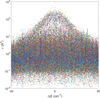 |
Fig. A.1 Same as Fig. 3 in the main text, but here the focus is on the range of small energy transfer, −50 ≤ ∆E ≤ 50 cm−1, to explore the behavior near the peak in more detail. |
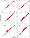 |
Fig. A.2 Same as Fig. 5 in the main text, but here the data for six different temperatures are collected: T = 800, 600, 450, 300, 225, and 150 K. |
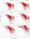 |
Fig. A.3 Same as Fig. 6 in the main text, but here the data for six different temperatures are collected: T = 800, 600, 450, 300, 275, and 150 K. |
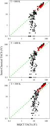 |
Fig. A.4 Same as Fig. 7 in the main text, but here the data for three different temperatures are collected: T = 800, 600, and 300 K. |
References
- Al-Edhari, A.J., Ceccarelli, C., Kahane, C., et al. 2017, A&A, 597, A40 [NASA ADS] [CrossRef] [EDP Sciences] [Google Scholar]
- Altwegg, K., Balsiger, H., Bar-Nun, A., et al. 2015, Science, 347, 1261952 [Google Scholar]
- Babikov, D., & Semenov, A. 2016, J. Phys. Chem. A, 120, 319 [NASA ADS] [CrossRef] [Google Scholar]
- Bannister, M.T., Bhandare, A., Dybczynski, P.A., et al. 2019, Nat. Astron., 3, 594 [NASA ADS] [CrossRef] [Google Scholar]
- Bockelée-Morvan, D., Hartogh, P., Crovisier, J., et al. 2010, A&A, 518, A149 [Google Scholar]
- Bockelée-Morvan, D., Calmonte, U., Charnley, S., et al. 2015, Space Sci. Rev., 197, 47 [Google Scholar]
- Bonev, B.P., Russo, N.D., DiSanti, M.A., et al. 2021, Planet. Sci. J., 2, 45 [NASA ADS] [CrossRef] [Google Scholar]
- Boursier, C., Mandal, B., Babikov, D., & Dubernet, M. 2020, MNRAS, 498, 5489 [NASA ADS] [CrossRef] [Google Scholar]
- Brinch, C., & Hogerheijde, M. 2010, A&A, 523, A25 [NASA ADS] [CrossRef] [EDP Sciences] [Google Scholar]
- Bruzzone, L., Plaut, J.J., Alberti, G., et al. 2013, in 2013 IEEE International Geoscience and Remote Sensing Symposium-IGARSS, IEEE, 3907 [CrossRef] [Google Scholar]
- Buffa, G., Tarrini, O., Scappini, F., & Cecchi-Pestellini, C. 2000, ApJS, 128, 597 [NASA ADS] [CrossRef] [Google Scholar]
- Caselli, P., Keto, E., Pagani, L., et al. 2010, A&A, 521, A29 [NASA ADS] [CrossRef] [EDP Sciences] [Google Scholar]
- Ceccarelli, C., Caselli, P., Bockelée-Morvan, D., et al. 2014, Protostars and Planets VI, eds. H. Beuther, R.S. Klessen, C.P. Dullemond, & T. Henning (Tucson: University of Arizona Press), 859 [Google Scholar]
- Cencek, W., Szalewicz, K., Leforestier, C., van Harrevelt, R., & van der Avoird, A. 2008, Phys. Chem. Chem. Phys., 10, 4716 [CrossRef] [Google Scholar]
- Chen, W., & Neufeld, D.A. 1995, ApJ, 453, L99 [NASA ADS] [CrossRef] [Google Scholar]
- Cochran, A.L., Levasseur-Regourd, A.-C., Cordiner, M., et al. 2015, Space Sci. Rev., 197, 9 [CrossRef] [Google Scholar]
- Codella, C., Ceccarelli, C., Cabrit, S., et al. 2016, A&A, 586, A3 [Google Scholar]
- Cordiner, M., Milam, S., Biver, N., et al. 2020, Nat. Astron., 4, 861 [NASA ADS] [CrossRef] [Google Scholar]
- Coutens, A., Vastel, C., Caux, E., et al. 2012, A&A, 539, A132 [NASA ADS] [CrossRef] [EDP Sciences] [Google Scholar]
- Dones, L., Brasser, R., Kaib, N., & Rickman, H. 2015, Space Sci. Rev., 197, 191 [NASA ADS] [CrossRef] [Google Scholar]
- Enya, K., Kobayashi, M., Kimura, J., et al. 2022, Adv. Space Res., 69, 2283 [NASA ADS] [CrossRef] [Google Scholar]
- Faure, A., & Josselin, E. 2008, A&A, 492, 257 [NASA ADS] [CrossRef] [EDP Sciences] [Google Scholar]
- Faure, A., Lique, F., & Remijan, A.J. 2018, J. Phys. Chem. Lett., 9, 3199 [NASA ADS] [CrossRef] [Google Scholar]
- Faure, A., Hily-Blant, P., Rist, C., et al. 2019, MNRAS, 487, 3392 [Google Scholar]
- Faure, A., Lique, F., & Loreau, J. 2020, MNRAS, 493, 776 [NASA ADS] [CrossRef] [Google Scholar]
- Fitzsimmons, A., Snodgrass, C., Rozitis, B., et al. 2018, Nat. Astron., 2, 133 [Google Scholar]
- Fitzsimmons, A., Hainaut, O., Meech, K.J., et al. 2019, ApJ, 885, L9 [NASA ADS] [CrossRef] [Google Scholar]
- Guzik, P., Drahus, M., Rusek, K., et al. 2020, Nat. Astron., 4, 53 [Google Scholar]
- Hama, T., Kouchi, A., & Watanabe, N. 2016, Science, 351, 65 [NASA ADS] [CrossRef] [Google Scholar]
- Hartogh, P., Lellouch, E., Moreno, R., et al. 2011, A&A, 532, A2 [CrossRef] [EDP Sciences] [Google Scholar]
- Henning, T., & Semenov, D. 2013, Chem. Rev., 113, 9016 [Google Scholar]
- Humphreys, E. 2007, Proc. Int. Astron. Union, 3, 471 [NASA ADS] [CrossRef] [Google Scholar]
- Ivanov, M.V. & Babikov, D. 2011, J. Chem. Phys., 134, 174308 [NASA ADS] [CrossRef] [Google Scholar]
- Ivanov, M.V., & Schinke, R. 2005, J. Chem. Phys., 122, 234318 [NASA ADS] [CrossRef] [Google Scholar]
- Jankowski, P., Murdachaew, G., Bukowski, R., et al. 2015, J. Phys. Chem. A, 119, 2940 [NASA ADS] [CrossRef] [Google Scholar]
- Jehin, E., Bockelée-Morvan, D., Dello Russo, N., et al. 2009, Earth, Moon, and Planets, 105, 343 [NASA ADS] [CrossRef] [Google Scholar]
- Jensen, S., Jørgensen, J., Kristensen, L., et al. 2019, A&A, 631, A25 [NASA ADS] [CrossRef] [EDP Sciences] [Google Scholar]
- Jensen, S., Jørgensen, J., Kristensen, L., et al. 2021, A&A, 650, A172 [NASA ADS] [CrossRef] [EDP Sciences] [Google Scholar]
- Jewitt, D., Luu, J., Rajagopal, J., et al. 2017, ApJ, 850, L36 [NASA ADS] [CrossRef] [Google Scholar]
- Jewitt, D., Hui, M.-T., Kim, Y., et al. 2020, ApJ, 888, L23 [NASA ADS] [CrossRef] [Google Scholar]
- Kaufman, M.J., & Neufeld, D.A. 1996, ApJ, 456, 611 [NASA ADS] [CrossRef] [Google Scholar]
- Khalifa, M.B., Quintas-Sánchez, E., Dawes, R., Hammami, K., & Wiesenfeld, L. 2020, Phys. Chem. Chem. Phys., 22, 17494 [NASA ADS] [CrossRef] [Google Scholar]
- Lis, D.C., Bergin, E.A., Schilke, P., & Van Dishoeck, E.F. 2013, J. Phys. Chem. A, 117, 9661 [NASA ADS] [CrossRef] [Google Scholar]
- Mandal, B., Semenov, A., & Babikov, D. 2018, J. Phys. Chem. A, 122, 6157 [NASA ADS] [CrossRef] [Google Scholar]
- Mandal, B., Semenov, A., & Babikov, D. 2020, J. Phys. Chem. A, 124, 9877 [NASA ADS] [CrossRef] [Google Scholar]
- Mandal, B., Joy, C., Semenov, A., & Babikov, D. 2022, ACS Earth Space Chem., 6, 521 [NASA ADS] [CrossRef] [Google Scholar]
- Mandal, B., Joy, C., Bostan, D., Eng, A., & Babikov, D. 2023, J. Phys. Chem. Lett., 14, 817 [CrossRef] [Google Scholar]
- Mas, E.M., Szalewicz, K., Bukowski, R., & Jeziorski, B. 1997, J. Chem. Phys., 107, 4207 [NASA ADS] [CrossRef] [Google Scholar]
- Meech, K.J., Weryk, R., Micheli, M., et al. 2017, Nature, 552, 378 [NASA ADS] [CrossRef] [Google Scholar]
- Micheli, M., Farnocchia, D., Meech, K.J., et al. 2018, Nature, 559, 223 [NASA ADS] [CrossRef] [Google Scholar]
- Opitom, C., Fitzsimmons, A., Jehin, E., et al. 2019, A&A, 631, A8 [NASA ADS] [CrossRef] [EDP Sciences] [Google Scholar]
- Putaud, T., Michaut, X., Le Petit, F., Roueff, E., & Lis, D. 2019, A&A, 632, A8 [NASA ADS] [CrossRef] [EDP Sciences] [Google Scholar]
- Roth, N.X., Bonev, B.P., DiSanti, M.A., et al. 2021, Planet. Sci. J., 2, 54 [NASA ADS] [CrossRef] [Google Scholar]
- Roueff, E., & Lique, F. 2013, Chem. Rev., 113, 8906 [Google Scholar]
- Sakai, N., Oya, Y., Sakai, T., et al. 2014, ApJ, 791, L38 [Google Scholar]
- Schroeder, I.R., Altwegg, K., Balsiger, H., et al. 2019, A&A, 630, A29 [NASA ADS] [CrossRef] [EDP Sciences] [Google Scholar]
- Semenov, A., & Babikov, D. 2013a, J. Chem. Phys., 138, 164110 [NASA ADS] [CrossRef] [Google Scholar]
- Semenov, A., & Babikov, D. 2013b, J. Chem. Phys., 139, 174108 [NASA ADS] [CrossRef] [Google Scholar]
- Semenov, A., & Babikov, D. 2014a, J. Phys. Chem. Lett., 5, 275 [CrossRef] [Google Scholar]
- Semenov, A., & Babikov, D. 2014b, J. Chem. Phys., 140, 044306 [NASA ADS] [CrossRef] [Google Scholar]
- Semenov, A., & Babikov, D. 2015, J. Phys. Chem. Lett., 6, 1854 [CrossRef] [Google Scholar]
- Semenov, A., & Babikov, D. 2017, J. Phys. Chem. A, 121, 4855 [NASA ADS] [CrossRef] [Google Scholar]
- Semenov, A., Mandal, B., & Babikov, D. 2020, Comput. Phys. Commun., 252, 107155 [NASA ADS] [CrossRef] [Google Scholar]
- Taquet, V., Peters, P., Kahane, C., et al. 2013, A&A, 550, A127 [NASA ADS] [CrossRef] [EDP Sciences] [Google Scholar]
- Tielens, A.G. 2005, The Physics and Chemistry of the Interstellar Medium (Cambridge University Press) [CrossRef] [Google Scholar]
- Tielens, A.G., & Allamandola, L.J. 1987, in Interstellar Processes (Springer), 397 [NASA ADS] [CrossRef] [Google Scholar]
- Van der Tak, F., Black, J.H., Schöier, F., Jansen, D., & van Dishoeck, E.F. 2007, A&A, 468, 627 [NASA ADS] [CrossRef] [EDP Sciences] [Google Scholar]
- van Dishoeck, E.F., Kristensen, L., Benz, A., et al. 2011, PASP, 123, 138 [NASA ADS] [CrossRef] [Google Scholar]
- van Dishoeck, E.F., Kristensen, L.E., Mottram, J.C., et al. 2021, A&A, 648, A24 [NASA ADS] [CrossRef] [EDP Sciences] [Google Scholar]
- Vorburger, A., Fatemi, S., Galli, A., et al. 2022, Icarus, 375, 114810 [NASA ADS] [CrossRef] [Google Scholar]
- Wirström, E., Bjerkeli, P., Rezac, L., Brinch, C., & Hartogh, P. 2020, A&A, 637, A90 [NASA ADS] [CrossRef] [EDP Sciences] [Google Scholar]
- Yang, B., Li, A., Cordiner, M.A., et al. 2021, Nat. Astron., 5, 586 [CrossRef] [Google Scholar]
All Figures
|
Fig. 1 Dependence of total inelastic transition probability on the impact parameter, often known as the partial cross section, for the initial state 111000 of the H2O + H2O system. Different colors correspond to different collision energies (temperatures) as labeled in the figure. |
| In the text | |
|
Fig. 2 Comparison of matrix elements computed by PES expansion vs. direct integration method for the 515422 → 524431 transition in the H2O + H2O system, near R = 6 and 8 Bohr. The unit of the matrix elements is cm−1. |
| In the text | |
|
Fig. 3 Correlation between the values of individual state-to-state cross sections |
| In the text | |
|
Fig. 4 Correlation between the values of thermally averaged state-to-state cross sections |
| In the text | |
|
Fig. 5 Comparison of thermally averaged cross sections (TACS) |
| In the text | |
|
Fig. 6 Percent deviation of reverse TACS from direct TACS for various transitions in H2O at T = 600 K. |
| In the text | |
|
Fig. 7 Comparison of TACS computed by semiclassical methods and MQCT. The MQCT results are larger than the two semiclassical methods for low TACS values, and they are smaller for higher TACS values. |
| In the text | |
|
Fig. A.1 Same as Fig. 3 in the main text, but here the focus is on the range of small energy transfer, −50 ≤ ∆E ≤ 50 cm−1, to explore the behavior near the peak in more detail. |
| In the text | |
|
Fig. A.2 Same as Fig. 5 in the main text, but here the data for six different temperatures are collected: T = 800, 600, 450, 300, 225, and 150 K. |
| In the text | |
|
Fig. A.3 Same as Fig. 6 in the main text, but here the data for six different temperatures are collected: T = 800, 600, 450, 300, 275, and 150 K. |
| In the text | |
|
Fig. A.4 Same as Fig. 7 in the main text, but here the data for three different temperatures are collected: T = 800, 600, and 300 K. |
| In the text | |
Current usage metrics show cumulative count of Article Views (full-text article views including HTML views, PDF and ePub downloads, according to the available data) and Abstracts Views on Vision4Press platform.
Data correspond to usage on the plateform after 2015. The current usage metrics is available 48-96 hours after online publication and is updated daily on week days.
Initial download of the metrics may take a while.