| Issue |
A&A
Volume 671, March 2023
|
|
|---|---|---|
| Article Number | A27 | |
| Number of page(s) | 9 | |
| Section | Stellar atmospheres | |
| DOI | https://doi.org/10.1051/0004-6361/202245384 | |
| Published online | 02 March 2023 | |
Infrared He I 10830 Å, ultra-violet Ca II, and Mg II chromosphere emissions in the spectra of classical Cepheid X Cyg
1
Astronomical Observatory, Odessa National University of the Ministry of Education and Science of Ukraine,
Shevchenko Park,
65014
Odessa, Ukraine
e-mail: This email address is being protected from spambots. You need JavaScript enabled to view it.
2
Institut für Astronomie und Astrophysik, Kepler Center for Astro and Particle Physics, Universität Tübingen,
Sand 1,
72076
Tübingen, Germany
3
GEPI, Observatoire de Paris, Université PSL, CNRS,
5 Place Jules Janssen,
92190
Meudon, France
4
Physics of stars department, Crimean Astrophysical Observatory,
Nauchny
298409, Crimea
Received:
6
November
2022
Accepted:
21
December
2022
Abstract
Aims. In a previous publication, we reported the first detection of emission in the infrared (IR) triplet at 10 830 Å in the spectra of the classical Cepheid X Cyg. Emission is detectable at phases from approximately 0.25 to 0.90. We present and discuss further information on the chromosphere activity of this star, namely International Ultraviolet Explorer (IUE) archive data concerning the emission in the h and k Mg II doublet, and near-ultraviolet (NUV) spectra in the vicinity of the H and K Ca II doublet. We also present rough estimates of the chromosphere conditions and semi-empirical modelling of the observed emissions in He I triplet.
Methods. A study of the emissions in UV lines of Ca II and Mg II, and IR lines of He I suggests that the emissions observed at certain phases can be explained within the framework of the Gillet's phenomenological model of shock waves in pulsating atmospheres, which was developed from a study of the Hα behaviour in X Cyg spectra. We used the non-local thermodynamic equilibrium (NLTE) approximation and a simple model of this star's chromosphere for the analysis of the chromosphere indicator profiles.
Results. We show that under certain assumptions about the properties of the chromosphere, it is possible to describe the presence or absence of emission in the IR lines of He I and Ca II, and UV lines of Ca II and Mg II.
Key words: stars: atmospheres / stars: chromospheres / stars: variables: Cepheids
© The Authors 2023
 Open Access article, published by EDP Sciences, under the terms of the Creative Commons Attribution License (https://creativecommons.org/licenses/by/4.0), which permits unrestricted use, distribution, and reproduction in any medium, provided the original work is properly cited.
This article is published in open access under the Subscribe to Open model. This email address is being protected from spambots. You need JavaScript enabled to view it. to support open access publication.
1 Introduction
The large-scale dynamical phenomena in the gas of the stellar atmosphere can lead to additional heating of the upper layers of the atmosphere to the values significantly exceeding the effective temperature of the star. This can lead to the formation of a kind of stellar chromosphere, or even a corona. This phenomenon can be found in pulsating variable stars. The main triggering mechanism forcing the surface layers of a star to participate in the pulsation process is related to the atmosphere gas opacity, and its behaviour under changing thermodynamic conditions. When the atmosphere gas is compressed (the star contracts due to the gravitational attraction of previously expanded envelopes), energy is distributed through various channels. In particular, it goes to additional ionisation of partially ionised species, such as He II. The shell of the partially ionised helium acts as a destabilising zone in many types of pulsating stars. During the contraction, the gas density in this zone increases, while the local temperature shows almost no increase (energy loss through further ionisation), and so the maxima of the density and temperature do not coincide in time. When a gas (namely, its most abundant components helium and hydrogen) becomes fully ionised in this zone, it behaves like an ideal gas, and therefore the kinetic energy of the particles of such a gas increases. This means that the temperature of the gas increases and its opacity decreases. The stellar atmosphere layers begin to expand. An interaction between the different layers forms an acoustic wave at this time. Propagating upwards in the atmosphere through a gas of decreasing density, this wave must accelerate significantly (however, see Gillet & Fokin 2014 and discussion below). At a certain velocity, the wave becomes a shock wave and through its dissipation effectively heats the gas. The heated zone behind the shock wave front and the pre-heating zone in front of the viscous jump can provide a source of high-energy radiation. This mechanism may manifest itself as energy emission in typical chromospheric lines, such as UV H and K Ca II, h and k Mg II, the IR Ca II triplet, He I 10 830 Å triplet lines, and others.
Pioneering works on the chromospheric activity of radially pulsating variable stars, namely the Cepheids, focused on ground-based observations of the NUV lines of the Ca II H and K doublet. Relevant papers have been published, for example, by Adams & Joy (1939), Van Hoof (1948), and Joy & Wilson (1949). Kraft (1957) lists all the papers on the UV Ca II emission published before 1957. All of the studied Cepheids have pulsation periods of more than 5 days. Later, Hollars (1974) described the K Ca II emission on the rising part of the light curve of a short-period (≈3.7 days) classical Cepheid RT Aur (emission was detected at phase close to 0.9).
A new era of studying the chromospheric emission in pulsating stars began with the IUE space mission. Detection of chromospheric UV h and k Mg II emission in the Cepheid spectra has been reported, for example, by Parsons (1980). The author reported results of a low- and high-resolution IUE spectral analysis of classical Cepheids, typically at phases 0.7–1.0. A very interesting result was obtained for two stars: δ Cep and β Dor. While the latter star shows Mg II and O I emissions at all observed phases, the former does not (on the observed phases). Earlier, Schmidt & Weiler (1979) in their study of h and k Mg II emission in Cepheid β Dor (Copernicus satellite data) indicated that emission is stronger near minimum light and weaker near maximum light.
Schmidt & Parsons (1982a,b) described the results of the IUE program designed to search for chromospheric emissions in a limited sample of classical Cepheids (δ Cep, β Dor, η Aql, ζ Gem, l Car). Far-ultraviolet (FUV) line emissions (C IV, O I, Si II) in the wavelength range 1300–1900 Å were detected in three stars, as well as their variation with pulsation cycle. For instance, the emission in the line O II 1305 Å reaches a maximum at a phase of about 0.8–0.9 for β Dor; the same emission is seen at almost the same level throughout the entire pulsation cycle for ζ Gem; and its maximum level is observed at phases 0.0–0.1 for l Car. The fact that the emission behaviour differs from one star to another was emphasised by these authors.
Later, Schmidt & Parsons (1984a) reported results from their study of high-resolution IUE spectra in the vicinity of h and k Mg II lines in the spectra of the same five classical Cepheids. Emission was detected, but according to the authors, the average emission flux is lower than that of non-variable supergiants of the same spectral classes. In the phases of the strongest emission, the emission flux is comparable to that which is characteristic of non-variable supergiants of similar temperature. Table 4 from this latter work shows that the phases of emission growth in the Cepheids are distributed between 0.5 and 1.0.
Schmidt & Parsons (1984b) again undertook a search for lines in the UV region that could indicate a transition zone in Cepheids. In this latter study, the authors succeeded in detecting emission in the O I 1305 Å line for δ Cep, but it was significantly weaker than in the other Cepheids studied (β Dor and ζ Gem).
Engle et al. (2014) conducted a thorough study of δ Cep in the X-ray range (see discussion below) and in the FUV band using the HST – COS equipment. In particular, in UV band, these authors observed many important lines, and investigated the variability of the following lines in detail: O I 1358 Å, Si IV 1393/1403 Å, and N V 1239/1243 Å. Integrated fluxes in these lines show a peak value at a phase close to 0.0.
The UV h and k Mg II emissions have also been studied in other types of pulsating variable stars. Parthasarathy & Parsons (1984) presented the results of observations of two radially pulsating W Vir-type stars, AL Vir (P = 10.3 days) and W Vir (P = 17.3 days), noting that the low-dispersion UV spectra show a large range of h and k Mg II emission behaviour. We note that Kovtyukh et al. (2011) performed a multi-phase spectroscopic study of W Vir in order to trace the emission behaviour in the visual range of the spectrum. Various lines were used (Na I, Fe I, Fe II, Ba II, as well as hydrogen and helium lines). The authors concluded that the interaction of the main shock wave with the infalling envelope layers could explain the observed peculiarities of the spectral line variability.
Bonnell & Bell (1985) examined the IUE spectra of the radially pulsating RR Lyr-type stars: RR Lyr and X Ari. The high-and low-resolution spectra with good phase coverage showed no emission in the h and k Mg II lines. Ultraviolet chromospheric emission has also been detected from low-amplitude variable stars of δ Sct type. For example, Fracassini & Pasinetti (1982), Fracassini et al. (1983, 1991) and Teays et al. (1989) reported confident detections of h and k Mg II emissions in ρ Pup, β Cas, and τ Cyg. Emission was also suspected in some other stars of this type.
Pioneering works on observations and interpretation of the IR He I 10 830 Å triplet in Cepheid spectra were undertaken by Zirin (1975), η Aql, Sasselov & Lester (1994a), seven classical Cepheids with pulsation periods from 4 to 27 days (full-phase coverage was available for three of them), Sasselov & Lester (1994b,c). This IR triplet is a well-known chromosphere indicator because the corresponding radiative transition to a lower atomic level is forbidden, and it has an excitation potential of about 20 eV. A relatively detailed consideration of this triplet in the spectra of non-variable stars as well as a NLTE analysis can be found in O'Brien & Lambert (1986).
Sasselov & Lester (1994a) detected a helium line in six of the seven program stars. It is very interesting to note that the authors indicate that the helium triplet in ζ Gem is observed in both absorption and emission within the pulsation cycle. These authors pointed out that the helium triplet absorption in some stars is systematically blueshifted.
Sasselov & Lester (1994b) reported the first NLTE modelling of the helium triplet profile in the Cepheid spectra, and came to the conclusion that the chromospheres of the Cepheids are heated due to the dissipation of acoustic waves, which in turn is attributable to the pulsation dynamics. At the same time, the authors reject the existence of the hot coronae around Cepheid stars.
Very recently, Hocdé et al. (2020), see also references therein, considered the possibility that pulsation activity and periodic shocks in Cepheid atmospheres may be the source of ionised gas in the upper shells, and that these latter may have all the properties of a chromosphere. The authors studied the IR emission in classical Cepheids and concluded that variations occur in Hα and IR Ca II triplet for more than 20 Cepheids. For the shorter-period Cepheids of their sample, the authors note a weak blueshifted emission (inverse P Cyg profile) at phases between 0.6 and 0.9.
With the advent of new space missions, it has become possible to study radiation from pulsating variables in the X-ray region. Engle et al. (2014) observed five classical Cepheids with XMM-Newton and Chandra: SU Cas, Polaris, δ Cep, β Dor, and l Car. (Earlier, Evans et al. 2010 discussed the Chandra data for Polaris.) Engle et al. (2014) were only able to estimate the upper limit of the X-ray luminosity for the two program Cepheids with the shortest and longest periods, namely SU Cas and l Car. At the same time, X-ray activity was detected for δ Cep and β Dor. The flux reaches a maximum at a phase of about 0.5. Here we should also mention that probably the first attempt to detect X-ray emission from Cepheids was made by Böhm-Vitense & Parsons (1983). The authors observed δ Cep, β Dor, and ζ Gem with the Einstein Observatory facilities. X-ray emission was only suspected for ζ Gem at a pulsation phase of 0.26. Engle & Guinan (2012) reported HST - COS observations of Polaris, δ Cep, and β Dor. Their observations showed that these stars are indeed variable X-ray sources.
Engle et al. (2017) presented the results of XMM-Newton and Chandra observations of the classical Cepheid δ Cep. This pulsating star appeared to be a rather weak source of soft X-rays. Ultraviolet emissions attain their peak intensity at pulsation phases of approximately 0.6–0.9 (Engle et al. 2014), while Engle et al. (2017) found a peak in X-ray intensity at phase 0.45, for which they have no explanation. Despite the weak emission, these latter authors propose that δ Cep be considered the prototype of a new class of X-ray variable stars.
Evans et al. (2021) reviewed the results of the X-ray emission discovery in δ Cep and β Dor classical Cepheids and presented XMM-Newton observations of another bright classical Cepheid, η Aql, at a stage close to its maximum radius (when X-ray emission is observed in other Cepheids). The authors observed no X-ray radiation from this source. This seems strange, because η Aql and δ Cep (X-ray radiation was registered) have similar pulsation periods and spectral types.
It is also interesting to note that Oskinova et al. (2014) reported pulsation-phased X-ray emission from Alfirk (β Cep), which is a prototype β Cep-type star. It is believed that these hot stars with masses 10–15 M⊙ have shock waves in their envelopes, which are the results of the powerful pulsation motions.
From the above consideration, one can see that the appearance of chromosphere or corona emissions, activity maxima, and the duration of emission can differ from one star to another. More statistical data are needed to find the key factors responsible for the formation and activity of hot plasma envelopes of pulsating stars.
Of course, there is always some danger of mistakenly identifying the source of hard radiation as the Cepheid rather than its unresolved main sequence companion of late spectral type (if it exists). However, Engle et al. (2014) claim that hot plasma (with temperature up to 105 K) does exist in Cepheid atmospheres.
Having introduced the observational evidence pointing to chromosphere or corona activity in pulsating variable stars of several types, let us turn to our program star X Cyg. The first mention of chromospheric emission in our program star was made by Van Hoof (194), who found that the emission in the UV calcium lines is blueshifted in the spectrum and is strong between phases 0.9 and 1.0.
Later, Kraft (1957) studied the emission in the K Ca II line in more detail. Emission was observed between phases approximately from about 0.75 and 0.95 with an intensity peak near phase 0.9. After a decrease in emission intensity from peak towards the maximum light, a very strong increase in emission appears just after the maximum light, and then, at phase 0.05, the intensity drops to the peak value, which is observed before the maximum light. The emission near the maximum light is undetectable. It should be noted that the spectra fragments were not presented in this latter paper.
Wallerstein et al. (2019) conducted a study of the IR Ca II triplet in the X Cyg spectrum. In their Fig. 12, the authors present a detailed phase-resolved triplet profile variation. At most phases, the triplet lines are symmetric, while near the maximum light they become asymmetric and experience splitting. The Balmer Hα line shows similar behaviour. It is very important to note that the authors did not notice very weak emission in this triplet at phases 0.70, 0.71, and 0.77. These emissions are blueshifted (at about −60 km s−1; inverse P Cyg profile). These mentioned phases can be attributed to the secondary bump on the light curve. Relative to the γ-velocity, this emission layer is approaching with a velocity of approximately −20 km s−1. The above phases of the presence of the IR Ca II triplet emission coincide with the claimed phase visibility range of IR Ca II emission (0.6–0.9) in several Cepheids reported by Hocdé et al. (2020).
Detection of emission in the IR He I 10 830 Å triplet in the X Cyg spectrum was first reported in our previous paper (Kovtyukh et al. 2022; see Fig. 1 of that paper). In the present paper, we look in more detail at the characteristics of this emission, as well as the emissions in several other chromospheric indicators.
The shock waves generated by the radial pulsations of classical Cepheids and pulsation-dependent behaviour of the Hα emission associated with them have been the subject of theoretical works (see e.g. Fokin 1991, Gillet 2014). These authors did not consider the chromosphere emission in the chromosphere indicators, such as H and K Ca II, h and k Mg II, and some others.
Garbuzov & Andrievsky (1986), Andrievsky et al. (1987) and Andrievsky & Garbuzov (1991, 1992) proposed a mechanism that could explain the occurrence and variability of chromosphere emission in the Mg II h and k lines in the spectra of pulsating stars of the δ Sct type. According to the numerical model, the emission is due to the radiation of gas heated by a shock wave propagating in the outer layers of the stellar atmosphere at pulsation phases near maximum light. The flux variability in the Mg II h and k lines is due to the motion of the shock wave in the inhomogeneous medium with decreasing density. The authors succeeded in quantitatively reproducing the result of the IUE observations of the h and k emission flux in the spectrum of the δ Sct-type star ρ Pup (Fracassini & Pasinetti 1982).
Perhaps, the first analytical attempt to evaluate the capacity of radially pulsating RR Lyr-type stars to emit X-rays was made by Beigman & Stepanov (1981). These authors considered a strong shock wave arising during pulsation, the heating of proton gas at the viscous jump, and the subsequent energy redistribution between protons and electrons. The authors succeeded in showing that the post-shock region can be a source of energy emission from 1030 to 1032 erg s−1 in the soft-X-ray range of 80–200 Å.
A more detailed numerical consideration of soft X-ray emission from high-amplitude RR Lyrae pulsators was performed by Andrievsky & Matveev (1991). These authors took into account the energy distribution between a-particles, protons, and electrons. More precisely, the temperature variations of the different plasma components were determined by solving system kinetic equations describing the energy exchange between particles behind the shock front. It should be noted that the initial temperature at the viscous jump is significantly higher for helium ions than for protons. The authors showed that RR Lyr stars can be a source of soft-X-ray radiation (energies 0.1–0.2 keV).
A very detailed numerical consideration of the steady radiative shock waves propagating in the hydrogen stellar atmosphere gas was performed by Fadeyev & Gillet (1998). These authors constructed a shock-wave model that is based on a simultaneous self-consistent solution of the equations of fluid dynamics, radiative transfer, and population of energy levels of hydrogen atoms. Although the authors used 60 km s−1 as a maximum value of the shock-wave velocity, they obtained an electron temperature in the aftershock region on the order of several tens of thousands of Kelvin. Even higher values (about 105 K) were obtained in Fadeyev et al. (2002) for the slightly higher shock wave velocity.
Moschou et al. (2020) conducted a very detailed study of pulsation-driven shocks in Cepheids and considered the possibility that these shocks modulate the soft-X-ray emission flux. These authors succeeded in reproducing X-ray emission dominated by the shock-wave mechanism (the emission is present at phases 0.2–0.6). In general, we see that there is growing evidence that pulsating variable stars may possess chromosphere- or even corona-like envelopes, which are supplied with energy from their pulsation activity.
The present paper is organised as follows. In Sect. 2, we provide information on the available observations of our program star (in the visual range, in FUV, and in the IR region), which were used in the present consideration. The assumptions that we make regarding the chromosphere formation in this star are the subject of Sect. 3. In Sect. 4, we present our NLTE consideration of emission in the helium 10 830 Å triplet.
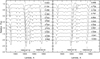 |
Fig. 1 Emission in the IR triplet in the spectra of X Cyg. Vertical dashed lines indicate phases with emission. Hereinafter, the phases are calculated according to Hintz et al. (2021). |
2 Observational resources
X Cyg is a classical Cepheid. Its pulsation period is 16.385692 days, its spectral type F7 Ib–G8 Ib, and the visual magnitude variation is in the range 5.85–6.91 (Szabados 1991). Here, we reproduce the figure from the paper of Kovtyukh et al. (2022), which shows spectrum changes in the vicinity of the He I triplet with some additions; spectra at additional phases were added (Fig. 1).
Spectra containing H and K Ca II lines were secured at the HARPS-N simultaneously with IR spectra (at the same phases). The resolving power of those spectra is 100 000. Figure 2 demonstrates the behaviour of the H and K Ca II lines in the spectra of the program star.
We also looked at the data from the archive of the IUE (ASCII table of large-aperture low-dispersion fluxes and wavelengths). X Cyg was observed about 20 times in the framework of the original observing program OD70Z (N.R. Evans). The results are summarised graphically in Fig. 3.
3 X Cyg chromosphere formation
Gillet (2014) performed a detailed consideration of the behaviour of the Hα line during the pulsation cycle in the X Cyg spectrum. The observed changes in the profile of this line with pulsation phase allowed him to create a phenomenological model of the shock-wave propagation in the envelope of this star, which is also applicable to other long-period Cepheids. Blueshifted emission is not observed in the Hα profile. Blueshifted absorption and redshifted emission (P Cyg profile) are present at phases from about 0.0 to 0.6. At phase 0.6, the Hα profile becomes absorptional and symmetric. Later, the line is split, with a redshifted absorptional component of growing intensity. Based on this evolution of the Hα profile over time, Gillet (2014) argued that there are two shock waves propagating in the X Cyg envelope at pulsation phases 0.0–0.3. One of them (the main shock generated by the current expansion) has not yet detached from the photosphere, while the second one (detached from the photosphere much earlier) is the shock wave that was generated during the previous pulsation cycle. At the next stage (phases from 0.3 to 0.6), the second shock wave disappears, while the main shock continues to develop and moves far from the photosphere boundary. Finally, at the phases before light maximum (0.6–0.9), a new shock wave emerges, which is caused by the falling layers of the atmosphere. Of course, such a picture is rather formal, but it seems capable of describing the behaviour of the Balmer Hα line. It should also be noted that the transition between the blueshifted emission (not actually seen in the X Cyg spectra) and blueshifted absorption probably occurs between phases 0.9 and 1.0. The author also argues that the study of the Hα profile indicates a relatively fast deceleration of the shock wave after its appearance in the upper atmosphere. The reason for this may be the effective radiative losses of the shock front in this zone. It should also be mentioned that a comprehensive analysis of the Hα line behaviour in several classic Cepheids was also performed earlier by Nardetto et al. (2008) using the very high-resolution spectra.
Previously, Gillet & Fokin (2014) analysed the behaviour of the Hα profile in another type of radial pulsator, the RR Lyrtype stars. Three emission features were explained by means of a hydrodynamic simulation. According to this latter, the first (blueshifted) strongest emission in Hα appears just before the maximum light (reversed Ρ Cyg profile; note again that such emission is not seen in the spectra of X Cyg). At this time, the shock wave has just detached from the photosphere. Then, a second, rather faint emission appears, which is redshifted along with blueshifted absorption (P Cyg profile; around phase 0.3). Much earlier, Hill (1972) in his theoretical consideration of the RR Lyrtype pulsations showed that two shock waves are formed in each period. Fokin (1992) came to the same conclusion.
Emission in the Η and Κ lines of Ca II in the X Cyg spectrum can be noted in the phase range from about 0.8 to 1.0 (see Fig. 2). Figure 3 shows the behaviour of the h and k Mg II lines in the X Cyg spectrum. We note that the spectra with close phases have been combined in order to reduce noise. Although the spectra are of low resolution, some emission-like features can be noted at phases from approximately 0.0 to 0.6. Another appearance of an emission-like structure at the phase around 0.8 is unclear, because immediately after that, at the phase around 0.9, no emission can be seen. It is interesting to note that UV Ca II emission first appears at close phase. Obviously, high-resolution UV data would be desirable to make the picture clearer. However, the real situation with the UV Mg II emission behaviour may actually be more complicated. As mentioned above, Fig. 3 shows that the emission was present at phase 0.55, it disappeared at phase 0.66 (pre-minimum radius), and reappeared again at phase 0.79. Perhaps to some extent this is similar to the behaviour of UV Ca II lines, where the emission disappears near the maximum light and suddenly is excited at the phase just after maximum light; see Sect. 1 and Kraft (1957).
The phase binding for the emissions in the UV Ca II (Fig. 2), Mg II (Fig. 3), and IR He I (Fig. 1) lines suggests the following: the H and Κ Ca II emissions are generated by the main shock wave not very far from the photosphere. This is also true for the emission observed in the h and k Mg II at phases near to the maximum light, h and k Mg II emissions observed in later phases should be excited higher up in the Cepheid envelope by the shock wave from the previous pulsation cycle. It is possible that, instead of a single main shock, two waves are generated before and near the maximum light. One is generated by the contracting atmosphere just before the minimum radius (phases around 0.8–0.9), and the second occurs just after the minimum radius, when the atmosphere begins to expand. Finally, the emission in He I lines also appears when the shock front(s) reaches the uppermost layers of the Cepheid envelope. This latter is probably generated in the infalling envelope layers and persists for a fairly long time interval, about 60% of the pulsation period. The formally estimated deceleration is very small: ΔV/Δt ≈ 5 km s−1/10 days ≈1 cm s−2 (see Fig. 2 in Kovtyukh et al. 2022 for explanation). A high-temperature zone, where He II lines emit energy, is heated by the shock waves travelling from the inner layers, and this zone may exist in the diluted medium for a long time. We note that the timing of the He I emissions is not directly connected to the photospheric phases presented in Fig. 4. The above reasoning is summarised in this latter figure schematically, including variation of the effective temperature to provide a visual reference to the phases in which emissions are observed.
To quantify the term 'uppermost layers' used above, we turned to the paper of Hocdé et al. (2021). The authors analysed mid-infrared (MIR) emission from the circumstellar envelope of the long-period Cepheid l Car, and concluded that a shell of ionised gas located at about 1.8 R* may be responsible for the observed feature. The radius of this star can be estimated from the period-radius relation of Gieren et al. (1999) for a pulsation period of 35.5 days: 160 R⊙. A shock front moving at a typical velocity of about 100 km s−1 from the photosphere will reach this layer in about 10 days. In the cases of X Cyg this time will clearly be shorter. Therefore, the IR helium emission can appear as early as a few days after the main shock wave detaches from the photosphere just before the maximum light. We would also like to note that Hocdé et al. (2020) find the chromosphere size in Cepheids to be about 50% of the stellar radius, that is of about 1012−1013 cm.
As the considered lines of Ca II and Mg II have different characteristics and the atoms and ions of these elements have different ionisation potentials as well (6.1 eV and 11.9 eV, 7.6 and 15.0 eV, respectively), the different behaviour of their emissions is to be expected. As stated by Schmidt & Weiler (1979) in their study of h and k Mg II emission in Cepheid β Dor, when the Mg II emission is most enhanced near minimum light, there is no Ca II emission (observations of Gratton 1953). On the other hand, near maximum light, Ca II emission is observed but the Mg II emission is less enhanced. The authors also conclude that Ca II emission is excited at the lower levels in the chromosphere, while Mg II originates in higher levels.
Cepheids are also known to show a different behaviour of Η and Κ Ca II and h and k Mg II emissions compared to the non-variable supergiants of similar spectral classes (see Sect. 1), and the emission properties and phase range of the emission presence are quite different for Cepheids with different pulsation periods (see e.g. Schmidt & Parsons 1984a, their Table 4 for five Cepheids with pulsation periods from 5 to 35 days). It should be noted that Böhm-Vitense & Dettmann (1980) investigated chromosphere (and transition-layer) emissions in non-variable stars with the help of IUE and found that late F and G supergiants with emissions are located only on the red side of the Cepheid instability strip on the HR diagram.
As mentioned above, Andrievsky & Matveev (1991) estimated the electron temperature behind the shock front by taking the shock wave velocity in the upper layers of the pulsating envelope of about 100 km s−1 (RR Lyr type stars). Shock waves of similar amplitudes have not been ruled out in the upper layers of the classical Cepheid envelopes (with typical radial-velocity amplitudes of about a few tens of km s−1 at the photosphere level; see e.g. Kiss 1998). Similar velocity values have also been predicted in the upper envelope layers of the Cepheid stars by Moschou et al. (2020); see their Fig. 3. Even assuming a typical velocity value of 100 km s−1, for the most abundant massive particles (protons and α-particles), we get a temperature at the viscous jump of the shock (more precisely, just behind the shock front)  , which is in the range of about 225 000 to 900 000 Κ (mp – mass of the particle, D – shock velocity, k – Boltzmann constant). For higher velocities, namely around 200 km s−1, these temperatures will significantly exceed these values (however, as noted above, Gillet 2014, after analysing Hα profile variation, concluded that the shock velocity decreases in the upper envelope layers). The energy exchange between protons, α-particles, and electrons then increases the electron temperature to the typical chromosphere temperatures (up to 15 000 K, or higher; see Andrievsky & Matveev 1991, their Fig. 1).
More than half a century ago, Hillendahl (1970) presented results reported in several previous papers devoted to the theoretical study of shock-wave phenomena in radially pulsating classical Cepheids of different periods. The author showed that a strong shock wave occurs between phases 0.8 and 1.0. At a phase of about 0.96, this shock wave reaches the photospheric layers. It was also stated that this main shock is responsible for the expansion of the pulsating star. After the main shock wave arrives in the upper atmosphere layers, another shock wave begins to develop. Its origin is related to the rarefaction wave. These latter results suggest that further additional shock waves may be initiated later. What is important to note is that the shock fronts of these several waves are formed separately in time in different mass zones in the atmosphere. According to calculations, the different fronts encounter each other after reaching the upper layers, forming a shell of hot gas, which probably exists almost permanently during the pulsation cycle. Perhaps such a mechanism is responsible for the emissions in magnesium and helium lines that exist for much of the pulsation cycle (see Fig. 4). At the same time, our analysis of the UV Ca II lines as well as the results of many other authors clearly show that the emission in these lines is activated at phases between 0.8 and 1.0 (therefore deeper in the atmosphere).
It is also interesting to note that Fokin et al. (1996) noticed the strongest peak on the FWHM curve of the neutral iron line 5576 Å near phase 0.77 for δ Cep and concluded that shock-wave amplification is plausible at this phase. Obviously, this metallic line is forming in quite deep layers.
From the observational point of view, the behaviour of metallic line 6056 Å in the very high-resolution spectra of the Cepheid X Sgr was considered by Mathias et al. (2006). The line turned out to have multi-component structure. The behaviour of the components with time can be interpreted within the supposition of two shock waves: at phase 0.968 (near the photosphere), and at phase 0.253 (there are significant irregularities in the actual phase between pulsation cycles).
We also conducted an independent analysis of the behaviour of the FWHM Fe I line 5576.088 Å in our spectra of X Cyg (Fig. 5). Two peaks can be clearly distinguished on the FWHM curve. The highest peak observed after phase 0.7 approximately coincides in phase with the peak claimed by Fokin et al. (1996) for δ Cep. The secondary peak is observed just after the phase 0.9 (Fokin et al. 1996 did not measure the line FWHM in the phase range between 0.8 and 1.0). Of course, the increased FWHM value may simply indicate an increase in turbulent motions in the stellar atmosphere, for example at the time of the strongest compression (minimum radius at phase about 0.8). However, indirectly, the increase in this parameter may indicate an emerging shock front at the photosphere level (as we are dealing with a line that is formed mainly in the photosphere). Our bimodal peak structure of the FWHM curve in the phase range ≈0.7−1.0 agrees well with the hypothesis of Hillendahl (1970), who proposed two emerging shock fronts in the same time interval.
To end this section, it is worth noting that Hillendahl (1970) also concluded that the shock wave can reach very high velocity in the outer envelope, as high as 400 km s−1 and higher. Such velocity may be enough for continuous mass loss from the star. As stated above, Moschou et al. (2020) also obtained high velocities in the upper layers of Cepheids from their calculations.
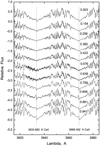 |
Fig. 2 Same as Fig. 1 but for H and Κ Ca II lines (their position is indicated by vertical dashed lines). |
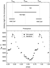 |
Fig. 4 Schematic visualisation of the appearance and disappearance of chromosphere emissions in X Cyg, accompanied by a graph of the effective temperature variation of this star with the pulsation phase. Literature data on effective temperature are from Luck (2018). Vertical lines indicate the moments of the maximum and minimum radius of the star. |
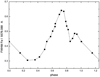 |
Fig. 5 Behaviour of the FWHM Fe II line 5576.088 Å in the X Cyg spectra. |
4 Some UV and IR chromosphere indicators: the NLTE consideration
In this paper, we also extended our NLTE consideration of the He I triplet formation using data for two additional phases where the emission in this triplet is clearly visible. The same method as in the NLTE analysis of Kovtyukh et al. (2022) was applied for one phase.
In modelling the emission in the He I 10 830 Å line, we considered the effect of departure from local thermodynamical equilibrium (NLTE effects) on the calculated spectrum. Our NLTE model consists of 55 He I atomic levels and the He II ground level, which are considered in detail. The model was described in Korotin & Ryabchikova (2018). To find the level populations, we applied the MULTI code by Carlsson (1986), with slight modifications (Korotin et al. 1999).
We attempted a very simple simulation of the X Cyg chromosphere at the pulsation phases 0.422, 0.576, and 0.638, where the helium emission is well observed (the very preliminary result was also reported in Kovtyukh et al. 2022 for phase 0.422). For this purpose, we set the linear temperature rise in the chromosphere as a function of the logarithm of the mass number, namely, Τ = Tmin+slopeilog(mmin) − log(m)). The point of the temperature minimum was selected as a starting point of the chromosphere temperature rise. Thereafter, in this primitive chromosphere, we calculated the electron concentration and gas pressure using the ATLAS9 code (Castelli & Kurucz 2003). The slope of the temperature distribution as a function of height in the chromosphere was selected empirically by comparing the observed and calculated helium emissionline profiles.
Several variants of the chromosphere were considered, each with a different temperature minimum position. The slope of the temperature distribution significantly affects the emission strength. When the slope is small, the emission is either not seen at all, or a line appears in absorption. With increasing slope, the absorption profile changes to emission. The higher in the envelope the temperature minimum is located, the larger the slope value must be to cause helium emission. Together with the intensity of the emission, the profile width also changes.
It should be noted that in all of the cases considered, the core of the helium line is formed at temperatures of about 12 000–15000 Κ and an electronic concentration of about 1010 cm−3. Relatively good agreement is seen between the observed and calculated profiles if we use a chromosphere model with Tmin in the range 2700–2900 K, log(mmin) in the range between −1.6 and −1.4 dex, and with a slope between 41 000 and 37 000 Κ log(m)−1 (see Fig. 6). The synthetic spectra were produced with the help of the SynthV code of Tsymbal et al. (2019) with helium line profiles computed in NLTE (using the level populations obtained with MULTI) and profiles of other lines synthesised in LTE. Atomic line data for these lines treated in LTE were taken from the VALD3 database (Ryabchikova et al. 2015). How the emission profile changes with the adopted chromosphere parameters is illustrated in Fig. 7.
We also applied our simple consideration to investigate UV doublets of Ca II and Mg II, and the IR triplet of Ca II. For this purpose, we used our calcium atomic model and the methods described in Spite et al. (2012) and Caffau et al. (2019). Our model of Ca atom consists of 70 levels of Ca I, 38 levels of Ca II, and the ground state of Ca III. In addition, more than 300 levels of Ca I and Ca II were included in consideration in order to preserve the condition of the particle number conservation in LTE. We used the Mg I atomic model described in Mishenina et al. (2004), and later modified by Cerniauskas et al. (2017) to calculate the magnesium line profiles. This model was then supplemented with five levels of Mg II ion and the ground level of Mg III. The corresponding transitions between the added levels were taken into account. In a first approximation, this model allowed us to estimate the emissions in the resonant doublet Mg II lines and determine their approximate localisation.
Figure 8 demonstrates the adopted temperature distributions in the chromosphere at two phases: 0.422 and 0.848. At phase 0.422, the effective temperature is lower than at phase 0.848. The cores of the UV Ca II doublet lines on phases used to describe the helium lines are formed below the layer of the temperature minimum, and there is no emission. The 'calcium' chromosphere is thin in the mass scale. At the phase 0.848, the line cores are formed well above the temperature minimum; the calcium chromosphere is expanded, and these conditions lead to the appearance of emission. Therefore, to visualise the above discussion in Fig. 8, only two phases were chosen.
Our calculations show that including the chromosphere temperature rise at the phases between 0.4 and 0.6 does not cause any emission appearance in the IR calcium triplet. This is in complete agreement with observational data reported by Wallerstein et al. (2019) for X Cyg at these phases. However, judging from the profiles shown in Fig. 12 of Wallerstein et al. (2019), one can note emission at the phases of about 0.7. According to Martin et al. (2017), the IR Ca II triplet emission correlates with UV Ca II H and Κ emission. We should note here that these latter authors considered only F to Κ main sequence stars that have more or less 'stationary' chromospheres. We emphasise that it is possible that emission in the IR Ca II triplet may be present also in other phases, but as we do not have the original spectra at our disposal, and therefore we have to rely only on the processed data and the resulting profiles presented in Fig. 12, we cannot draw any definite conclusion about such a possibility and therefore leave this question open.
Our NLTE calculations for the UV Mg II doublet lines led us to conclude that the emission is present at all phases. Unfortunately, our calculated NLTE profiles show extremely strong emissions, which contradicts the observations, and therefore they cannot be considered real. It may not be possible to correctly describe the magnesium doublet emissions with the NLTE model of this ion that we currently have at our disposal, and with the very simplified 'chromosphere model'. The problem is less severe for the calcium doublet, but it also exists.
In summary, we conclude that the Cepheid chromospheres differ from the stationary chromospheres of the non-variable supergiants of the same spectral type. Large-scale dynamic phenomena in the Cepheid envelopes caused by propagating shock waves make the chromosphere extremely inhomogeneous in temperature and density, meaning that these characteristics are a function of the height above the photosphere and time. This leads to the appearance and disappearance of emissions in the different chromosphere indicators in different pulsation phases.
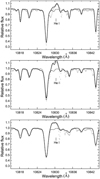 |
Fig. 6 Observed and synthesised spectra of X Cyg in the vicinity of the helium IR lines at pulsation phases 0.422, 0.576, and 0.638. Open circles represent observed fragments of the spectra. The continuous line shows our synthetic spectrum with an account of the chromosphere emission, while the dashed line represents the synthetic spectrum, ignoring the chromosphere. |
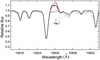 |
Fig. 7 Changes in the synthetic emission profile at phase 0.638. The blue solid line shows the case of increasing the temperature slope by 1000 K, while the blue dashed line shows the case of a decrease in slope by 1000 K. The red solid line shows the position of the temperature minimum in the mass coordinate, increased by 0.04 dex, while the red dashed line shows its decrease by 0.04 dex. The other designations are the same as in Fig. 6. |
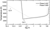 |
Fig. 8 Two adopted chromosphere models that describe the behaviour of the UV Ca II doublet lines at phases 0.422 and 0.848. |
5 Conclusion
In summary, we considered UV emissions in Ca II and Mg II lines, as well as novel detections of IR emission in the He I 10 830 Å line in X Cyg spectra. We believe that the UV emissions considered, which are observed at phases before maximum light (Ca II) and approximately between maximum and minimum light (Mg II) can be explained within the phenomenological Gillet (2014) shock-wave model. This model considers the simultaneous presence in the X Cyg shell of at least two shock waves. One is the main shock wave, and the other is the shock originating from the previous pulsating cycle. The latter has already detached from the photosphere and is propagating in the higher layers. The IR redshifted He I emission is excited in the upper(most) layers of the star's envelope, in its falling layers. This occurs in the time interval between the maximum and pre-minimum of the radius (see Engle et al. 2017, Fig. 1, but for classical Cepheid δ Cep, or the radial velocity curves; see Wallerstein et al. 2019 for X Cyg itself).
The emission-forming layers are falling with relatively low acceleration toward the star, and the emission itself exists for about 10 days. At these phases, Engle et al. (2017) also report X-ray emission (see Sect. 1), which must be excited in the upper layers of the Cepheid shell. We note, that there may well be a phase shift (positive or negative) between the Gillet (2014) model prediction and the time of appearance and disappearance of Ca II and Mg II emissions, because the model is based on the behaviour of the Hα line only.
We emphasise that our modelling results are estimates and should be taken with caution, because several possible important factors were ignored in our simple consideration (e.g. X-ray inward radiation from the corona; possible computational uncertainties in the ionisation equilibrium condition; and, perhaps, the far-from-realistic assumed linear temperature growth in the 'chromosphere'). Nevertheless, we consider this only a first step in quantifying the process of the emission generation in the IR He II 10 830 Å triplet in such pulsating variables as classical Cepheids.
Acknowledgements
S.M.A. and V.V.K. are grateful to the Vector-Stiftung at Stuttgart, Germany, for support within the program "2022 – Immediate help for Ukrainian refugee scientists" under grants P2022-0063 and P2022-0064. Especial thanks to Prof. K. Werner and Dr. V. Suleimanov for their help with organising our stay in the Institute of Astronomy and Astrophysics of the Tübingen University. The authors are grateful to Dr. N. Nardetto, whose spectra from the observational program formed the basis for the preparation of this paper. The IUE browse files were conceived and originally implemented by Dr. Derck Massa, Dr. Nancy Oliversen, and Ms. Patricia Lawton, then members of the GSFC Astrophyics Data Facility (ADF) staff under direction of Dr. Michael Van Steenberg. Some modifications have been made as part of the transition to MAST maintenance. We are extremely grateful to our anonymous referee, who analyzed the manuscript in depth and gave us very important suggestions that improved the text, making it more understandable to the reader.
References
- Adams, W. S., & Joy, A. H. 1939, PASP, 9, 254 [Google Scholar]
- Andrievsky, S. M., & Garbuzov, G. A. 1991, Mechanisms of Chromospheric and Coronal Heating, Proceedings of the International Conference, eds. P. Ulmschneider, E. R. Priest & R. Rosner (Springer-Verlag), 356 [CrossRef] [Google Scholar]
- Andrievsky, S. M., & Garbuzov, G. A. 1992/1993, Odessa Astron. Publ., 6, 31 [Google Scholar]
- Andrievsky, S. M., & Matveev, I. A. 1991, Ap, 35, 312 [NASA ADS] [Google Scholar]
- Andrievsky, S. M., Garbuzov, G. A., & Savanov, I. S. 1987, Stellar Atmospheres Conference Proceedings, Odessa National University, 153 [Google Scholar]
- Beigman, I. L., & Stepanov, A. E. 1981, Pis’ma Astron. Zh., 7, 172 [Google Scholar]
- Bonnell, J. T., & Bell, R. A. 1985, PASP, 97, 236 [CrossRef] [Google Scholar]
- Böhm-Vitense, E., & Dettmann, T. 1980, ApJ, 236, 560 [CrossRef] [Google Scholar]
- Böhm-Vitense, E., & Parsons, S. B. 1983, ApJ, 266, 171 [CrossRef] [Google Scholar]
- Caffau, E., Monaco, L., Bonifacio, P., et al. 2019, A&A, 628, A46 [NASA ADS] [CrossRef] [EDP Sciences] [Google Scholar]
- Carlsson, M. 1986, Upps. Astron. Obs. Rep., 33 [Google Scholar]
- Castelli, F., & Kurucz, R. L. 2003, IAU Symp., 210, A20 [Google Scholar]
- Černiauskas, A., Kučinskas, A., Klevas, J., et al. 2017, A&A, 604, A35 [Google Scholar]
- Engle, S. G., & Guinan, E. F. 2012, J. Astron. Space Sci., 29, 181 [NASA ADS] [CrossRef] [Google Scholar]
- Engle, S. G., Giunan, E. F., Harper, G. M., Neilson, H. R., & Evans, N. R. 2014, ApJ, 794, 80 [NASA ADS] [CrossRef] [Google Scholar]
- Engle, S. G., Giunan, E. F., Harper, G. M., et al. 2017, ApJ, 838, 67 [NASA ADS] [CrossRef] [Google Scholar]
- Evans, N. R., Guinan, E., Engle, S., et al. 2010, AJ, 139, 1968 [NASA ADS] [CrossRef] [Google Scholar]
- Evans, N. R., Pillitteri, I., Kervella, P., et al. 2021, ApJ, 162, 92 [CrossRef] [Google Scholar]
- Fadeyev, Y. A., & Gillet, D. 1998, A&A, 333, 687 [NASA ADS] [Google Scholar]
- Fadeyev, Y. A., Le Coroller, H., & Gillet, D. 1998, A&A, 392, 735 [Google Scholar]
- Fokin, A. B. 1991, MNRAS, 250, 258 [NASA ADS] [CrossRef] [Google Scholar]
- Fokin, A. B. 1992, MNRAS, 256, 26 [NASA ADS] [CrossRef] [Google Scholar]
- Fokin, A. B., Gillet, D., & Breitfellner, M. G. 1996, A&A, 307, 503 [NASA ADS] [Google Scholar]
- Fracassini, M., & Pasinetti, L. E. 1982, A&A, 107, 326 [NASA ADS] [Google Scholar]
- Fracassini, M., Pasinetti, L. E., Castelli, F., Antonello, E., & Pastori, L. 1983, ApJS, 97, 323 [Google Scholar]
- Fracassini, M., Pasinetti Fracassini, L. E., Pastori, L., Teays, T. J., & Mariani, A. 1991, A&A, 243, 458 [NASA ADS] [Google Scholar]
- Garbuzov, G. A., & Andrievsky, S. M. 1986, Astrophysics, 25, 498 [Google Scholar]
- Gieren, W. P., Moffet, T. J., & Barnes III, T. G. 1999, ApJ, 512, 553 [NASA ADS] [CrossRef] [Google Scholar]
- Gillet, D. 2014, A&A, 568, A72 [NASA ADS] [CrossRef] [EDP Sciences] [Google Scholar]
- Gillet, D., & Fokin, A. B. 2014, A&A, 565, A73 [NASA ADS] [CrossRef] [EDP Sciences] [Google Scholar]
- Gratton, L. 1953, ApJ, 118, 570 [NASA ADS] [CrossRef] [Google Scholar]
- Hill, S. J. 1972, ApJ, 178, 793 [Google Scholar]
- Hillendahl, R. W. 1970, PASP, 82, 1231 [NASA ADS] [CrossRef] [Google Scholar]
- Hintz, E., Harding, T. B., & Hintz, M. L. 2021, AJ, 162, 149 [NASA ADS] [CrossRef] [Google Scholar]
- Hocdé, V., Nardetto, N., Borgniet, S., et al. 2020, A&A, 641, A74 [EDP Sciences] [Google Scholar]
- Hocdé, V., Nardetto, N., Matter, A., et al. 2021, A&A, 651, 92 [Google Scholar]
- Hollars, D. R. 1974, ApJ, 194, 137 [NASA ADS] [CrossRef] [Google Scholar]
- Joy, A. H., & Wilson, R. E. 1949, ApJ, 109, 231 [NASA ADS] [CrossRef] [Google Scholar]
- Kiss, L. 1998, MNRAS, 297, 825 [NASA ADS] [CrossRef] [Google Scholar]
- Korotin, S. A., & Ryabchikova, T. A. 2018, AstL, 44, 621 [NASA ADS] [Google Scholar]
- Korotin, S. A., Andrievsky, S. M., & Luck, R. E. 1999, A&A, 351, 168 [NASA ADS] [Google Scholar]
- Kovtyukh, V. V., Wallerstein, G., Andrievsky, S. M., et al. 2011, A&A, 526, A116 [NASA ADS] [CrossRef] [EDP Sciences] [Google Scholar]
- Kovtyukh, V. V., Andrievsky, S. M., & Korotin, S. A. 2022, MNRAS 517, L143 [CrossRef] [Google Scholar]
- Kraft, R. P. 1957, ApJ, 125, 336 [NASA ADS] [CrossRef] [Google Scholar]
- Luck, R. E. 2018, AJ, 156, 171 [Google Scholar]
- Martin, J., Fuhrmeister, B., Mittag, M., et al. 2017, A&A, 605, A113 [NASA ADS] [CrossRef] [EDP Sciences] [Google Scholar]
- Mathias, P., Gillet, D., Fokin, A. B., et al. 2006, A&A, 457, 575 [CrossRef] [EDP Sciences] [Google Scholar]
- Mishenina, T. V., Soubiran, C., Kovtyukh, V. V., & Korotin, S. A. 2004, A&A, 418, 551 [NASA ADS] [CrossRef] [EDP Sciences] [Google Scholar]
- Moschou, S.-P., Vlahakis, N., Drake, J. J., et al. 2020, ApJ, 900, 157 [NASA ADS] [CrossRef] [Google Scholar]
- Nardetto, N., Groh, J. H., Kraus, S., et al. 2008, A&A, 489, 1263 [NASA ADS] [CrossRef] [EDP Sciences] [Google Scholar]
- O’Brien, G. T., & Lambert, D. L. 1986, ApJS, 62, 899 [NASA ADS] [CrossRef] [Google Scholar]
- Oskinova, L. M., Nazé, Y., Todt, H., et al. 2014, Nat. Commun., 5, 4024 [CrossRef] [Google Scholar]
- Parsons, S. B. 1980, ApJ, 239, 555 [NASA ADS] [CrossRef] [Google Scholar]
- Parthasarathy, M., & Parsons, S. B. 1984, NASA. Goddard Space Flight Center Future of Ultraviolet Astronomy Based on Six Years of IUE Research, 342, SEE N85-20961, 11 [Google Scholar]
- Ryabchikova, T., Piskunov, N., Kurucz, R. L., et al. 2015, Phys. Scr, 90, 054005 [Google Scholar]
- Sasselov, D. D., & Lester, J. B. 1994a, ApJ, 423, 777 [NASA ADS] [CrossRef] [Google Scholar]
- Sasselov, D. D., & Lester, J. B. 1994b, ApJ, 423, 785 [NASA ADS] [CrossRef] [Google Scholar]
- Sasselov, D. D., & Lester, J. B. 1994c, ApJ, 423, 795 [NASA ADS] [CrossRef] [Google Scholar]
- Schmidt, E. G., & Parsons, S. B. 1982a, ApJS, 48, 185 [NASA ADS] [CrossRef] [Google Scholar]
- Schmidt, E. G., & Parsons, S. B. 1982b, in Advances in Ultraviolet Astronomy: Four Years of IUE Research, eds. Y. Kondo, J. Mead, & R. Chapman, NASA Conf. Pub., 2238, 439 [NASA ADS] [Google Scholar]
- Schmidt, E. G., & Parsons, S. B. 1984a, ApJ, 279, 202 [NASA ADS] [CrossRef] [Google Scholar]
- Schmidt, E. G., & Parsons, S. B. 1984b, ApJ, 279, 215 [NASA ADS] [CrossRef] [Google Scholar]
- Schmidt, E. G., & Weiler, E. J. 1979, AJ, 84, 231 [NASA ADS] [CrossRef] [Google Scholar]
- Spite, M., Andrievsky, S. M., Spite, F., et al. 2012, A&A, 541, A143 [NASA ADS] [CrossRef] [EDP Sciences] [Google Scholar]
- Szabados, L. 1991, Commun. Konkoly Obs., XI, 123 [NASA ADS] [Google Scholar]
- Teays, T. J., Schmidt, E. G., Fracassini, M., & Pasinetti Fracassini, L. E. 1989, ApJ, 343, 916 [NASA ADS] [CrossRef] [Google Scholar]
- Tsymbal, V., Ryabchikova, T., & Sitnova, T. 2019, ASP Conf. Ser., 518, 247 [NASA ADS] [Google Scholar]
- Van Hoof, A. 1948, ApJ, 108, 160 [NASA ADS] [CrossRef] [Google Scholar]
- Wallerstein, G., Anderson, R. I., Farrell, E. M., et al. 2019, PASP, 131, 094203 [CrossRef] [Google Scholar]
- Zirin, H. 1975, ApJ, 199, L63 [NASA ADS] [CrossRef] [Google Scholar]
All Figures
|
Fig. 1 Emission in the IR triplet in the spectra of X Cyg. Vertical dashed lines indicate phases with emission. Hereinafter, the phases are calculated according to Hintz et al. (2021). |
| In the text | |
|
Fig. 2 Same as Fig. 1 but for H and Κ Ca II lines (their position is indicated by vertical dashed lines). |
| In the text | |
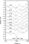 |
Fig. 3 Same as Fig. 1 but for h and k Mg II lines. |
| In the text | |
|
Fig. 4 Schematic visualisation of the appearance and disappearance of chromosphere emissions in X Cyg, accompanied by a graph of the effective temperature variation of this star with the pulsation phase. Literature data on effective temperature are from Luck (2018). Vertical lines indicate the moments of the maximum and minimum radius of the star. |
| In the text | |
|
Fig. 5 Behaviour of the FWHM Fe II line 5576.088 Å in the X Cyg spectra. |
| In the text | |
|
Fig. 6 Observed and synthesised spectra of X Cyg in the vicinity of the helium IR lines at pulsation phases 0.422, 0.576, and 0.638. Open circles represent observed fragments of the spectra. The continuous line shows our synthetic spectrum with an account of the chromosphere emission, while the dashed line represents the synthetic spectrum, ignoring the chromosphere. |
| In the text | |
|
Fig. 7 Changes in the synthetic emission profile at phase 0.638. The blue solid line shows the case of increasing the temperature slope by 1000 K, while the blue dashed line shows the case of a decrease in slope by 1000 K. The red solid line shows the position of the temperature minimum in the mass coordinate, increased by 0.04 dex, while the red dashed line shows its decrease by 0.04 dex. The other designations are the same as in Fig. 6. |
| In the text | |
|
Fig. 8 Two adopted chromosphere models that describe the behaviour of the UV Ca II doublet lines at phases 0.422 and 0.848. |
| In the text | |
Current usage metrics show cumulative count of Article Views (full-text article views including HTML views, PDF and ePub downloads, according to the available data) and Abstracts Views on Vision4Press platform.
Data correspond to usage on the plateform after 2015. The current usage metrics is available 48-96 hours after online publication and is updated daily on week days.
Initial download of the metrics may take a while.