| Issue |
A&A
Volume 670, February 2023
|
|
|---|---|---|
| Article Number | A26 | |
| Number of page(s) | 12 | |
| Section | Planets and planetary systems | |
| DOI | https://doi.org/10.1051/0004-6361/202244180 | |
| Published online | 01 February 2023 | |
Occurrence rate of hot Jupiters orbiting red giant stars
Leiden Observatory, Leiden University,
Postbus 9513,
2300 RA,
Leiden, The Netherlands
e-mail: This email address is being protected from spambots. You need JavaScript enabled to view it.
Received:
3
June
2022
Accepted:
1
December
2022
Abstract
Context. Hot Jupiters form an enigmatic class of object whose formation pathways are not yet clear. Determining their occurrence rates as a function of orbit, planet and stellar mass, and system age can be an important ingredient for understanding how they form. To date, various hot Jupiters have been discovered orbiting red giant stars, and deriving their incidence would be highly interesting.
Aims. In this study our aim is to determine the number of hot Jupiters in a well-defined sample of red giants, estimate their occurrence rate, and compare it with that for A-, F-, and G-type stars.
Methods. A sample of 14474 red giant stars, with estimated radii between 2 and 5 R⊙, was selected using Gaia to coincide with observations by the NASA TESS mission. Subsequently, the TESS light curves were searched for transits from hot Jupiters. The detection efficiency was determined using injected signals, and the results further corrected for the geometric transit probability to estimate the occurrence rate.
Results. Three previously confirmed hot Jupiters were found in the TESS data, in addition to one other TESS object of interest, and two M-dwarf companions. This results in an occurrence rate of 0.37−0.09+0.29%. Due to the still large uncertainties, this cannot be distinguished from that of A-, F-, and G-type stars. We argue that it is unlikely that planet engulfment in expanding red giants plays an important role in this sample.
Key words: planets and satellites: detection / planets and satellites: dynamical evolution and stability / planets and satellites: gaseous planets / stars: evolution
© The Authors 2023
 Open Access article, published by EDP Sciences, under the terms of the Creative Commons Attribution License (https://creativecommons.org/licenses/by/4.0), which permits unrestricted use, distribution, and reproduction in any medium, provided the original work is properly cited.
This article is published in open access under the Subscribe-to-Open model. This email address is being protected from spambots. You need JavaScript enabled to view it. to support open access publication.
1 Introduction
Hot Jupiters (HJs) are very interesting objects to study. The close proximity to their host stars makes them perfect candidates to observe with the transit method and causes their atmospheres to reach temperatures that are similar to some M-dwarf stars. However, it is still unknown how these objects form. To date, various hypotheses have been developed that could possibly explain their formation. The most promising are in situ formation, disk migration, and high-eccentricity tidal migration (Dawson & Johnson 2018).
One possible way to gain more information on the formation and the evolution of HJs is through the study of the occurrence rates as a function of planet and stellar masses, orbits, and system ages. Zhou et al. (2019) determined the HJ occurrence rate to be 0.43 ± 0.15 and 0.71 ± 0.31% for F- and G-type stars, respectively, while that around Kepler stars was estimated to be 0.43 ± 0.05 (Fressin et al. 2013),  (Masuda & Winn 2017), and
  (Petigura et al. 2018). Zhou et al. (2019) found the occurrence rate around A stars to be 0.26 ± 0.11. Furthermore, Grunblatt et al. (2019) estimated the occurrence rate of giant planets around low-luminosity red giants to be 0.51 ± 0.29%.
It is particularly interesting to determine the occurrence rate of HJs around red giant stars. As evolved stars have gone through their initial hydrogen core burning phase, an estimate for the occurrence rate of HJs may tell us more about the evolution of these planetary systems and the survivability of close-in planets. To date, various HJs have been found to orbit red giants, Kepler-91b (Lillo-Box et al. 2014) being one of the most prominent.
In addition to HJs other kinds of exoplanetary populations have been found orbiting red giant stars as well. For example, both hot Neptune (e.g. K2-39b; Van Eylen et al. 2016) and warm eccentric Jupiter (e.g. Kepler-432b; Ciceri et al. 2015; Quinn et al. 2015) subpopulations have also been found. In addition, the detections of Kepler-56 b and c have shown that red giants can contain multiplanetary systems (Borucki et al. 2011; Huber et al. 2013).
In this paper we estimate the occurrence rate of HJs around red giants. In Sect. 2 we describe how we created a well-defined sample of red giants in the solar neighbourhood observed by the NASA TESS mission. In Sect. 3 we explain how we searched for HJs transiting these stars. Section 4 describes how we estimated the occurrence rate of HJs around red giants by combining the geometric probability of observing transits and the fraction of detected HJs. Our discussion and conclusions can be found in Sect. 5.
2 Sample selection and TESS observations
2.1 Gaia sample of red giant stars
All stars with available photometric measurements in the G, GBP, and GRP passbands, with estimated absolute magnitudes of MG ≤ 5.5 and with parallaxes of ϖ ≥ 2 milliarcseconds were selected using the Gaia DR2 catalogue (Gaia Collaboration 2016). To ensure that the sample contained only stars with sufficiently precise photometric and astrometric properties, the sample was subject to the following selection criteria, similar to those imposed in Gaia Collaboration (2018):
First we remove all the stars with high astrometric excess noise by imposing the constraint
 (1)
(1)
where χ2 is the ASTROMETRIC_CHI2_AL parameter and v’ is the ASTROMETRIC_N_GOOD_OBS_AL parameter. The values for χ2 and v′ were obtained from the Gaia DR2 catalogue. Next, to be able to correctly estimate the absolute magnitudes, we only retained the stars which have a precision of at leat 10% on their measured parallax,
 (2)
(2)
To only have stars in the sample with accurate photometric quantities, we imposed the following constrains on the signal-to-noise in the different Gaia passbands:
 (3)
(3)
As the Gaia GBP and GRP passbands were not corrected for blending of background sources. We remove the stars in our sample whose fluxes might suffer from contamination from background sources, all stars with PHOT_BP_RP_EXCESS_FACTOR  falling outside the following two limits were removed from the collection:
 (4)
(4)
Finally, we only retained the stars with well-measured astrometric quantities and remove those with a renormalised unit weight error of above 1.4.
We reduced the sample further by ensuring that all stars had been observed during the first two years of TESS observations and for which it is expected that transits can be detected. First, we used the Python package TESS-POINT was used to check if the stars, based on their positional coordinates (right ascension and declination), are located in one of the first 26 TESS sectors. Next, we imposed an upper limit of R ≤ 10 R⊙ on the stellar radii, as the transit depth scales inversely with the stellar radius squared. Furthermore, a lower limit of R ≥ 2 R⊙ was imposed as we assumed this to be the typical stellar radius at the base of the red giant branch (RGB). Finally, we only retained the stars with apparent magnitudes of T ≤ 10, as the transit signals might be lost in the noise of the lightcurves of faint stars. The apparent magnitudes were estimated using Eq. 1 of Stassun et al. (2019):
 (5)
(5)
Finally, stars were selected based on their position in the colour–magnitude diagram (CMD) to remove stars from the sample that do not reside on the RGB. This criterion ensures that massive subgiant stars of similar radii do not contaminate the sample of red giant stars. The selection region has the following boundaries:
 (6)
(6)
The resulting CMD of the stars surviving the imposed selection criteria, together with the selection boundaries, is displayed in Fig. 1. The final sample consisted of 35 250 red giants.
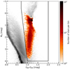 |
Fig. 1 Colour-magnitude diagram of stars that have survived the imposed selection criteria. The black box represents the boundaries of the region enclosing the RGB. The colour (GBP − GRP) of the stars can be found on the x-axis, while the y-axis denotes the absolute magnitudes. The logarithmic colour map indicates the number of stars in each two-dimensional bin. Stars removed by the selection criteria are shown in grey. |
2.2 TESS observations
If available, the two-minute cadence TESS Pre-search Data Condition SAP (PDCSAP; Jenkins et al. 2016) light curves were downloaded, otherwise the light curves were extracted from the 30-minute full frame images (FFIs) using the python package TESSERACT1. About 83% of the light curves were obtained using TESSERACT and all these light curves were obtained using the default aperture option, which is based on the K2P2 method (see Lund et al. 2015).
The baselines of the light curves were detrended using an iterative spline fitting method (Vanderburg & Johnson 2014). The splines consisted of polynomials of degree 3, and in each iteration we excluded the 3σ outliers until no outliers remained. We further cleaned the light curves by removing all data points lying 3σ above the detrended baselines. Following Vanderburg et al. (2016), the two lowest data points were removed as well.
3 BLS search for hot Jupiters
To search the cleaned light curves for transits arising from HJ candidates on periods between 4 and 25 days, we used the BoxLeastSquares (BLS) implementation of the python package ASTROPY (Astropy Collaboration 2013, 2018). The periodograms, yielded by the BLS method, were normalised following the steps given in Vanderburg et al. (2016). First, we subtracted the changing baseline level of the periodograms, to avoid spurious detections at longer periods. Next, we converted the BLS power measurements to signal-to-noise ratios by using Eq. 4 of Vanderburg et al. (2016),
 (7)
(7)
Here MAD stands for the median absolute deviation.
To validate any signals arising in the normalised periodograms, the periodograms were subject to a self-imposed algorithm, consisting of the following steps: first, we set a limit of S/N ≥ 9 on the highest peak found in the periodogram. If the highest peak did not meet this limit, it was assumed that the light curve did not contain any transits. Subsequently, the algorithm would consider the combination of transit parameters (orbital period, midpoint of first transit, transit depth, and transit duration) belonging to the signal yielding the highest peak in periodogram.
Secondly, if the corresponding transit duration was found to be longer than 25% of the orbital period, the found signal was rejected. If only a single data point was found in the fitted boxes of the BLS method, the signal was considered to be a false positive. In these cases, the algorithm would remove the data points yielding the signal from the light curves, generate a new periodogram, and return to step 1.
Finally, the radius of the candidate was estimated using
 (8)
(8)
where ∆F is the transit depth and R is the stellar radius. The candidate was assumed to be a potential HJ if R ≤ 2.2 RJup.
The periodograms that passed all the steps were subsequently subjected to an individual visual inspection. The visual inspection allowed us to distinguish between real candidates and false positives. Among the false positives, we included binary stars, features in the light curves that clearly did not have a transit shape, and objects that were found to transit background stars. The objects orbiting background stars were investigated by thoroughly studying the TESS target pixel files.
3.1 Transit search results
The search for HJ candidates lead to 1392 potential detections, of which all except 6 were rejected upon visual inspection. The other 1386 detections were found to be false positives, binary stars, or objects orbiting stars in the background of the target star. The objects orbiting background stars were found by thoroughly studying the TESS target-pixel files and the light curves associated with each pixel.
The potential candidates were found orbiting the stars CD-25 2180, HD 1397, HD 93396 (also known as KELT-11), HD 221416, TYC 4004-1837-1, and TYC 5456-76-1. A literature study revealed that the candidates orbiting HD 1397, KELT-11, and HD 221416 correspond to the already confirmed exoplanets HD 1397b (Nielsen et al. 2019), KELT-11b (Pepper et al. 2017), and HD 221416b (Huber et al. 2019). The candidate orbiting the star TYC-5456-76-1 was found to correspond to the TESS object of interest TOI-2669.01, and the planetary nature of this candidate has recently been confirmed by Grunblatt et al. (2022). The final two candidates orbiting CD-25 2180 and TYC-4004-1837-1 were found to be M-dwarf stellar companions, using existing radial velocity measurements.
As mentioned before, 83% of the light curves were obtained using TESSERACT. The light curves of TYC-5456-76-1, CD-25 2180, and both light curves of TYC-4004-1387-1 were obtained using TESSERACT. The light curves of KELT-11 and HD 221416 were both obtained from the Science Processing Operations Center (SPOC) pipeline, while one of the light curves of HD 1397 was obtained using the SPOC pipeline (sector 1) and the other using TESSERACT (sector 2). As the two pipelines resulted in similar numbers of observed candidates, both pipelines appear to reach similar sensitivities.
Distributions and hyperparameters used during the GP method.
A priori parameter limits used in the MCMC algorithm.
3.2 Fitting the transits
To extract as much information about the found objects and their orbits, we fitted a transit model to the light curves using a Markov chain Monte Carlo (MCMC) algorithm, using the Python package EMCEE (Foreman-Mackey et al. 2013). The light curves were first re-detrended using a Gaussian processes (GP) method, which was implemented using the JULIET package (Espinoza et al. 2019). To ensure that the transit would not influence the GP trend, the out-of-transit data was removed by phase-folding the light curves, based on the period and midpoint of first transit found with our BLS search, and excluding all points that fall within 0.02 of the absolute phases. Subsequently, the GP trend was determined using the default Matern kernel; the hyperparameters used can be found in Table 1. The detrended light curves can be found in Appendix A.
The model light curves were created using the Python package PYTRANSIT (Parviainen 2015), assuming for simplicity linear limb-darkening with a value of 0.5 and circular orbits. The remaining parameters (orbital period, midpoint of first transit, ratio of object radius to stellar radius, semi-major axis in stellar radii, and inclination) were fitted with the MCMC algorithm. The a priori distributions for the various parameters are in Table 2. The best fitting transit models and the corresponding values for the transit parameters can be found in Appendix B.
4 Occurrence rate
To estimate the occurrence rate of HJs around red giants, we derived the geometric probability and the probability of actually detecting transits of the planets as functions of orbital period and planetary and stellar sizes.
4.1 Geometric probability
The geometric probability is the probability of observing a transit in a randomly oriented system. It depends mostly on the ratio of the semi-major axis of the orbit (a) to the stellar radius. The geometric probability can be calculated using Eq. 2 in Kipping (2014),
 (9)
(9)
where after the right-hand equal sign, for simplicity the orbits are assumed to be circular by setting the eccentricity to e = 0 (see Table 3).
For our occurrence rate estimate, we used the average geometric probability of  .
.
Stellar masses, stellar radii, planetary radii, planetary masses, and semi-major axes used in the calculation for the geometric probability.
4.2 Observational probability
To estimate the fraction of HJs detected, we performed artificial injection tests. The injected transits were based on the orbit of Kepler-91b (Lillo-Box et al. 2014). We carried out the injection tests for planetary radii of Rp = 1.0 RJup, 1.5 RJup, and 2.0 RJup, assuming an inclination of 90%. Our injected planets have periods between 4 and 15 days, randomly picked from a log-normal distribution. This period range covers the same range as for the detected planets in the geometric probability. For each planetary radius we conducted five different tests, where in each test 150 stars were randomly chosen from our sample of red giants. Figure 2 shows the number of correctly detected and non-detected injected transits (top row), with the percentages of the correctly detected transits (bottom row).
As the confirmed exoplanets all orbit red giants with stellar radii of R < 5 R⊙, we only focus on these stellar radii in our calculation for the observational probability to ensure that both geometric and observational probabilities account for a similar population of red giant stars. This means that in the subsequent calculation of the total occurrence rate, we will only consider the 14 474 stars in our sample with radius R < 5 R⊙. To account for the fact that a greater number of smaller HJs with radii 1.0 RJup ≤ R ≤ 1.5 RJup have been observed than the larger HJs (R > 1.5 RJup), we have added weights based on the observed HJs with radii 1.0 RJup ≤ R ≤ 2.0 RJup and orbital periods P ≤ 15 days2.
We acquired a total number of 501 observed HJs, of which 323 have radii between 1.0 RJup ≤ R ≤ 1.33 RJup, 136 have radii between 1.33 RJup ≤ R ≤ 1.66 RJup and 42 have radii between 1.66 RJup ≤ R ≤ 2.0 RJup. Based on these values, we establish that about two times more HJs have radii close to 1.0 RJup compared to 1.5 RJup and three times more HJs have radii close to 1.5 RJup compared to ~2.0 RJup. Subsequently, we determined our fraction of observed HJs using a weighted average, where we used weights of 2, 1, and  , respectively. Our weighted averaged yields a percentage of 0.38 ± 0.13 detected HJs.
4.3 Total probability and occurrence rate
Combining the geometric and detection probability, we find the combined probability of seeing a HJ with our method to be 0.07 ± 0.03. In our search for HJs orbiting red giants, we find four systems. Correcting for the geometric probability and detection fraction, we estimate that there are 40–96 planets orbiting our sample stars. For our sample of 14474 red giants with R ≤ 5 R⊙, this yields an occurrence rate of  .
.
5 Discussion
5.1 Occurrence rate
The occurrence rate derived here of  agrees, within the uncertainties, with those for the A-, F-, and G-type stars of, respectively, 0.26 ± 0.11, 0.43 ± 0.15, and 0.71 ± 0.31% (Zhou et al. 2019). These occurrence rates were derived for HJs with orbital periods between 0.9 and 10 days. No clear distinction can yet be made between the occurrence rates of these different stellar types. The occurrence rate also agrees with that for HJs orbiting the Kepler stars of 0.43 ± 0.05% (0.8 ≤ P ≤ 10 days; Fressin et al. 2013),
  (P ≤ 10 days Masuda & Winn 2017), and
  (1 ≤ P ≤ 10 days Petigura et al. 2018). Finally, our found value is similar to that reported by Grunblatt et al. (2019) for giant planets orbiting low-luminosity red giants (P ≤ 10 days) in the K2 observations, 0.51 ± 0.29%. All in all, the found occurrence rate for HJs orbiting red giant stars cannot (yet) be distinguished from the occurrence rates reported for the above-mentioned stellar types.
The masses of the three host stars already discussed in the literature are estimated to be in the range 1.2–1.5 M⊙, meaning that they used to be F-type main-sequence stars. As mentioned above, Zhou et al. (2019) found an occurrence rate of 0.43 ± 0.15 for these types of stars. A larger sample and/or more TESS data are needed to investigate the potential differences between these populations.
In addition, when more HJs have been found orbiting red giants, the occurrence rate can also be improved by including the non-zero eccentricities of the detected planets in the calculation of the geometric probability and in the injection-retrieval tests.
5.2 Possible planet engulfment
A reason that might explain a lower occurrence rate of HJs orbiting red giants and the low number of planets that have been detected is planet engulfment (Lillo-Box et al. 2016). Planet engulfment follows from the tidal dissipation of the orbit of the planet, due to interactions between the planet and the convective envelope of the red giant.
We argue, however, that planet engulfment is not yet of importance during these early stages of the red giant phase. Figure 3 shows the orbital evolution of Jupiter-mass planets, on various initial semi-major axes, during the early red giant phase of a star of mass 1.5 M⊙.
The evolution was modelled using the code Modules for Experiments in Stellar Astrophysics (MESA v15140; Paxton et al. 2011, 2013, 2015, 2018, 2019). The star was evolved from the pre-main-sequence phase up to the core helium burning phase, the end of the RGB phase. During the evolution, the mass loss was estimated using Reimers’ empirical formula (Reimers 1975):
 (10)
(10)
Here, L, M, and R are the stellar luminosity, mass and radius, respectively, all given in solar units. η is a parameter of order unity, whose value usually varies between 0.2 and 1.0. A lower value of η is often used for metal-poor stars as the coupling of photons to the stellar gas is lower when there are fewer heavy elements present (Kippenhahn et al. 2012). In the simulations we used a fixed value of η = 0.5.
The orbital decay of the planet was modelled using the rate of change of the semi-major axis (Eq. (1) in Kunitomo et al. 2011):
 (11)
(11)
Here Mp denotes the mass of the orbiting planet, a is the semi-major axis of the orbit, and k is a dimensionless factor that can be calculated using Eq. (2) of Kunitomo et al. (2011):
![Mathematical equation: $\matrix{ {k = {f \over 6}{{{M_{{\rm{env}}}}} \over M}} < {{\rm{where}}} < {f = \min \left[ {1,{{\left( {{P \over {2{\tau _d}}}} \right)}^2}} \right]} \cr } .$](/articles/aa/full_html/2023/02/aa44180-22/aa44180-22-eq34.png) (12)
(12)
Here Menv is the mass that is contained within the convective envelope of the RGB star, while P denotes the orbital period. The orbital period was calculated using Kepler’s third law:
 (13)
(13)
Furthermore, τd is the eddy turnover timescale, which was calculated using Eq. 4 of Kunitomo et al. (2011),
![Mathematical equation: ${\tau _d} = {\left[ {{{{M_{{\rm{env}}}}{{\left( {R - {R_{{\rm{env}}}}} \right)}^2}} \over {3L}}} \right]^{{1 \over 3}}},$](/articles/aa/full_html/2023/02/aa44180-22/aa44180-22-eq36.png) (14)
(14)
where Renv is the radius at the base of the convective envelope. The simulation of the orbital decay was halted as soon as the semi-major axis became smaller than the stellar radius.
As can be seen, the orbital decay for different initial semimajor axes becomes important once the star starts filling up a large portion of the planetary orbit. None of the confirmed exoplanets in this sample are experiencing significant orbital decay and they are, currently, not in danger of getting engulfed. For Kepler-91b, on the other hand, orbital decay might become important within tens of Myr (Lillo-Box et al. 2014), which is also visible in Fig. 3. In addition, ultra-HJs (periods <2 day), which account for a small subsample of the HJ population, will likely not have survived this early red-giant phase.
It should be noted that orbital decay becomes more important for heavier planets around less massive stars, as can be inferred from Eq. (11). In addition, the confirmed exoplanets detected in this work shown in Fig. 3 are all less massive than 1 MJup (see Table 3). Subsequently, their orbital decay will be even less severe than what is suggested in Fig. 3.
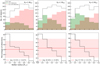 |
Fig. 2 Results from the injecting artificial transit test. Top row: result for injected planets with radius Rp = 1.0 RJup (left), for planets with radius Rp = 1.5 RJup (middle), and for planets with radius Rp = 2.0 RJup (right). The green shaded areas shows the correctly detected artificial transits for different stellar radii, while the red shaded areas show the non-detections. The black line shows the total number of injected planets for the different stellar radii. Bottom row: percentages of correctly detected artificial transits for stellar radii in the range 2. R⊙ ≤ R ≤ 5 R⊙. The red line indicates the average percentage and the red shaded area indicates the 1σ errors. |
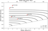 |
Fig. 3 Expected orbital evolution of Jupiter-mass planets orbiting a red giant of mass 1.5 M⊙, on orbits with initial semi-major axis within the range 0.02-0.10 AU, following Kunitomo et al. (2011). The HJs in our sample are indicated; Kepler-91 is included for comparison. |
5.3 Future searches
The occurrence rate estimate presented in this work is based on only a few objects and may be prone to biases due to the detection probability being a strong function of stellar apparent magnitude and stellar radius. Since TESS continues to observe, the available data to search for HJs around red giant stars will only increase and mitigate this issue. It may also help to conduct a more sensitive study using difference imaging analysis (Oelkers & Stassun 2018; Montalto et al. 2020) or a principle component analysis (see, e.g., the eleanor Feinstein et al. 2019; or the Giants Saunders et al. 2022 pipelines) to the light curves obtained from the FFIs. These pipelines could yield cleaner light curves, an increase in detection probability, and a more precise estimate for the occurrence rate. For example, our method has missed one possible candidate, TOI-4551.013, due to transit-like signals in the light curve, which are likely related to the momentum dumps occurring during the observations. Using one of these two pipelines could lead to the inclusion of such candidates.
In the future, the ESA PLATO mission (Rauer 2017) may result in high-precision light curves for a large sample of red giant stars from which HJs can be discovered and their occurrence rate further constrained.
Acknowledgements
This work has made use of data from the European Space Agency (ESA) mission Gaia (https://www.cosmos.esa.int/gaia), processed by the Gaia Data Processing and Analysis Consortium (DPAC, https://www.cosmos.esa.int/web/gaia/dpac/consortium). Funding for the DPAC has been provided by national institutions, in particular the institutionsparticipating in the Gaia Multilateral Agreement. This paper includes data collected by the TESS mission. Funding for the TESS mission is provided by the NASA’s Science Mission Directorate. This work has used the following additional software packages that have not been referred to in the main text: Numpy, Matpotlib, IPython and Pandas (Harris et al. 2020; Hunter 2007; Pérez & Granger 2007; pandas development team 2020).
Appendix A Gaussian processed light curves
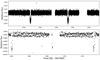 |
Fig. A1 Gaussian processed light curve of HD 1397. |
Appendix B Fitted light curves
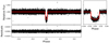 |
Fig. B1 Best fit to the light curve of HD 1397. The top left panel shows the phase-folded light curve with the best fit as the red line, while the bottom panel shows the residuals. The top right panel shows a zoomed-in version of the phase-folded transit. |
Median values and 1σ confidence limits of the fitted parameters for the star HD 1397.
References
- Astropy Collaboration (Robitaille, T. P., et al.) 2013, A&A, 558, A33 [NASA ADS] [CrossRef] [EDP Sciences] [Google Scholar]
- Astropy Collaboration (Price-Whelan, A. M., et al.) 2018, AJ, 156, 123 [Google Scholar]
- Borucki, W. J., Koch, D. G., Basri, G., et al. 2011, ApJ, 736, 19 [Google Scholar]
- Brahm, R., Espinoza, N., Jordán, A., et al. 2019, AJ, 158, 45 [Google Scholar]
- Ciceri, S., Lillo-Box, J., Southworth, J., et al. 2015, A&A, 573, L5 [NASA ADS] [CrossRef] [EDP Sciences] [Google Scholar]
- Dawson, R. I., & Johnson, J. A. 2018, ARA&A, 56, 175 [Google Scholar]
- Espinoza, N., Kossakowski, D., & Brahm, R. 2019, MNRAS, 490, 2262 [Google Scholar]
- Feinstein, A. D., Montet, B. T., Foreman-Mackey, D., et al. 2019, PASP, 131, 094502 [Google Scholar]
- Foreman-Mackey, D., Hogg, D. W., Lang, D., & Goodman, J. 2013, PASP, 125, 306 [Google Scholar]
- Fressin, F., Torres, G., Charbonneau, D., et al. 2013, ApJ, 766, 81 [NASA ADS] [CrossRef] [Google Scholar]
- Gaia Collaboration (Prusti, T., et al.) 2016, A&A, 595, A1 [NASA ADS] [CrossRef] [EDP Sciences] [Google Scholar]
- Gaia Collaboration (Babusiaux, C., et al.) 2018, A&A, 616, A10 [NASA ADS] [CrossRef] [EDP Sciences] [Google Scholar]
- Grunblatt, S. K., Huber, D., Gaidos, E., et al. 2019, AJ, 158, 227 [Google Scholar]
- Grunblatt, S. K., Saunders, N., Sun, M., et al. 2022, AJ, 163, 120 [NASA ADS] [CrossRef] [Google Scholar]
- Harris, C. R., Millman, K. J., van der Walt, S. J., et al. 2020, Nature, 585, 357 [NASA ADS] [CrossRef] [Google Scholar]
- Huber, D., Carter, J. A., Barbieri, M., et al. 2013, Science, 342, 331 [Google Scholar]
- Huber, D., Chaplin, W. J., Chontos, A., et al. 2019, AJ, 157, 245 [Google Scholar]
- Hunter, J. D. 2007, Comput. Sci. Eng., 9, 90 [NASA ADS] [CrossRef] [Google Scholar]
- Jenkins, J. M., Twicken, J. D., McCauliff, S., et al. 2016, SPIE, 9913, 1232 [Google Scholar]
- Kippenhahn, R., Weigert, A., & Weiss, A. 2012, Stellar Structure and Evolution (Berlin: Springer) [Google Scholar]
- Kipping, D. M. 2014, MNRAS, 444, 2263 [NASA ADS] [CrossRef] [Google Scholar]
- Kunitomo, M., Ikoma, M., Sato, B., Katsuta, Y., & Ida, S. 2011, ApJ, 737, 66 [Google Scholar]
- Lillo-Box, J., Barrado, D., Moya, A., et al. 2014, A&A, 562, A109 [NASA ADS] [CrossRef] [EDP Sciences] [Google Scholar]
- Lillo-Box, J., Barrado, D., & Correia, A. C. M. 2016, A&A, 589, A124 [NASA ADS] [CrossRef] [EDP Sciences] [Google Scholar]
- Lund, M. N., Handberg, R., Davies, G. R., Chaplin, W. J., & Jones, C. D. 2015, ApJ, 806, 30 [NASA ADS] [CrossRef] [Google Scholar]
- Masuda, K., & Winn, J. N. 2017, AJ, 153, 187 [NASA ADS] [CrossRef] [Google Scholar]
- Montalto, M., Borsato, L., Granata, V., et al. 2020, MNRAS, 498, 1726 [NASA ADS] [CrossRef] [Google Scholar]
- Nielsen, L. D., Bouchy, F., Turner, O., et al. 2019, A&A, 623, A100 [NASA ADS] [CrossRef] [EDP Sciences] [Google Scholar]
- Oelkers, R. J., & Stassun, K. G. 2018, AJ, 156, 132 [NASA ADS] [CrossRef] [Google Scholar]
- Pandas development team, 2020, https://github.com/pandas-dev/pandas/tree/main/pandas [Google Scholar]
- Parviainen, H. 2015, MNRAS, 450, 3233 [Google Scholar]
- Paxton, B., Bildsten, L., Dotter, A., et al. 2011, ApJS, 192, 3 [Google Scholar]
- Paxton, B., Cantiello, M., Arras, P., et al. 2013, ApJS, 208, 4 [Google Scholar]
- Paxton, B., Marchant, P., Schwab, J., et al. 2015, ApJS, 220, 15 [Google Scholar]
- Paxton, B., Schwab, J., Bauer, E. B., et al. 2018, ApJS, 234, 34 [NASA ADS] [CrossRef] [Google Scholar]
- Paxton, B., Smolec, R., Schwab, J., et al. 2019, ApJS, 243, 10 [Google Scholar]
- Pepper, J., Rodriguez, J. E., Collins, K. A., et al. 2017, AJ, 153, 215 [NASA ADS] [CrossRef] [Google Scholar]
- Pérez, F., & Granger, B. E. 2007, Comput. Sci. Eng., 9, 21 [Google Scholar]
- Petigura, E. A., Marcy, G. W., Winn, J. N., et al. 2018, AJ, 155, 89 [Google Scholar]
- Quinn, S. N., White, T. R., Latham, D. W., et al. 2015, ApJ, 803, 49 [NASA ADS] [CrossRef] [Google Scholar]
- Rauer, H. 2017, in EGU General Assembly Conference Abstracts, EGU General Assembly Conference Abstracts, 4829 [Google Scholar]
- Reimers, D. 1975, Mem. Soc. R. Sci. Liege, 8, 369 [NASA ADS] [Google Scholar]
- Saunders, N., Grunblatt, S., & Huber, D. 2022, BAAS, 54, 102.230 [Google Scholar]
- Stassun, K. G., Oelkers, R. J., Paegert, M., et al. 2019, AJ, 158, 138 [Google Scholar]
- Van Eylen, V., Albrecht, S., Gandolfi, D., et al. 2016, AJ, 152, 143 [NASA ADS] [CrossRef] [Google Scholar]
- Vanderburg, A., & Johnson, J. A. 2014, PASP, 126, 948 [Google Scholar]
- Vanderburg, A., Latham, D. W., Buchhave, L. A., et al. 2016, ApJS, 222, 14 [Google Scholar]
- Zhou, G., Huang, C. X., Bakos, G. Á., et al. 2019, AJ, 158, 141 [Google Scholar]
Tesseract: https://github.com/astrofelipe/tesseract
The observed hot Jupiters were acquired from Exoplanet.eu (http://exoplanet.eu/, on July 18, 2022) using the query: RADIUS:RJUP >=1 AND RADIUS:RJUP <= 2 AND PERIOD:DAY <= 15.
ExoFOP-page of TOI-4551.01: https://exofop.ipac.caltech.edu/tess/target.php?id=204650483
All Tables
Stellar masses, stellar radii, planetary radii, planetary masses, and semi-major axes used in the calculation for the geometric probability.
Median values and 1σ confidence limits of the fitted parameters for the star HD 1397.
All Figures
|
Fig. 1 Colour-magnitude diagram of stars that have survived the imposed selection criteria. The black box represents the boundaries of the region enclosing the RGB. The colour (GBP − GRP) of the stars can be found on the x-axis, while the y-axis denotes the absolute magnitudes. The logarithmic colour map indicates the number of stars in each two-dimensional bin. Stars removed by the selection criteria are shown in grey. |
| In the text | |
|
Fig. 2 Results from the injecting artificial transit test. Top row: result for injected planets with radius Rp = 1.0 RJup (left), for planets with radius Rp = 1.5 RJup (middle), and for planets with radius Rp = 2.0 RJup (right). The green shaded areas shows the correctly detected artificial transits for different stellar radii, while the red shaded areas show the non-detections. The black line shows the total number of injected planets for the different stellar radii. Bottom row: percentages of correctly detected artificial transits for stellar radii in the range 2. R⊙ ≤ R ≤ 5 R⊙. The red line indicates the average percentage and the red shaded area indicates the 1σ errors. |
| In the text | |
|
Fig. 3 Expected orbital evolution of Jupiter-mass planets orbiting a red giant of mass 1.5 M⊙, on orbits with initial semi-major axis within the range 0.02-0.10 AU, following Kunitomo et al. (2011). The HJs in our sample are indicated; Kepler-91 is included for comparison. |
| In the text | |
|
Fig. A1 Gaussian processed light curve of HD 1397. |
| In the text | |
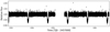 |
Fig. A2 Same as Fig. A1, but for the star KELT-11. |
| In the text | |
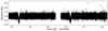 |
Fig. A3 Same as Fig. A1, but for the star HD 221416. |
| In the text | |
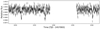 |
Fig. A4 Same as Fig. A1, but for the star TYC-5456-76-1. |
| In the text | |
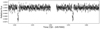 |
Fig. A5 Same as Fig. A1, but for the star CD-25 2180. |
| In the text | |
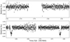 |
Fig. A6 Same as Fig. A1, but for the star TYC-4004-1387-1. |
| In the text | |
|
Fig. B1 Best fit to the light curve of HD 1397. The top left panel shows the phase-folded light curve with the best fit as the red line, while the bottom panel shows the residuals. The top right panel shows a zoomed-in version of the phase-folded transit. |
| In the text | |
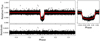 |
Fig. B2 Same as Fig. B1, but for the star KELT-11. |
| In the text | |
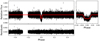 |
Fig. B3 Same as Fig. B1, but for the star HD 221416. |
| In the text | |
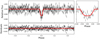 |
Fig. B4 Same as Fig. B1, but for the star TYC-5456-1. |
| In the text | |
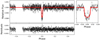 |
Fig. B5 As figure B1, but for the star CD-25 2180. |
| In the text | |
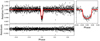 |
Fig. B6 Same as Fig. B1, but for the star TYC-4004-1387-1. |
| In the text | |
Current usage metrics show cumulative count of Article Views (full-text article views including HTML views, PDF and ePub downloads, according to the available data) and Abstracts Views on Vision4Press platform.
Data correspond to usage on the plateform after 2015. The current usage metrics is available 48-96 hours after online publication and is updated daily on week days.
Initial download of the metrics may take a while.