| Issue |
A&A
Volume 669, January 2023
|
|
|---|---|---|
| Article Number | A78 | |
| Number of page(s) | 10 | |
| Section | Astronomical instrumentation | |
| DOI | https://doi.org/10.1051/0004-6361/202244640 | |
| Published online | 13 January 2023 | |
Effects of solar evolution on finite acquisition time of Fabry–Perot interferometers in high resolution solar physics
Leibniz-Institut für Sonnenphysik (KIS),
Schöneckstr. 6,
79104
Freiburg, Germany
e-mail: This email address is being protected from spambots. You need JavaScript enabled to view it.
Received:
30
July
2022
Accepted:
24
October
2022
Abstract
Context. The Visible Tunable Filter (VTF) imaging spectropolarimeter will be operated at the Daniel K. Inouye Solar Telescope (DKIST) in Hawaii. Due to its capability in resolving dynamic fine structure of smaller than 0.05 arcsec, the finite acquisition time of typically 11 s affects the measurement process and potentially causes errors in deduced physical parameters.
Aims. We estimate these errors and investigate ways of minimising them.
Methods. We mimicked the solar surface using a magnetohydrodynamic simulation with a spatially averaged vertical field strength of 200 G. We simulated the measurement process scanning through successive wavelength points with a temporal cadence of 1 s. We synthesised Fe 1617.3 nm for corresponding snapshots. In addition to the classical composition of the line profile, we introduce a novel method where the intensity in each wavelength point is normalised using the simultaneous continuum intensity, and then multiplied by the temporal mean of the continuum intensity. Milne-Eddington inversions were used to infer the line-of-sight velocity, vlos, and the vertical (longitudinal) component of the magnetic field, Blos.
Results. We quantify systematic errors, defining the temporal average of the simulation during the measurement as the truth. We find that with the classical composition of the line profiles, errors exceed the sensitivity for vlos, and in filigree regions also for Blos. The novel method that includes normalisation reduces the measurement errors in all cases. Spatial binning without reducing the acquisition time decreases the measurement error slightly.
Conclusions. The evolutionary timescale in inter-granular lanes, in particular in areas with magnetic features (filigree), is shorter than the timescale within granules. Hence, depending on the science objective, fewer accumulations could be used for strong magnetic field in inter-granular lanes and more accumulations could be used for the weak granular magnetic fields. As a key result of this investigation, we suggest including the novel method of normalisation in corresponding data pipelines.
Key words: Sun: magnetic fields / instrumentation: polarimeters / instrumentation: high angular resolution / Sun: photosphere
© The Authors 2023
 Open Access article, published by EDP Sciences, under the terms of the Creative Commons Attribution License (https://creativecommons.org/licenses/by/4.0), which permits unrestricted use, distribution, and reproduction in any medium, provided the original work is properly cited.
This article is published in open access under the Subscribe-to-Open model. This email address is being protected from spambots. You need JavaScript enabled to view it. to support open access publication.
1 Introduction
The solar photosphere and chromosphere are highly dynamic and exhibit a wealth of magnetic structures and phenomena. The underlying processes operate on small spatial and temporal scales and are a consequence of fundamental interactions between plasma, magnetic fields, and radiation. These interactions leave spectropolarimetric imprints in absorption and emission lines, which form in the photosphere and chromosphere, that can be measured with sophisticated instrumentation. Classically, there are two types of instruments: slit-scanning spectrographs and narrow-band imagers scanning in wavelength through a spectral line. Both types can be equipped with polarimetric modulators. While grating spectrographs have the advantage of spectral integrity, high spectral resolution, and large spectral coverage, Fabry–Perot interferometer (FPI) narrow-band imagers have the advantage of image integrity, large fields of view, and short cadences. New technical developments aim to combine spectral and image integrity with short cadences in integral field units. Currently, two concepts look very promising: image slicers and micro-lense arrays (see e.g. Jurčák et al. 2019; Kaithakkal et al. 2020; Dominguez-Tagle et al. 2022).
Here, we investigate the spectral integrity of an FPI-based narrow-band imager that may suffer from scanning in wavelength through a spectral line, resulting in a finite acquisition time, during which the solar scene may change (as already noted in Schubert et al. 2017). We use the Visible Tunable Filter (VTF, Schmidt et al. 2014) which is planned to be installed in 2023 at the Daniel K. Inouye Solar Telescope (DKIST, Rimmele et al. 2020). VTF is an imaging spectropolarimeter for the wavelength range between 520 and 860 nm. It is based on two FPIs1 that scan the narrow-band images in wavelength, which means that the spectral points of a solar line are not acquired simultaneously, but during a finite acquisition time. In general, the integration time at each wavelength step is determined by the desired signal-to-noise ratio (S/N, i.e. polarimetric sensitivity). A default measurement at full spatial resolution of the photospheric magnetic field with VTF in Fe 1617.3 nm takes 11 s to reach the desired polarimetric accuracy at 11 wavelength points (see Sect. 2). VTF is designed to operate at the diffraction limit of DKIST, which has an aperture of 4 m (i.e. at 520 nm scales of 20 km are resolved on the solar surface). On such small scales, dynamical processes in the solar photosphere potentially lead to spurious signals that spoil the measurement.
Short timescales observed with GREGOR
To demonstrate these short timescales in the solar photosphere, in Fig. 1 we present images from GREGOR (Schmidt et al. 2012; Berkefeld et al. 2012) taken with HiFI (Denker et al. 2018) close to the disc centre on June 30, 2019, in the G band. The images are Speckle-reconstructed with KISIP (Wöger et al. 2008) by selecting the 100 best out of 500 images.
The upper large panel of Fig. 1 shows the observed active filigree region at 08:22:21 UT. Four consecutive snapshots with a time lapse of about 11.5 s are displayed in the four small panels for the region enclosed by the white box in the large panel. The small panels have a side width of 2 arcsec and contain 672 pixel with a width of 0.03 arcsec. The solar scene within the 35 s is clearly not static, and changes on scales of 0.1 arcsec are already visible in the consecutive images, where the temporal spacing is 11s. The evolution is tiny, but clearly visible on small spatial scales.
In this contribution, we investigate the effects of spurious signals that are expected from temporal evolution during the measurement process. The evolution is mimicked by a realistic magneto-hydrodynamic simulation of a plage region. The VTF measurement process is described in Sect. 2. The method we applied to mimic the measurement process and how to describe the measurement error is explained in Sect. 3. Our results are presented and discussed in Sect. 4. Section 5 presents our conclusion and an important suggestion concerning the data pipeline of Fabry–Perot-based spectropolarimeters.
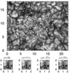 |
Fig. 1 Speckle-reconstructed images of a filigree region close to disc centre observed with HiFi at GREGOR on June 30, 2019, in G band at 430 nm. The upper large panel shows a large FOV at 08:22:21 UT. The four small lower panels show four subsequent snapshots t = 0, 11, 23, and 35 s of a smaller FOV (white box in upper panel). The tick marks indicate units in arcsec. |
2 VTF measurement process
The VTF measurement process is described in Schmidt et al. (2014) and summarised here as follows. The cameras of VTF have a pixel size of 12 µm, which corresponds to 0.014 arcsec and 10 km on the sun. This corresponds to a diffraction-limited spatial resolution of 0.028 arcsec at a wavelength of 520 nm.
To reach its spectral resolution of λ/Δλ = 100000, the wavelength spacing amounts to 3 pm at a wavelength of 600 nm. For our study we use Fe 1617.3 nm (g = 2.5), which has very similar properties to Fe 1630.2 nm. The VTF cameras are operated with a frame cycle time of 40 ms, of which 25 ms are used as exposure time. Simultaneously with each narrow-band image, a broad-band image is recorded in a separate channel of the instrument.
The VTF can be operated in spectroscopic and spectropolarimetric mode. For both modes the number of scanning steps, number of accumulations, and the binning size can be adjusted. The VTF Instrument Performance Calculator (IPC, Version 3.4)2 was developed to tune these free parameters and to estimate the resulting S/N as well as the time of the measurement. We note that the IPC calculates the S/N for Stokes I, and does not take into account polarimetric efficiencies. A default spectroscopic measurement with one accumulation at full spatial resolution with a S/N above 200 takes less than one second (=0.88 s) to measure, for example Fe 1617.3 nm with 11 wavelength scan steps (each scan step to tune the FPIs takes one camera cycle time of 40 ms). In the photosphere, changes in physical parameters on a timescale of one second are not expected within resolution elements as large as 20 km.
Spectropolarimetric measurements take more time, on the one hand because four modulation states need to be measured instead of one, and on the other hand because the polarimetric signal in the spectral line is weak and requires a large number of photons. To minimise seeing-induced cross-talk, in addition to doing dual-beam polarimetry, the four modulation states are acquired consecutively with four single exposures. To increase the number of photons and reduce the photon noise, consecutive accumulations can be chosen at each wavelength position. With six accumulations, a 1σ noise level of 1/577 = 0.0017 is reached (with continuum intensity being normalised to 1). To detect a signal it should have a minimum amplitude of 3σ, which corresponds to about 0.005. This limits the minimum magnetic field strength which can be detected. In our case computing synthetic line profiles for Fe 1617.3 nm of a quiet-Sun model and a spectral resolution of 100 000, we find that a Stokes V amplitude of 0.005 is produced by a constant vertical field of ~20 G at disc centre (cf., Schubert 2016; Schubert et al. 2017). We note that a horizontal homogeneous field needs 175 G to produce a Q-signal of 0.005. With a horizontal field strength of 100 G, the Q-amplitude amounts to 0.0017 (see also Borrero & Kobel 2012, 2013).
Schmidt et al. (2016) estimate the Doppler shift sensitivity to approximately 80 m s−1, taking into account photon noise and stray light. We note that non-parallelism of the FPI plates was not considered as a source of error in this estimate.
With six accumulations, 6 × 4 = 24 single frames are recorded at each wavelength step; 11 spectral points are measured in 11 s (i.e. 1 s per spectral point). This means that a single spectropolarimetric VTF measurement with six accumulation takes 11 s in total. The task of this contribution is to investigate, based on realistic numerical simulations, whether dynamic changes are expected in the photosphere within 11 s, and if yes, how much these changes affect the measurement. We note that many science cases require a noise level lower than 0.0017. With 12 accumulations, which take 21.6 s, VTF reaches a 1σ noise level of 0.0012; instead, 18 accumulations and 31 s are needed to reach a noise level of 10−3. Measurements with longer scanning times are more affected by the dynamic evolution in the photosphere. However, in this contribution we assume that the measurement process takes 11 seconds for 11 scan steps (i.e. we imitate the case of six accumulations).
3 Methods
To mimic the measurement process of VTF, we took consecutive snapshots of a realistic magnetohydrodynamic simulation of a solar plage region (Sect. 3.1), synthesised Stokes profiles and adapted them to the VTF spectral resolution and acquisition procedure (Sect. 3.2). In Sect. 3.3, we introduce an alternative way to construct the line profiles, normalising each wavelength point to the local continuum intensity. As a result, we produced different sets of Stokes profiles from the 11 time steps of the simulation. In Sect. 3.4, we describe how these different sets of profiles are inverted to retrieve the physical parameters of the line-of-sight velocity and the vertical component of the magnetic field strength.
To quantify the error of the measurement process, we need to define a reference or true map. As true maps, we use the maps that result from the inversion of profiles that are synthesised from time-averaged simulation boxes (over all 11 snapshots), which means that these profiles are not affected by the finite acquisition time, and therefore serve as reference. Finally, all the different sets of maps are compared in Sect. 4. By comparing the physical parameters between the inverted maps from constructed profiles and the reference maps, we can estimate the error that is introduced by the finite acquisition time.
3.1 Solar plage simulation with MURAM
As a typical target for VTF observations we take a plage region with a spatially averaged vertical magnetic strength of 200 G. This simulation was performed with MURAM by Matthias Rempel (private communications, and see Rempel 2014). With a grid cell size of 8×8×8 km3, the simulation reaches the spatial resolution of VTF mounted at DKIST. The simulation box has 768×768×384 cells. The box reaches from the upper photosphere into the solar interior. The upper end of the box lies 704 km above the average τ = 1 level. As the lateral box sides have periodic boundary conditions, the magnetic flux through each depth layer is the same and is constant in time.
The internal numerical time step of the simulation is around 0.1 s. We limit our analysis to snapshots with a temporal cadence of 1 s (i.e. ten numerical time steps). Changes within ten time steps can be considered small for our purpose, but they contribute to an increase in the measurement errors. For this work we assume that it is sufficient to have a snapshot sequence of 1 s. This is the same cadence that VTF needs for each wavelength step when using six accumulations (S/N = 577).
In Fig. 2a, we display a vertical cut of the absolute magnetic field strength of the computational box. It displays a vertical strong flux concentration in the middle of the box at x = 3 Mm. There the local field strength exceeds 3 kG. For the horizontal layer at which the spatially averaged temperature is 5560 K, we show the vertical components of the velocity and the vertical magnetic field strength in Figs. 2b and c. This horizontal layer roughly corresponds to the formation height of Fe I 630.25 nm such that these maps can be compared with the maps that we retrieve after line synthesis, convolution with the VTF spectral resolution, resampling, and Milne-Eddington inversion.
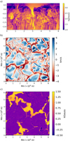 |
Fig. 2 MURAM simulation snapshot. (a) Vertical cut through numerical box showing the modulus of the magnetic field strength in logarithmic scale, clipped between 10 and 2500 G, with the colour bar in logarithmic scale. (b) Horizontal cut at mean temperature of 5560 K of vertical velocity in km s−1 with positive values pointing upwards (being blue-shifted to observer). (c) Same as panel b, but for the vertical component of the magnetic field strength in kG. |
3.2 Synthetic line profiles with FIRTEZ adapted to VTF
From a number of suitable photospheric absorption lines we chose to analyse the Fe 1617.3 nm3. VTF will use Fe 1630.25 nm for the first observations as long as only one FPI is available, but Fe I 617.3 nm will be available as soon as the second FPI is in place.
To synthesise Stokes I, Q, U, and V of Fe I 617.3 nm along vertical lines of sight in the MURAM box, we used FIRTEZ-dz (Pastor Yabar et al. 2019). FIRTEZ was chosen because it operates on the geometrical scale, which is intrinsic to the simulation box. As the conversion into optical depth along the line of sight is not needed, the computation time for the line synthesis is very short. We calculated the set of Stokes profiles for each horizontal pixel yielding maps with 768 by 768 pixel.
For the line synthesis the spectral resolution is assumed to be infinity, and is only limited by the spectral sampling. We used a spectral sampling of 0.4 pm, and computed the range from − 40 pm to +40 pm.
Spectral convolution and spectral sampling
The spectral resolution of VTF follows from the properties of the first FPI. The spectral transmission profile (see e.g. Sect. 3.4.4 in Stix 2002) can be computed for small angles of incidence from its reflectance, R = 0.95, and its cavity separation, d = 0.55 mm (Kentischer et al. 2012; Schmidt et al. 2014; Sigwarth 2017). A prefilter is assumed to suppress the side peaks and to transmit only the central peak. The transmission profile of the central peak corresponds to a spectral resolution of 100 000 and has a full width at half maximum of 5.7 pm. All FIRTEZ profiles are convolved with this transmission profile and resampled to the VTF spectral step width of Δλ = 3.15 pm. A set of sample profiles are depicted in Fig. 3. The synthetic lines of Stokes I, Q, U, and V of a sample pixel are drawn in red. The blue lines display the same profiles after accounting for the spectral resolution of VTF, and the blue crosses show the spectral sampling of VTF. To sketch the shape of the tuneable VTF transmission profile, it is plotted as a green line in the Stokes U plot. Thus, in the end we have Stokes profiles (at the spectral resolution and sampling of VTF) for a set of 11 snapshots, which have a temporal cadence of 1s.
Temporal sampling
To mimic the VTF line scan, we composed the Stokes profiles with one wavelength step per consecutive snapshot; in other words, we produced a set of profiles with 11 wavelength points (t = 0, 1, …, 10 s). We do this in two modes: straight and rabbit. In the straight mode the wavelength step increases monotonically by one: λi+1 = λi + Δλ. In the rabbit mode we jump from the blue wing to the red wing, successively approaching the line core: λi+1 = λi + 2 * (λic − λi) and λi+2 = λi + Δλ, with λic being the wavelength step closest to the spatially averaged line core. The idea of the rabbit mode is to sample both line wings as close in time as possible. Here, the Doppler shift error from the finite acquisition time is expected to be minimised.
Seeing and solar evolution
The rabbit mode was devised for VTF to also minimise the effects of seeing. The seeing is partially corrected by the adaptive optics system. The resulting degree of image correction varies on scales of seconds and shorter. With the rabbit mode the goal is to record the two line wings with similar seeing. However, the effects of seeing are not analysed in this work. We ignore seeing effects, and only consider the effects of solar evolution during the line scan.
Reference profile and temporal changes
In order quantify the systematic measurement errors, we need to define a reference. We used profiles from temporally averaged snapshots for each pixel as the reference, which means that we averaged all 11 snapshots and performed the line synthesis on the averaged box. Alternatively, it is possible to average the synthesised profiles from the 11 snapshots and do the inversion on the time-averaged profiles. We checked that both approaches lead to identical results within the noise, which is on the same scale as the difference between two consecutive snapshot maps.
In Fig. 4, we illustrate the temporal change of the profiles. We select a sample pixel and plot the Stokes profiles retrieved from the first snapshot 1 (blue line), from the last snapshot 11 (red line), and from the temporally averaged profiles from all 11 snapshots (black line). In the upper left panel, it can be seen that the intensity of the left-most wavelength point drops from approximately 1.28 to 1.02 (i.e. by more than 25% during the measurement process across 11 wavelength points).
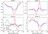 |
Fig. 3 Stokes I, Q, U, and V profiles (from upper left to lower right). The red line denotes synthesised profiles with intrinsic sampling of 0.4 pm. The green line in the lower left panel sketches the shape of the VTF transmission curve. Blue crosses and lines mimic 11 VTF measurement points as a result of convolving the synthetic profiles with the VTF transmission curve. |
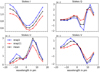 |
Fig. 4 Example pixel of the Stokes profiles for t = 0 s (blue) and t = 10 s (red) is plotted. The black curve shows the profile from a temporal average of all 11 snapshots. |
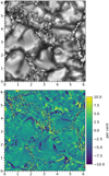 |
Fig. 5 Change of continuum intensity during line scan. Upper panel: continuum image with intensities between 0.6 and 1.45 for the first snapshot. The average intensity is normalised to one. Lower panel: difference between the continuum images of snapshot 1 and snapshot 11. The difference map is clipped at differences of ±10%. |
3.3 Profile composition with normalisation
Viewing animations of the snapshots, it becomes apparent that magnetic concentrations, which are visible as bright points in the inter-granular lanes, are shuffled around by the granular flow field. As a consequence, the continuum intensity of an inter-granular pixel can change significantly during the wavelength scan. This is demonstrated in Fig. 5, where we display the normalised continuum intensity of the first snapshot and the difference map between the first (snapshot 1) and last (snapshot 11) snapshot. The difference map is clipped at absolute differences of 0.1. We compute that in 13% of all pixels the intensity difference is larger than 0.05, and in 4% of all pixels the difference is larger than 0.1. The standard deviation amounts to 0.034. In comparison, the standard deviation of intensity differences between the first and second snapshot amounts to 0.006.
If the continuum intensity, for example, decreases continuously during a straight wavelength scan, an analysis of the corresponding composed Stokes I profile would yield different intensity levels of the blue and red continua. This would be interpreted as an additional line absorption in the red wing (i.e. as an enhanced red-shift). This example suggests that it might be an advantage to normalise the line absorption to the continuum. Since we have the full simulated profiles at each time step (= wavelength step), it is possible to do this. Obviously, this is not straightforward for the VTF measurement. However, as VTF is operated with a simultaneous broad-band channel, this normalisation could be performed using the broad-band intensity as it varies during the line scan at a given spatial pixel.
In Fig. 6, we illustrate how the straight profile is normalised, and compare the different Stokes I profile types for the same spatial pixel as in Fig. 4. The black line displays the time-averaged profile. The red line displays the straight VTF measurement mode. The rabbit mode behaves similarly to the straight profiles and is not displayed. The green line denotes the continuum intensity variation during the measurement process. From these continuum points, the temporal mean is calculated. This mean value, 〈I(conti)〉i=1,…11, is used to normalise each wavelength point of the straight profile (red line):
 (1)
(1)
This normalised profile is drawn as blue line in Fig. 6, which shows that the normalised straight profile becomes very similar to the time-averaged profile. Therefore, we expect the normalised profiles to lead to physical parameters that are closer to the reference (time-averaged) parameters. For pixels in which the continuum intensity is constant in time, the straight, normalised, and time-averaged profiles are identical.
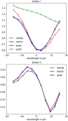 |
Fig. 6 Comparison of Stokes I and V profiles in upper and lower panel, respectively: Straight composed (red) simulating the VTF measurement, straight normalised (blue), and time-average. The green line in the upper panel denotes the continuum intensity at each wavelength (=time) step. |
3.4 Milne-Eddington inversion with VFISV
To compare the differently composed Stokes profiles, we performed Milne-Eddington inversions and compared inverted maps of the line-of-sight velocities, vlos, and of the vertical (line-of-sight) component of the magnetic field strength, Blos, for the different profile types. The Milne-Eddington approximation assumes that vlos, B, and Blos are constant along the line of sight across the solar photosphere. An inspection of the numerical simulation (see e.g. the vertical cut of Blos in Fig. 3.1) shows that this is clearly not the case, and these quantities change significantly along the line of sight. However, in order not to introduce additional error sources due to sophisticated inversions, we limit our analysis to Milne-Eddington inversions.
As inversion code, we used the “Very Fast Inversion of the Stokes Vector” (VFISV, Borrero et al. 2011). This code was originally devised to invert data from the Helioseismic and Magnetic Imager (HMI) on board the Solar Dynamic Observatory (SDO), and was later adapted to data acquired with slit spectrographs4 as for GRIS installed at GREGOR (Collados et al. 2012), and to data acquired with Fabry–Perot systems5. In the Fabry–Perot version, the VTF transmission file can be selected in such a way that it is taken into account in the inversion process. We note that we use the identical transmission profile in the convolution with the synthetic profiles in Sect. 3.2. As free parameters we use η0, field inclination γ, field azimuth ϕ, damping a, Doppler width ∆λD, field strength B, line-of-sight velocity vlos, source function continuum, and the source function gradient. The magnetic filling factor is put to unity and is not used as free parameter.
4 Results and discussions
4.1 Inverted maps for reference (time-averaged) profiles
Inverted maps for vlos and Blos = B · cos(γ) of the reference (time-averaged) profiles are displayed in Fig. 7. These maps correspond to the average along the line of sight, but for consistency, they can be compared to the horizontal geometrical cuts at the mean temperature of 5560 K in Figs. 2 b and c. In both figures, we use the same colour-coding and clipping values. They are obtained after line synthesis with FIRTEZ on the time-averaged numerical box, convolution with the instrument transmission profile (Sect. 3.2), and VFISV inversion (Sect. 3.4).
These maps reflect the ideal theoretical expectation of what VTF mounted at DKIST will measure in a plage region with an average vertical magnetic field strength of 200 G. It is therefore of interest to plot the histogram distribution for vlos and Blos in Fig. 8. Both distributions are non-symmetric. The up-flow velocities do not reach values as high as the down-flow velocities, but occupy a larger area for small absolute values. Opposite polarity in the magnetic field is present and reaches values of up to – 400 G. The distribution of the positive vertical component of the magnetic field peaks at approximately 1300 G and Blos reaches values of up to 2.4 kG.
4.2 Average of the vertical magnetic field strength
The horizontal average vertical magnetic field strength (magnetic flux through a horizontal cut) in the simulation box is constant at all depth layers and at all times due to the periodic boundary conditions on the sides of the box. It was chosen to be 200 G. This number can be compared with maps of Blos for the various types of profiles. Averaging the Blos across the inverted maps we obtain 〈Blos〉 = 208 G for the reference profiles, 203 G for the straight VTF profiles, 206 G for the rabbit VTF profiles, 208 G for the straight normalised VTF profiles, and 208 G for profiles of each snapshot.
The difference of 8 G between the numerical box value and the reference map is ascribed to the different geometrical formation heights. We surmise that strong field concentrations are associated with smaller densities, due to magnetic evacuation (magnetic pressure). Hence, in areas of magnetic field concentration, the opacity is reduced and the line forms in deeper geometrical layers in which the field strength is stronger. This effect could explain that the average value 〈Blos〉 in the inverted reference map is larger by 8 G than in the numerical box at constant geometrical height. In any case, the difference is small and not significant for our study.
More interesting for our study is the finding that normalised straight VTF profiles yield the same 〈Blos〉 as the reference profiles, while the straight VTF profiles differ by 5 G. This difference is small, but confirms the expectation (Fig. 6 in Sect. 3.3) that the normalised VTF profiles are closer to the reference (time averaged) profiles.
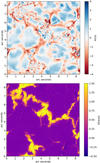 |
Fig. 7 Maps for line-of-sight velocity, vlos (upper panel), and vertical component of the magnetic field strength, Blos (lower panel), inverted with VFISV from reference (time-averaged) Stokes profiles. As these maps are simulated observables, arcsec are used instead of km for the spatial dimension. |
4.3 Oscillation of the numerical box
Similarly to Sun, the MURAM box exhibits five-minute oscillations that are visible in maps of vlos. Therefore the average line-of-sight velocity is not constant. The particular snapshots that we analyse change from a mean velocity of 41 m s−1 in the first snapshot by approximately 2 m s−1 to 18 m s−1 in the eleventh snapshot. Hence, the spatially averaged vlos changes by 21 m s−1 during the analysed VTF measurement process.
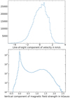 |
Fig. 8 Histograms for maps of line-of-sight velocity with a bin size of 115 m s−1 (upper panel), and vertical component of the magnetic field strength with a bin size of 30 G (lower panel) for the inverted maps of the reference (time-averaged) profiles. |
4.4 Difference maps for maps of vlos and Blos
As explained in Sect. 1, the purpose of this study is to quantify the measurement error due to a finite measurement time of 11 s. To determine the error we compare simulated VTF maps to the reference (time-averaged) maps by computing difference maps. In the upper two panels of Figs. 9 and 10, we display the difference maps from the inversion of straight VTF profiles and the straight normalised VTF profiles with the reference maps. For vlos, the differences are clipped at ±200 m s−1, and for Blos at ±150 G. By visual inspection it is seen that the differences are smaller for the straight normalised profiles if compared to the straight VTF profiles. The improvement of the normalisation is clearly seen in vlos and less prominent but still visible in Blos. These differences are quantified in the next subsection.
The lower two panels of Figs. 9 and 10 illustrate the solar evolution during the measurement process by displaying the difference maps between the first and second snapshot (separated by one second, snap1 and snap2) and between the first and eleventh snapshot (separated by 10 s, snap1 and snap11). As expected the difference between snap1 and snap11 is much larger than between snap1 and snap2. The difference between snap1 and snap2 can have two causes: solar evolution and/or sensitivity of the inversion process. As the solar evolution on a timescale of one second is expected to be insignificant, we ascribe these differences mostly to the sensitivity of the inversion process which is limited by the spectral resolution and the Milne-Eddington approximation.
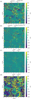 |
Fig. 9 Difference maps for vvlos (in m s−1). From top to bottom: Difference between reference map and straight VTF map; same for straight normalised VTF map; difference from first snapshot (snap1) to second snapshot (snap2); same for eleventh snapshot (snap11). |
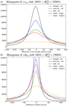 |
Fig. 11 Histograms of difference maps for line-of-sight velocity, ∆vlos, in upper panel a and the vertical component of the magnetic field strength, ∆Blos, in lower panel b. The histograms include pixels that have |

4.5 Error quantification
In order to quantify the visual impression of the difference maps, we compute histograms and plot them in Fig. 11. As the deviations are largest in the inter-granular lanes and in the filigree (magnetic) regions, we consider only pixels in which the vertical line-of-sight field strength of the reference map exceeds 100 G. We ignore 67 pixels with Blos > 2500 G as outliers. The histograms then include 25% of the pixels (i.e. 146 529 out of 589 824 pixels). The different line colours correspond to the different cases (see figure caption).
(straight VTF–reference) → red line
(normalised straight VTF–reference) → blue line
(rabbit VTF–reference) → green line
(snapshot 1–snapshot 2) → black line
(snapshot 1–snapshot 11) → yellow line.
The histograms of the vlos maps are plotted with a bin width of 10 m s−1 in Fig. 11a. The distributions peak close to vanishing differences. The peak height and the width are a quantitative measure for the measurement error: the larger the peak and the smaller the width, the smaller the measurement error. The visual impression of Fig. 9 is reflected in the distributions in terms of peak height and width: snap 1-snap 2 has the largest peak and the smallest width (i.e. the smallest errors), and snap 1–snap 11 has the smallest peak and the largest width (i.e. the largest errors). The histogram normalised straight-reference indicates smaller errors than straight–reference. It is also seen that the performance of the rabbit mode (green line) is not better than the straight mode (red line).
The histograms of the Blos maps are plotted with a bin width of 5 G in Fig. 11b. Again, the black line (snap 1–snap 2) has the largest peak (at 30521). The ordinate is clipped at a value of 12 000 to increase the visibility of the blue line (normalised straight) and the red line (straight). These two distributions peak at 11 716 and 10 177, respectively (i.e. again, the normalised straight mode performs better than the straight mode). The green line (rabbit mode) is worse and has a peak at 8263. As expected the differences between snap 1 and snap 11 are the largest such that the central peak of smallest differences only occurs 4276 times.
The histogram distributions in Fig. 11 are not Gaussian. In a Gaussian distribution, 68.27% of all values would lie within one standard deviation, 1σ (i.e. the full width including 68.27% corresponds to 2 · σ), and at that level the peak value is reduced by a factor of 1.65. Analogously, we determine the width, wfull, of the distribution that include 68.27% of all values, and then quantify the error as 1σ:= wfull/2.
These wfull/2 values are given in Tables 1 and 2 for vlos and Blos, respectively. We determine the distribution widths for four different mask criteria: all pixels (first column), pixels with 0 < |Blos| < 0.1 kG (second column, 75%), pixels with 0.1 < |Blos| < 2.5 kG (third column, 25%), pixels with 0.2 < |Blos| < 2.5 kG (fourth column, 20%).
Half of full distribution width, wfull/2, corresponding to 1σ, for difference maps of vlos in m s−1.
Half of full distribution width, wfull/2, corresponding to 1σ, for four different binning cases using the Blos-mask 0.1–2.5 kG.
4.5.1 Errors in vlos maps
The Doppler shift sensitivity of VTF was estimated (see Sect. 2) to be approximately 80 m s−1. This includes the noise level. The 1σ value of the straight mode is 1σ = 67 m s−1 if no mask is applied, which is of the same order of magnitude as the VTF sensitivity. For magnetic pixels (last two columns in Table 1), the 1σ error is more than double the size of the noise level: 1σ = 182 m s−1 for Blos > 100 G and 201 m/s for Blos > 200 G. Hence, the 1σ errors from solar evolution are substantial for a measurement span of 11 s.
In the normalised straight mode, the 1σ error decreases substantially by roughly a factor of two: 1σ = 36 m s−1, if no mask is applied, 88 m s−1 for Blos > 100 G, and 94 m s−1 for Blos > 200 G. The errors of the rabbit mode are slightly better than those of the straight mode, but not as small as those of the normalised straight mode.
Comparing the errors of snap 1 – snap 2 and snap 1 – snap 11 demonstrates that the temporal evolution is significant. The differences between the first two snapshots are small, much smaller than the VTF sensitivity. They are probably mostly caused by the low spectral resolution which does not allow for a more accurate determination. However, the errors between the first and the eleventh snapshot increase by a factor of eight or more: from 1σ = 18 m s−1 to 195 m s−1 for all pixels, and from 1σ = 50 m s−1 to 433 m s−1 for the pixels with Blos > 100 G.
We also computed the histograms for spatially binned data and list the results in Table 3 for the magnetic pixels with Blos between 0.1 and 2.5 kG. We find that the 1σ errors of the straight mode decreases from 1σ = 181 m s−1 for no binning, to 1σ = 169 m s for two by two binning, to 1σ = 148 m s−1 for four by four binning. Hence, even with a four by four binning the time-evolution error exceeds significantly the VTF sensitivity if the measurement is done in the straight mode. A four by four binning would correspond to the diffraction limit of a 1m aperture telescope.
It should be noted that if the measurement objective is to measure only velocities and not magnetic fields, the non-polarimetric Doppler mode can be chosen in which one accumulation is enough to measure the Stokes I line profile. This measurement only takes 0.9 s (VTF IPC, v.3.4, see Sect. 2), and deviations due to solar evolution can be safely neglected.
4.5.2 Errors in Blos maps
In Table 2, the error values characterising the distribution of the ΔBlos map are listed. These errors are to be compared to the VTF measurement sensitivity of 20 G, which results from the photon noise (see Sect. 2). It is seen that the 1σ errors for the entire map and for weak-field pixels (< 100 G) are negligible for straight and normalised straight modes. However, within the magnetic filigree the time-evolution errors are substantial. Considering all pixels with Blos between 100 and 2500 G, the error amounts to 48 G in the straight mode and to 36 G in the normalised straight mode, which is significantly larger than the 20 G error due to noise. Interestingly, the rabbit mode has an error of 84 G, and thus performs worse than both the straight and the normalised straight mode. It seems that the Milne-Eddington inversion can deal better with profiles where the neighbouring wavelength points are recorded close in time. It is not straightforward to explain this behaviour.
The differences between two consecutive snapshots (1 and 2) are negligible and smaller than 20 G in all cases. The time evolution is well reflected in the differences between the first and the eleventh snapshot (1 and 11). These differences correspond to an error of 1σ = 91 G for the magnetic pixels exceeding 100 G. Hence, for filigree and magnetic features which are shuffled around in the inter-granular lanes, the fields are strong enough, and more accumulation and longer effective exposure times will not improve the measurement. Due to their dynamic behaviour and strong fields, it may even be better to measure them with fewer accumulations (i.e. shorter effective exposure times). To measure magnetic fields in and above granules, the situation is different: the evolution timescale is longer and the magnetic fields are weaker. Hence, for granular magnetic fields more accumulations might be wanted to improve the S/N. However, one should be aware that a homogeneous horizontal field of 100 G produces a Q-amplitude of only some 0.0017 for Fe I 617.3 nm.
4.6 Implication for data pipelines
We have seen that the errors due to solar evolution can in all cases be reduced by normalising the continuum intensity to the instantaneous continuum intensity during the measurement as indicated by Eq. (1). This can be done in our case because we compute the whole line profile and its continuum for each snapshot. However, a Fabry–Perot instrument measures only one wavelength point at a time.
Instruments like VTF, CRISP, CHROMIS, and IBIS simultaneously measure a broad-band image at a neighbouring wavelength. These broad-band images can be used to mimic the temporal variation of the continuum intensity. To our knowledge, this is not currently done in existing Fabry–Perot data pipelines.
In order to apply Eq. (1), one needs to scale the broadband images to the continuum intensity of narrow-band images. As seen in Fig. 3, a complication may arise if a true continuum wavelength point is not part of the measurement sequence. Hence, in practise two approaches could do the job. The first is to add one more wavelength point to include a true continuum point outside the line. This point can then be used to determine the scaling factor between the broad-band intensity and the narrow-band continuum intensity. In the second approach, if the continuum intensity cannot be measured, for example because the line is too broad for the narrow pre-filter6, it is necessary to compute the average measured profile of a quiet-Sun region, fit a quiet-Sun profile to it, and determine the continuum intensity from the fitted profile to scale the broad-band intensities.
5 Conclusions
We investigated the measurement errors that arise due to temporal changes during the measurement process. Already with the 1.5 m telescope GREGOR (see Fig. 1), it could be seen that magnetic features in inter-granular lanes are shuffled around on a timescale of 11 s. This was also seen in the MURAM numerical simulations of a region with a mean vertical field strength of 200 G (see Fig. 5). Based on these simulations, we mimicked the measurement process of VTF and determined the measurement error by defining the truth to be the temporal average of the time that elapses during the measurement.
We find that granules are less affected and inter-granular areas with magnetic features are strongly affected. Depending on the science objective, it might be advisable to adapt the effective exposure time in the measurement. To measure strong fields in the inter-granular lane only a few accumulations may be enough, and would reduce the measurement error as the effective exposure time is reduced. For weaker fields within granules, more accumulations can be used as the evolution timescale is longer. For predominantly horizontal (perpendicular to line-of-sight) fields, more accumulations are necessary because the amplitude of linear polarisation in horizontal fields is much weaker than circular polarisation in vertical fields.
A key result of this investigation is the finding that a normalisation of the narrow-band intensities with the temporally averaged continuum intensity, following Eq. (1) (see Fig. 6 for an illustration), leads to a significant reduction in the measurement errors. In Sect. 4.6, we discuss how this normalisation could be integrated in existing pipelines, taking advantage of the simultaneously measured broad-band image.
Acknowledgements
We thank Matthias Rempel for providing the MURAM simulations, and Markus Schmassmann for making the data accessible and software to read the data. We thank Philip Lindner for providing the GREGOR data used in Sect. 1.
References
- Berkefeld, T., Schmidt, D., Soltau, D., von der Lühe, O., & Heidecke, F. 2012, Astron. Nachr., 333, 863 [NASA ADS] [CrossRef] [Google Scholar]
- Borrero, J. M., & Kobel, P. 2012, A&A, 547, A89 [NASA ADS] [CrossRef] [EDP Sciences] [Google Scholar]
- Borrero, J. M., & Kobel, P. 2013, A&A, 550, A98 [NASA ADS] [CrossRef] [EDP Sciences] [Google Scholar]
- Borrero, J. M., Tomczyk, S., Kubo, M., et al. 2011, Sol. Phys., 273, 267 [Google Scholar]
- Collados, M., López, R., Páez, E., et al. 2012, Astron. Nachr., 333, 872 [Google Scholar]
- Denker, C., Kuckein, C., Verma, M., et al. 2018, ApJS, 236, 5 [NASA ADS] [CrossRef] [Google Scholar]
- Dominguez-Tagle, C., Collados, M., Lopez, R., et al. 2022, J. Astron. Instrum., 11, 2250014 [NASA ADS] [CrossRef] [Google Scholar]
- Graham, J. D., Norton, A., López Ariste, A., et al. 2003, in Solar Polarization, eds. J. Trujillo-Bueno, & J. Sanchez Almeida, Astronomical Society of the Pacific Conference Series, 307, 131 [NASA ADS] [Google Scholar]
- Jurčák, J., Collados, M., Leenaarts, J., van Noort, M., & Schlichenmaier, R. 2019, Adv. Space Res., 63, 1389 [Google Scholar]
- Kaithakkal, A. J., Borrero, J. M., Fischer, C. E., Dominguez-Tagle, C., & Collados, M. 2020, A&A, 634, A131 [EDP Sciences] [Google Scholar]
- Kentischer, T. J., Schmidt, W., & Sigwarth, M. 2012, VTF: ETALONS, Tech. Rep. VTF-Project Documentation: ATST-KIS-VTF-ET1000-TN-001, Leibniz-Institut für Sonnenphysik (KIS) [Google Scholar]
- Pastor Yabar, A., Borrero, J. M., & Ruiz Cobo, B. 2019, A&A, 629, A24 [NASA ADS] [CrossRef] [EDP Sciences] [Google Scholar]
- Rempel, M. 2014, ApJ, 789, 132 [Google Scholar]
- Rimmele, T. R., Warner, M., Keil, S. L., et al. 2020, Sol. Phys., 295, 172 [Google Scholar]
- Schmidt, W., von der Lühe, O., Volkmer, R., et al. 2012, Astron. Nachr., 333, 796 [Google Scholar]
- Schmidt, W., Bell, A., Halbgewachs, C., et al. 2014, SPIE Conf. Ser., 9147, 91470E [NASA ADS] [Google Scholar]
- Schmidt, W., Schubert, M., Ellwarth, M., et al. 2016, SPIE Conf. Ser., 9908, 99084N [NASA ADS] [Google Scholar]
- Schubert, M. J. 2016, Ph.D. thesis, Albert Ludwigs University of Freiburg, Germany [Google Scholar]
- Schubert, M., Kentischer, T., & von der Lühe, O. 2017, J. Astron. Telescopes Instrum. Syst., 3, 1 [CrossRef] [Google Scholar]
- Sigwarth, M. 2017, VTF Etalon 1 Coating and Stress Compensation Processing. VTF Technical Note ATST-KIS-VTF-ET1000-TN-016, Tech. rep., Kiepenheuer-Institut für Sonnenphysik (KIS) [Google Scholar]
- Stix, M. 2002, The Sun: An Introduction, 2nd edn. (Berlin, Heidelberg: Springer-Verlag) [Google Scholar]
- Wöger, F., von der Lühe, O., & Reardon, K. 2008, A&A, 488, 375 [NASA ADS] [CrossRef] [EDP Sciences] [Google Scholar]
At first light, VTF will be equipped with only one FPI (also named etalon), but the second FPI is manufactured and will be integrated soon after the first.
This line has very similar properties to the iron lines at 630 nm and at 525.0 nm (Graham et al. 2003). Initially, the intention of this work was to compare VTF measurements with HMI on board SDO. The focus changed, and we continued to use Fe 1617.3 nm. Fe 1617.3 nm has the advantage of being surrounded by a clean continuum.
The pre-filter is needed to suppress side peaks from the etalon(s).
All Tables
Half of full distribution width, wfull/2, corresponding to 1σ, for difference maps of vlos in m s−1.
Half of full distribution width, wfull/2, corresponding to 1σ, for four different binning cases using the Blos-mask 0.1–2.5 kG.
All Figures
|
Fig. 1 Speckle-reconstructed images of a filigree region close to disc centre observed with HiFi at GREGOR on June 30, 2019, in G band at 430 nm. The upper large panel shows a large FOV at 08:22:21 UT. The four small lower panels show four subsequent snapshots t = 0, 11, 23, and 35 s of a smaller FOV (white box in upper panel). The tick marks indicate units in arcsec. |
| In the text | |
|
Fig. 2 MURAM simulation snapshot. (a) Vertical cut through numerical box showing the modulus of the magnetic field strength in logarithmic scale, clipped between 10 and 2500 G, with the colour bar in logarithmic scale. (b) Horizontal cut at mean temperature of 5560 K of vertical velocity in km s−1 with positive values pointing upwards (being blue-shifted to observer). (c) Same as panel b, but for the vertical component of the magnetic field strength in kG. |
| In the text | |
|
Fig. 3 Stokes I, Q, U, and V profiles (from upper left to lower right). The red line denotes synthesised profiles with intrinsic sampling of 0.4 pm. The green line in the lower left panel sketches the shape of the VTF transmission curve. Blue crosses and lines mimic 11 VTF measurement points as a result of convolving the synthetic profiles with the VTF transmission curve. |
| In the text | |
|
Fig. 4 Example pixel of the Stokes profiles for t = 0 s (blue) and t = 10 s (red) is plotted. The black curve shows the profile from a temporal average of all 11 snapshots. |
| In the text | |
|
Fig. 5 Change of continuum intensity during line scan. Upper panel: continuum image with intensities between 0.6 and 1.45 for the first snapshot. The average intensity is normalised to one. Lower panel: difference between the continuum images of snapshot 1 and snapshot 11. The difference map is clipped at differences of ±10%. |
| In the text | |
|
Fig. 6 Comparison of Stokes I and V profiles in upper and lower panel, respectively: Straight composed (red) simulating the VTF measurement, straight normalised (blue), and time-average. The green line in the upper panel denotes the continuum intensity at each wavelength (=time) step. |
| In the text | |
|
Fig. 7 Maps for line-of-sight velocity, vlos (upper panel), and vertical component of the magnetic field strength, Blos (lower panel), inverted with VFISV from reference (time-averaged) Stokes profiles. As these maps are simulated observables, arcsec are used instead of km for the spatial dimension. |
| In the text | |
|
Fig. 8 Histograms for maps of line-of-sight velocity with a bin size of 115 m s−1 (upper panel), and vertical component of the magnetic field strength with a bin size of 30 G (lower panel) for the inverted maps of the reference (time-averaged) profiles. |
| In the text | |
|
Fig. 9 Difference maps for vvlos (in m s−1). From top to bottom: Difference between reference map and straight VTF map; same for straight normalised VTF map; difference from first snapshot (snap1) to second snapshot (snap2); same for eleventh snapshot (snap11). |
| In the text | |
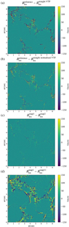 |
Fig. 10 Same as Fig. 9, but for Blos (in gauss). |
| In the text | |
|
Fig. 11 Histograms of difference maps for line-of-sight velocity, ∆vlos, in upper panel a and the vertical component of the magnetic field strength, ∆Blos, in lower panel b. The histograms include pixels that have |
| In the text | |
Current usage metrics show cumulative count of Article Views (full-text article views including HTML views, PDF and ePub downloads, according to the available data) and Abstracts Views on Vision4Press platform.
Data correspond to usage on the plateform after 2015. The current usage metrics is available 48-96 hours after online publication and is updated daily on week days.
Initial download of the metrics may take a while.