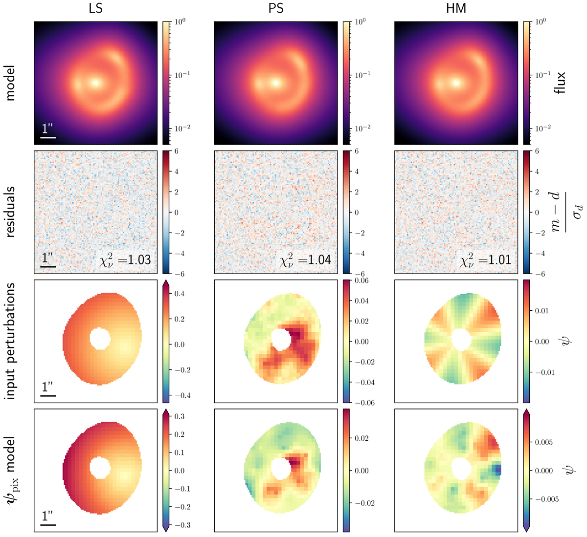
Best-fit pixelated potential reconstruction of our simulated data set, assuming all other model components are perfectly known. Each column represents the different types of perturbations considered in this work. From top to bottom: simulated data, image model, normalized residuals, input perturbations, ψ_pix model. The outlined annular region on the potential panels corresponds to the solid lines in the panels of Fig. 3, and is where the S/N of the lensed source is higher than 5. Perturbations outside this area are cropped only to ease the visual comparison with the input perturbations (there is no cropping or masking during modeling). Additionally, for lens LS only, the minimum value of the perturbations is subtracted from the model, again to ease the comparison with the input SIS profile (this does not affect the lensing observables). An animated visualization of the gradient descent optimization is available https://obswww.unige.ch/ galanay/animations/.