| Issue |
A&A
Volume 668, December 2022
|
|
|---|---|---|
| Article Number | A72 | |
| Number of page(s) | 12 | |
| Section | Atomic, molecular, and nuclear data | |
| DOI | https://doi.org/10.1051/0004-6361/202244043 | |
| Published online | 07 December 2022 | |
Dielectronic recombination data for dynamic finite-density plasmas
XVI. The phosphorus isoelectronic sequence
1
Department of Physics, Marmara University, Ziverbey,
Istanbul
34722, Turkey
e-mail: This email address is being protected from spambots. You need JavaScript enabled to view it.
2
Department of Physics, University of Strathclyde,
Glasgow
G4 0NG, UK
Received:
17
May
2022
Accepted:
11
September
2022
Abstract
Dielectronic (DR) and radiative (RR) recombination rate coefficients for 19 phosphorous-like ions, between S+ and W59+, forming sulphur-like ions, have been calculated as part of the assembly of a level-resolved database necessary for modelling dynamic finite-density plasmas, within the generalized collisional-radiative framework. Calculations have been performed within the multi-configuration Breit-Pauli approximation using the code AUTOSTRUCTURE, from both ground and metastable initial states, in both LS coupling and intermediate coupling (IC), allowing for ∆n = 0 and ∆n = 1 core-excitations from the ground and metastable levels involved in the DR processes. Partial and total DR coefficients have been calculated for S+ to Zn15+, as well as Kr21+, Mo27+, Xe39+, and W59+. Results for a selection of ions from the sequence are discussed in this paper, and are compared with the existing theoretical and experimental results. Dielectronic recombination results for the Fe11+ resonance spectrum associated with ∆n = 0 core excitations are compared with those from merged-beam measurements. Fits to the total (IC) DR and RR rate coefficients are presented in tabular form. Partial LS and IC DR and RR rate coefficients are archived in the open access database OPEN-ADAS in standard ADAS adf09 and adf48 file formats, respectively.
Key words: atomic data / atomic processes
© E. A. Bleda et al. 2022
 Open Access article, published by EDP Sciences, under the terms of the Creative Commons Attribution License (https://creativecommons.org/licenses/by/4.0), which permits unrestricted use, distribution, and reproduction in any medium, provided the original work is properly cited.
This article is published in open access under the Subscribe-to-Open model. This email address is being protected from spambots. You need JavaScript enabled to view it. to support open access publication.
1 Introduction
Dielectronic recombination (DR) is the dominant electron-ion recombination process in most astrophysical and laboratory plasmas, as emphasized by Burgess (1964, 1965). In this process, a free electron can collisionally excite an ion and be simultaneously captured into a Rydberg level to form a recombined ion in a doubly excited state. Dielectronic recombination occurs if the resulting doubly excited state subsequently decays radiatively below the first ionization threshold. Radiative recombination (RR) is another process by which free electrons are recombined with the ions in the plasma through pure radiative transitions. The DR process is largely responsible for the emission lines seen at discrete frequencies in a plasma spectrum, which are of great importance for plasma temperature diagnostics (Gabriel 1972). Radiative recombination gives rise to a continuum of emission, with a minimum energy equal to the binding energy of the ion in its final state. The DR and RR processes have major influences on the formation of the ion charge-state distributions of collisionally ionized and photoionized plasmas, respectively (Hahn 1997; Del Zanna & Mason 2018).
Astrophysical and laboratory plasmas can broadly be classified as collisionally ionized or photoionized plasma, depending on the type of processes responsible for the thermal and ionization balance of their sources. In a collisionally ionized plasma, ionization takes place mainly through the collision of electrons with the ions of the plasma. The average thermal energies of free electrons in a collisionallly ionized plasma are usually on the same scale as the ionization energies of the ions in the plasma, as result of which the DR rates get contribution from both ∆n = 0 and ∆n ≥ 1 excitations (Savin et al. 1997; Nahar & Pradhan 1997). Dielectronic recombination is the primary process for achieving ionization balance in collisionally ionized plasmas, typically for temperatures greater than ~106 K. Stellar corona, supernova remnants, and gas in galaxies or in clusters of galaxies are some examples of astrophysically important collisionally ionzed space plasmas (Bryans et al. 2006, 2009).
Photoionized plasmas are widespread in space. Active galactic nuclei, X-ray binaries, and cataclysmic variables are some examples treated in this domain. The DR rates for a photoionized plasma are almost entirely determined by ∆n = 0 excitations from the fine-structure resolved ground states of the ions (Savin et al. 1997; Bryans et al. 2006). To determine the level populations and ionization balance of such plasmas, one needs to know the rates characterizing all the relevant atomic and, sometimes, molecular processes occurring in them. The DR and RR rates that characterize the recombination and ionization processes occurring in most types of astrophysical and laboratory plasmas are among the most important atomic data used in the design of multi-parameter models for the structural diagnosis of both collisional and photoionized plasmas (Badnell et al. 2003; Müller 2008; Fritzsche 2021; Mendoza et al. 2021).
The coronal approximation is often used to model the low-density astrophysical plasmas to determine the ionization balance and understand the emission properties. However, the coronal approximation breaks down as the particle density increases. Then, one needs final-state resolved partial DR and RR rate coefficients to carry out collisional-radiative population modelling (Bates et al. 1962; Summers et al. 2006; Burgess & Summers 1969).
Codes developed mainly for modelling collisional ionized plasmas include Mekal (Mewe et al. 1995), SPEX (Kaastra et al. 1996), XSPEC (Arnaud 1996), APEC (Smith et al. 2001), CHIANTI (Del Zanna et al. 2021), and ADAS (Summers 2004). Codes developed mainly for modelling the photoionized plasma include CLOUDY (Ferland et al. 1998), XSTAR (Mendoza et al. 2021), and MOCASSIN (Ercolano et al. 2007).
The need for DR and RR rates for spectroscopic modelling of plasmas in ionization equilibrium and non-equilibrium was described by Badnell et al. (2003). Their paper also laid down the groundwork for a large-scale collaborative project known by the name Atomic Processes for Astrophysical Plasmas (APAP1), to calculate total and final-state level-resolved DR and RR rate coefficients from both the ground and the metastable states of the isoelectronic sequences of the elements of the periodic table relevant to the modelling of astrophysical and laboratory plasmas. Many papers in the literature have presented DR and RR results calculated in both LS coupling and intermediate coupling (IC) within the multi-configuration Breit-Pauli (MCBP) approximation, as implemented in the collision code known by the name AUTOSTRUCTURE (Badnell 1986, 1997, 2011) as part of the APAP project. The completed isoelectronic sequences that have appeared in the literature include hydrogen-like (Badnell 2006a), helium-like (Bautista & Badnell 2007), lithium-like (Colgan et al. 2004), beryllium-like (Colgan et al. 2003), boron-like (Altun et al. 2004), carbon-like (Zatsarinny et al. 2004b), nitrogen-like (Mitnik & Badnell 2004), oxygenlike (Zatsarinny et al. 2005, 2003), fluorine-like (Zatsarinny et al. 2006), neon-like (Zatsarinny et al. 2004a), sodium-like (Altun et al. 2006), magnesium-like (Altun et al. 2007), argon-like (Nikolić et al. 2010), aluminium-like (Abdel-Naby et al. 2012), and the silicon-like (Kaur et al. 2018) sequences. Complementary comprehensive calculations for RR rate coefficients were done from the initial ground and metastable levels of all elements up to and including Zn, plus Kr, Mo and Xe, for all isoelectronic sequences up to Na-like ions forming Mg-like ions (Badnell 2006d). The benchmarking work done for the DR of Fe13+ as M-shell ions (Badnell 2006c) provided much information about the underlying mathematical methodology to challenge more complex cases involving M-shell ions.
The main purpose of this work is twofold: the first is to provide systematically calculated DR and RR rates for the phosphorous(P)-like isoelectronic sequence from S to Zn, along with Kr, Mo, Xe, and W elements of the periodic table as basic ingredients for the physical and spectral diagnostic modelling of astrophysical and laboratory plasmas, in general. The second is more specific and arises from the need for the spectroscopic atomic data that characterizes the excitations from iron-M shell ions for the analysis of the spectral emission recorded by Sako et al. (2001, 2003) and Holczer et al. (2009). Calculations have been carried out over a wide range of electron temperatures, Z2(10–107) K, where Z is the target ion charge. Both Δn = 0 and Δn = 1 core excitations involving 3s and 3p sub-shells occurring during the capture of the colliding electron are considered in the calculations.
The remainder of this paper is organized as follows: In Sect. 2, we give a brief description of the structures and methodologies used. In Sect. 3, we compare merged-beam measured recombination rate coefficients by Novotnỳ et al. (2012) for Fe11+ with the results of our calculations in the region of energies where the dominant contributions to DR rates come from the autoionization resonances associated with the 3s → 3p and 3p → 3d core excitations. In Sect. 4, we discuss the DR and RR rate coefficients calculated for all ions considered in this work. We then compare our total DR and RR rate coefficients, and compare them with the corresponding merged-beam measured Maxwellian recombination rate coefficients for Fe11+ and with the recent results of Dufresne et al. (2021) for S+. Section 5 concludes with a brief summary.
2 Methodologies
The complex and challenging nature of the problem requires us to be clear in both the mathematical theory and the structures used to describe the initial and recombined target states involved in the DR and RR processes. We provide the main equations used to calculate the partial level-resolved DR and RR rates for a selected number of temperatures, along with equations extending the total rates to any temperatures desired.
2.1 Theory
The theoretical basis of our calculations has already been given in Badnell et al. (2003) and Badnell (2006c). We used AUTOSTRUCTURE2 (Badnell 2011) with the most recently updated suites of codes. We used AUTOSTRUCTURE (Badnell 1986) to carry out multi-configuration Breit-Pauli calculations for all the necessary rates and energies needed to calculate the DR and RR rate coefficients in the independent processes, isolated resonance, distorted-wave (IPIRDW) approximation, which neglects the interference between DR and RR process. Pindzola et al. (1992) studied the interference between DR and RR processes in detail using higher-order perturbation theory and analysed it quite generally. It was found that the interference has a first-order effect (in 1/q, where q is the Fano q-factor) as an asymmetry in the line profile, as seen in high-resolution photoionization measurements. However, when the total cross section is averaged over the resonance line profile, the first-order effect vanishes identically – see also Badnell & Pindzola (1992) and Behar et al. (2000). So, it is the second-order effect (in 1/q2) on the energy-averaged total cross section and on the corresponding Maxwellian rate coefficient. Then they considered the entire parameter space and showed quite generally that for all practical purposes the interference contribution to the energy-averaged total cross section is negligible and can safely be neglected for plasma modelling. We should also note that the IPIRDW approximation readily enables an analytic integration over the resonance profiles to get the energy-averaged cross sections needed to calculate the corresponding DR rates. Energy levels, radiative rates, and autoionization rates were calculated in both LS and IC approximations using non-relativistic radial orbitals up to Zn and kappa-averaged relativistic radial functions thereafter.
The dielectronic recombination process involving the ground-state electron configuration of a P-like ion X, with a degree of ionization q, can be represented schematically as
![Mathematical equation: ${{\rm{e}}^ - } + {X^{{q^ + }}}\left( {3{{\rm{s}}^2}3{{\rm{p}}^3}\left[ {^4{{\rm{S}}_{3/2}}} \right]} \right) \to {X^{\left( {q - 1} \right) + **}} \to {X^{\left( {q - 1} \right) + }} + hv,$](/articles/aa/full_html/2022/12/aa44043-22/aa44043-22-eq1.png) (1)
(1)
where X(q−1)+** represents the doubly excited intermediate resonance states formed upon the capture of the incoming electron by the target ion Xq+, and hv is the photon energy. If the last step X(q−1) + hv of a DR process represented by Eq. (1) results in one step through a direct recombination of an incident electron on the ground state, then the process is referred to as RR. The RR process can take place at any collision energy with finite probabilities for recombination to all available levels of the recombined ion, while the DR process can take place only if the total energy of the incoming free electron is equal to the difference of the total energies of the final doubly excited states and the initial states of the target ion.
The partial DR rate coefficients  , from an initial metastable state i, into a final recombined state v, schematically represented by Eq. (2), is given in the IPIRDW approximation as described by Burgess (1964):
 (2)
(2)
where the outer sum is over all accessible (N + 1)-electron doubly excited resonance states j, ωj is the statistical weight of the state j, and ωv is the statistical weight of the N-electron target state. The statistical weight, ω, is defined as (2L + 1)(2S + 1) in LS and (2J + 1) in IC. Aa and Ar are the autoionization and radiative rates in inverse seconds, respectively. Here, Ec is the energy of the continuum electron of angular momentum l, which is fixed by the position of the resonances, IH is the ionization potential energy of the hydrogen atom, kB is the Boltzmann constant, a0 is the Bohr radius, Te is the electron temperature, and  cm3. The summation over h accounts for all possible bound and autoionizing states. The sum over m includes the autoionization to states other than the initial state i.
Detailed balanced is used to calculate the partial RR rate coefficients  is given below:
![Mathematical equation: $\matrix{{\alpha _{fv}^{{\rm{RR}}}\left( {{T_{\rm{e}}}} \right)} \hfill & = \hfill & {{{c{\alpha ^3}} \over {\sqrt \pi }}{{{\omega _f}} \over {2{\omega _v}}}{{\left( {{I_{\rm{H}}}{k_{\rm{B}}}{T_{\rm{e}}}} \right)}^{ - 3/2}}} \hfill \cr {} \hfill & {} \hfill & { \times \int_0^\infty {E_{vf}^0\sigma _{vf}^{{\rm{PI}}}\left( E \right)\exp \left[ { - {E \over {{k_{\rm{B}}}{T_{\rm{e}}}}}} \right]{\rm{d}}E} ,} \hfill \cr}$](/articles/aa/full_html/2022/12/aa44043-22/aa44043-22-eq6.png) (3)
(3)
where  represents the corresponding photoionization cross section in cm2 for the inverse processes, Evf is the photon energy emitted during the RR process, and
  cm s−1 (Preval et al. 2016).
During the capture of the incoming electron by the target ion there could be Δn = 0 intra-shell or Δn ≥ 1 inter-shell core electron excitations. In this work, only DR processes associated with Δn = 0 and Δn = 1 cases are considered.
In order to facilitate their use, we fit our total DR rate coefficients using the equation
 (4)
(4)
where n takes on different values depending on the target ion. Here, T and Ei are in units of temperature (K) and the rate coefficient αDR is in units of cm3 s−1.
Also, the total RR rate coefficients are computed and fitted using the formula of Verner & Ferland (1996):
![Mathematical equation: ${\alpha ^{{\rm{RR}}}}\left( T \right) = A\sqrt {{{{T_0}} \over T}} {\left[ {{{\left( {1 + \sqrt {{T \over {{T_0}}}} } \right)}^{1 - B}}{{\left( {1 + \sqrt {{T \over {{T_1}}}} } \right)}^{1 + B}}} \right]^{ - 1}},$](/articles/aa/full_html/2022/12/aa44043-22/aa44043-22-eq10.png) (5)
(5)
where for low-charge ions, we replace B by Gu (2003):
 (6)
(6)
Here the fit parameters T0,1,2 are in the units of temperature (K), the fit parameters B and C are dimensionless, and the parameter A has the unit of the RR rate coefficients αRR, which is cm3 s−1. A non-linear least-squares fit was used to determine the coefficients A, B, C, and T0,1,2.
2.2 Nomenclature and structures
The process in which the incoming electron is captured into any one of the empty 3l(l = 0–2) orbitals of the ground complex while simultaneously causing Δn = 0 intra-shell core excitations within it will be referred to as the 3 → 3, 3 process. The process in which the incoming electron is captured into a Rydberg orbital nl (n > 3) accompanied by Δn = 0 intra-shell core excitations within the n = 3 shell will be referred to as the 3 → 3, n process. The process in which the incoming electron is captured into any of the 4l (l = 0–3) Rydberg orbitals, simultaneously causing Δn = 1 inter-shell core excitations from the n = 3 to n = 4 shell, will be referred to as the 3 → 4, 4 process. The labelling 3 → 4, n will be used to represent the process in which the incoming electron is captured to nl (n > 4), simultaneously causing Δn = 1 inter-shell core excitations from n = 3 to n = 4.
To calculate the DR rate coefficients involving the 3 → 3, 3 and 3 → 3, n processes, the configuration interaction (CI) expansion for the initial state of P-like ions considered in this work is represented by the basis set consisting of the 3s23p3, 3s23p23d, 3s3p4, 3s3p33d, 3s23p3d2, 3s3p23d2, 3p5, and 3p43d configurations, where an assumed closed-shell Ne-like core is omitted from the labelling. It is important to notice that all these configurations can be derived from the ground-state configuration 3s23p3 through intra-shell (Δn = 0) single and double electron promotions (core excitations) within it. In the rest of the paper, these configurations will be referred to as N-electron configurations. The resulting configuration interaction state wave functions are computed using optimized single-electron orbitals generated from a scaled Thomas-Fermi–Dirac–Amaldi (TFDA) model potential (Eissner & Nussbaumer 1969), including the mass-velocity and Darwin relativistic corrections as implemented in AUTOSTRUCTURE. The scaling parameters λ3s, λ3p, and λ3d are optimized in a multi-configuration variational procedure, minimizing a weighted average of a selected number of LS term energies while keeping the radial scaling parameters for the 1s, 2s, and 2p closed-core orbitals fixed at their default values of 1.0. Term energies can be non-relativistic or kappa-averaged relativistic, including the effects of one-body Breit–Pauli (BP) effects.
Here we should note that AUTOSTRUCTURE DR and RR rate calculations performed previously (Badnell 2006b) for Fe11+ used Slater-type-orbital (STO) model potentials (Burgess et al. 1989) to generate the orbital basis, whereas for the present calculations, we used the Thomas-Fermi-Dirac-Amaldi (TFDA) model potential to generate the orbital basis for all cases. The electron configuration 3s 3p2 3d2 was also not included in the description of the initial state of Fe11+ in the previous calculations by Badnell (2006b), while it is included for all cases in the present calculations. It is found to have a large influence on the CI mixing of the terms and the levels of the electron configurations describing the target ions. It also greatly increases the number of capture channels for the incoming electron. The differences between the present and previous calculations for Fe11+ are described in the results section.
The electron configurations 3s2 3p4, 3s23p23d2, 3s3p43d, 3s3p23d3, 3p6, 3p43d2, 3s23p33d, 3s3p5, 3p53d, and 3s23p3d3 are used as the (N + 1)-electron excited intermediate resonance states generated through the 3 → 3, 3 processes for all P-like ions considered in this work. The (N + 1)-electron excited intermediate resonance states used for DR-calculations involving the 3 → 3, n process described above are constructed by coupling a Rydberg orbital, nl, or a continuum orbital, kl, to the N-electron target configurations described in the previous paragraph.
The N-electron configurations used to describe the target CI state for the 3 → 4 processes are 3s23p3, 3s23p23d, 3s23p24l, 3s3p4, 3s3p33d, and 3s3p34l, where l = 0-3. The (N + 1)-electron autoionizing states used for the DR calculations involving the 3 → 4, 4 processes are 3s23p24l4l′ and 3s3p34l4l′ with l(l′) = 0–3. The (N + 1)-electron excited intermediate resonance states used for DR calculations involving the 3 → 4, n process are generated by coupling a Rydberg orbital, nl, or a continuum orbital, kl, to the N-electron target configurations of the 3 → 4 process as given above.
Distorted wave calculations are performed to generate the bound nl and continuum kl orbitals needed for building the initial, intermediate, and the final states involved in the calculations of DR and RR rates. For the ∆n = 0 and 1 cases, l values are included up to 11 and five, respectively. The corresponding n-values are all those up to 25, followed by a set of representative values up to 999. For large values of n, the bound Rydberg orbital is approximated by a zero-energy continuum orbital utilizing quantum-defect theory (Badnell et al. 2003).
The wave functions constructed using these (N + 1)-electron basis configurations discussed above are used to determine the autoionization and radiative rates, which are then assembled to obtain the final state level-resolved and total dielectronic recombination and radiative rate coefficients for all P-like ions considered in this work.
3 Comparison of calculated Fe11+ DR resonance spectrum with experiment
Novotnỳ et al. (2012) measured electron-ion recombination rate coefficients for Fe11+ forming Fe10+ using amerged-beam set-up at the heavy-ion Test Storage Ring (TSR) located at the Max Planck Institute for Nuclear Physics in Heidelberg, Germany. The eight configurations used to represent the initial quantum state of P-like target ions considered in this work are constructed by allowing single and double electron promotions from the lowest-order ground-state configuration containing a valance half open p-shell, as detailed in the theory section. Such a description of the initial state of the DR process of any P-like ions makes the resulting DR resonance spectrum very complex and almost impossible to label the individual features in it with clarity. Therefore, in this section, we do our best to at least identify the three strong ground core dipole-excited resonance series converging to their respective thresholds.
To compare our IC DR calculation for Fe11+ with the experiment, we convoluted our ∆n = 0 DR energy-averaged cross sections (× velocity) with the energy spread corresponding to temperatures kBT± = 12.00 meV and kBT‖ = 0.09 meV with and without the field ionization effects. To account for the field ionization effects, each nl partial DR cross section was multiplied by the relevant survival probability (Schippers et al. 2001), as were also used in the previous calculations by Badnell (2006b), as described in the paper by Novotnỳ et al. (2012).
The present IC DR rate coefficients calculated for Fe11+ are compared with the measured data in various panels of Fig. 1. The solid green curve represents the present IC DR rate coefficients.
The fourth panel of Fig. 1 compares our results with the corresponding results given in Fig. 2 of the paper by Novotnỳ et al. (2012). The solid green curve in this panel represents current results. The solid orange curve represents the previous calculation of Badnell (2006b). The solid blue curve with dots represents the merged-beam measurement. It is clearly seen that our current results match with the experiment between the energy range 25–60 eV better than the previous calculations.
The difference between the results with and without the field ionization becomes apparent only very near the 3s23p2 (3p)3d[4PJ] ionization thresholds, as seen from the last panel of Fig. 1 where the solid black curve reflects the field ionization effects. We also convoluted our ∆n = 0 DR cross sections (× velocity) with lower temperatures of values kBT± = 1.5 meV and kBT = 0.025 meV to see somewhat finer details (Novotnỳ et al. 2012; Lestinsky et al. 2008). The partial result from this calculation is depicted in the magenta curve of the first panel of Fig. 1 to illustrate the point. It should be noted that the magenta curve does not have any field effects.
The near-threshold bound or resonance states are formed by (N + 1)-electron configurations that result from the capture of incoming electron by the target ion. Such states not only have strong capture and radiative rates, but also they play major role in the low-temperature DR process (Nussbaumer & Storey 1983). Thus, the accurate energy positions of the low-lying doubly excited autoionizing states of the recombined ion are critically important for extracting reliable low-temperature DR rates from any model calculations. The inherent difficulties in calculating such energy positions relative to the respective ionization thresholds of the recombined ion accurately enough may result in significant uncertainties in the near-threshold rate coefficients. With this in mind, for ∆n = 0 core-excitations, the resonance energies for the first 46 levels are empirically adjusted so that the corresponding series limits match the 3 → 3 core-excitation energies obtained from the NIST3. We made semi-empirical adjustments for those level energies that are missing from the NIST tables. We did so by comparing our calculated energies for them with our calculated energies for levels that are present in the NIST tables. We then applied similar shifts to the former calculated level energies as we made to the latter. The energies with asterisks (*) in Table 1 are the estimated observed energies.
Low-lying DR resonances associated with the autoionization of doubly excited states to the ground state of the Fe11+ target ion are labelled in the consecutive panels of Fig. 1. There are about 83 200 overlapping resonances in total emanating from the autoionization of doubly excited states energetically above the various other levels of the configurations used to describe the Fe11+ target ion. There are about 680 resonances in the very narrow energy range of the top panel of Fig. 1, as a result of which we obtain a smeared-out profile in the corresponding DR rate coefficients. The number of overlapping autoionizing resonances in the energy range of the second, third, and fourth panels of Fig. 1 are about 5050, 7900, and 69 500, respectively. Although the smearing-out of these resonances makes it very difficult to identify the individual lines, we label some of the most pronounced autoionizing resonances, leading to the series limits 3s23p3 [2DJ], 3s23p3 [2PJ], 3s3p4 [2P1/2], 3s3p4[4P5/2], and 3s23p2(3P)3d[4P5/2]. The peaks just above the resonances that lead to the series limit 3s23p2 (3P) 3d [4P5/2] with similar profiles, with varying sizes, are the autoionization resonances that lead to the series limits 3s23p2 (3P) 3d [4P3/2] and 3s23p2 (3P) 3d [4P1/2], respectively, as is clearly seen in the fourth panel of Fig. 1. Given the complexity of the problem, along with the possible uncertainties in the position of near-threshold resonances, the overall agreement between our IC resonance DR results with the experimental measurements of Novotnỳ et al. (2012) is quite good. Indeed, as we move away from the low-T region towards the high-T region, the agreement between theory and experiment improves further.
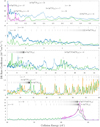 |
Fig. 1 Present IC DR rate coefficients for the ground state of Fe11+, as a function of centre-of-mass collision energy in the range 0 to 70 eV. This energy region is dominated by the ∆n = 0 core dipole-excited resonances; (a) the solid green curve denotes our IC results where energy-averaged DR cross sections (× velocity) have been convoluted with the experimental merged-beam electron energy distribution, characterized by the electron temperatures kBT⟘ = 12.00 meV and kBT = 0.09 meV (and without the field ionization effects); (b) the solid blue curve with dots denotes the measured merged-beam recombination rate coefficient by Novotnỳ et al. (2012); (c) the solid orange curve denotes the previous calculations by Badnell (2006b), as given Fig. 2 of the paper by Novotnỳ et al. (2012); (d) the solid black curve differs from the solid green curve only now that we include field ionization effects; (e) the solid magenta curve represents our IC DR rate coefficients with the convolution describing the electron beam energy spread according to somewhat lower temperatures, kBT⟘ = 1.5 meV and kBT = 0.025 meV. |
Energies (Ryd) of the Fe11+ target levels.
4 Results for total Maxwellian rate coefficients
Maxwellian-averaged total DR and RR rate coefficients calculated in both LS coupling and IC within the MCBP approximations, using the mathematical framework detailed in the theory section for all ions considered in this work, are compared with existing results from the literature in Figs. 2–5. All of our total DR and RR rates were fitted using Eqs. (4) and (5), respectively, and the resulting fitting coefficients in IC are listed in Tables 2 and 3. Our DR and RR fits reproduce the actual computed data to better than 5% for all ions over the temperature range Z2(101–107) K, where Z is the residual charge of the recombining ion.
We now show a series of comparisons. In all figures, we have denoted the temperature regions of collisionally ionized and photoionized plasmas by bars. The collisionally ionized zones for all ions considered in this work are determined by using the fractional abundances given in Bryans et al. (2009) and considering the range of temperatures for the ion’s fractional abundance is >90% of its maximum value. The photoionized zones are determined by using ion fractions and temperatures of an optically thin, low-density photoionized gas for S+, Ar3+, Ca5+, and Fe11+, as given by Kallman & Bautista (2001). The photoionized zones for ions for which Kallman & Bautista (2001) do not provide explicit ion fractions are determined by linear interpolation. We used Ar3+ and Ca5+ data for the photoionized zones of K4+ ions, and Ca5+ and Fe11+ data for the photoionized zones of Ti7+, V8+, Cr9+, and Mn10+ ions. The left side of the bars representing the photoionized zones are omitted when their extent is undetermined.
We used the recommended data set of Mazzotta et al. (1998), which is based on data from Shull & Van Steenberg (1982), Landini & Fossi (1991), and Mattioli (1988), as well as the Burgess (1965) general formula, to compare with our results. The calculations on which the recommended data of Mazzotta et al. (1998) were based were carried out for the ground state and often using single-configuration LS coupling approximations or semi-empirical formulae or isoelectronic interpolations without considering metastable initial states. There is a critical review of many of these studies and others in Savin & Laming (2002). Since we could only find results for Fe11+ and S+ ions, other than those of Mazzotta et al. (1998), we discuss these ions in detail first in Sects. 4.1 and 4.2.
Before discussing the results for Fe11+ and S+, it is useful to compare the AUTOSTRUCTURE MCBP oscillator strengths for the transitions that dominate the (high-T) DR with the corresponding results from the Breit-Pauli Multi-configuration Hartree-Fock (MCHF) calculations of Irimia & Froese Fischer (2005); Tayal & Zatsarinny (2010) for S+ and Froese Fischer et al. (2006) for Fe11+. The agreement shown in Table 4 between the present MCBP and Breit-Pauli MCHF results is very good in both cases. The accuracy of the core radiative rates for these transitions directly controls the accuracy of the high-temperature DR peak.
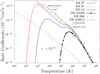 |
Fig. 2 Total Maxwellian-averaged DR and RR ground-state rate coefficients for Fe11+: (a) the solid black curve with small squares (DR MM98) represents the recommended DR rates extracted from the fitted coefficients of Mazzotta et al. (1998); (b) the solid red and blue curves represent our IC and LS DR rates, respectively; (c) the dashed red curve is our IC RR rates; (d) the dash-dotted magenta curve (DR B06) represents the previous AUTOSTRUCTURE calculations of Badnell (2006b); (e) the solid green curve (DR NBB12) with error bars represents the experimental results of Novotnỳ et al. (2012). |
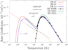 |
Fig. 3 Total Maxwellian-averaged DR and RR ground-state rate coefficients for S+: (a) the solid black curve (DR MM98) shows the previous recommended data of Mazzotta et al. (1998); (b) the solid red and dashed curves represent our total IC DR and RR rate coefficients, respectively; (c) the solid green (DR DD21) and dotted (RR DD21) curves represent the DR and RR rate coefficients of Dufresne et al. (2021). |
4.1 Fe11+
The experimentally derived Maxwellian rate coefficients of Novotnỳ et al. (2012) are compared with our total Fe11+ DR rate coefficients in Fig. 2, along with those of the previous AUTOSTRUCTURE calculations by Badnell (2006b). Our calculations differ somewhat from the previous calculations of Badnell (2006b), as described in Sect. 2. The overall agreement of the experimental measurements by Novotnỳ et al. (2012) (green curve) with both our total IC DR rate coefficients (solid red curve) and with the total IC DR rate coefficients previously calculated by Badnell (2006b) (broken magenta curve) is quite good over the energy range of the measurements. The difference between the present and the previous results is found to be about 35% at 3 × 10⁴ K near the middle of the photoionized plasma zone. In contrast, the difference with the data recommended by Mazzotta et al. (1998) (black curve) only drops to less than a factor of two above 106 K. Our IC RR rate coefficients (short-dashed red curve) are negligible compared to DR at temperatures of most interest. Only below ≈500 K does RR dominate over DR.
It should also be noted that the contribution from the 3 → 4 core excited DR process to our total DR rate coefficients above 5 × 10⁵ K is about 8%. The agreement of the present and the previously calculated IC DR results with the measurements (Novotnỳ et al. 2012) at peak temperature at about 103 K are within 27% and 44%, respectively. These percentages become 50% and 30% at the centre of photoionized plasma zone temperatures, respectively. At temperatures above 5 × 10⁵ K, the present and previously calculated results are indistinguishable, and the agreement between the measurements is within a maximum of 2%.
4.2 S+
In Fig. 3, we compare our LS & IC DR and IC RR rate coefficients for S+ with those from the results of recent calculations reported by Dufresne et al. (2021) also using AUTOSTRUCTURE, along with the recommended DR rate coefficients of Mazzotta et al. (1998). Our IC RR rate coefficients (dashed red curve) are indistinguishable from those of Dufresne et al. (2021) (dashed green curve) below a temperature of 2 × 10⁴ K. The two sets of results start to differ at higher temperatures, those of Dufresne et al. (2021) being 50% higher at 106 K. High-energy photoionization cross sections start to suffer from cancellation error as they become increasing small and correspondingly start to affect the accuracy of the RR rate coefficients at higher temperatures. We in fact show our fitted results, which are constrained to have the correct high-T behaviour.
The agreement between our IC DR rate coefficients (solid red curve) and the DR rate coefficients (solid green curve) of Dufresne et al. (2021) below 2 × 10⁴ K is very good in both shape and size. At higher temperatures, the difference between the two sets of results increases. At the high-temperature peak, those of Dufresne et al. (2021) are a factor of two larger. The magnitude of this high-temperature peak is strongly correlated with the magnitude of the oscillator strengths that we show in Table 4, as was noted previously (Badnell 1991). It should be noted that at this temperature, one is at the extreme end of applicability even to collisional plasma environments.
The DR rate coefficients (solid black curve with small squares) extracted from the recommended fitting set by Mazzotta et al. (1998) agree quite well in both shape and size at temperatures above 2 × 10⁵ K with both our IC and LS DR rates (solid red curve). Our IC DR rate coefficients for S+ display two distinct peaks, one dominating the low-temperature region and one the high-temperature region. The major contribution for the build up of the higher peak comes from the 3p → 3d core-dipole excited Rydberg autoionizing resonances. The lower peak has contributions from the 3 → 3, 3 DR process as well as the low-lying 3p → 3d core-dipole excited Rydberg autoionizing resonances.
Finally, it is worth mentioning some further details about our calculations for S+. According to the NIST database, the 3s23p3 (2D) 3d [3D1,2,3] levels are autoionizing but energetically degenerate with the common energy value of 0.765 Ry. According to our calculations, these levels are also autoionizing with non-degenerate energies of 0.723905, 0.724250, and 0.724661 Ry, respectively. Given the definite uncertainties in these levels, as listed in the NIST table, and the fact that the NIST degenerate energy value is higher than our results, we made small energetic adjustments to relocate level energies in the post-processing step of our rate calculations to centre the 3s23p3 (2D) 3d [3D2] middle level at 0.765 − 0.76145 = 0.00355 above our calculated first ionization threshold of neutral sulphur.
4.3 Remaining ions
Our Maxwellian-averaged LS and IC DR and RR rate coefficients for Cl2+, Ar3+, K4+, Ca5+, Sc6+, and Ti7+ are compared with the DR rate coefficients extracted from the corresponding recommended fitting coefficients of Mazzotta et al. (1998) in Fig. 4, represented by the solid black curve with small squares. Except for Cl2+, DR rates of all other ions in this figure show reasonable agreement in both shape and magnitude with the recommended DR data from Mazzotta et al. (1998) for the electron temperatures above ≈ 3 × 10⁵ K. We should note that the large disagreement seen for Cl2+, even at the high-temperature peak, is not due to any sensitivity in our atomic structure.
The broad two-peak DR structure, one at a low temperature and one at a high temperature, as we have seen for S+, is a common characteristic of these ions, except for K4+, which clearly shows three peaks. The first peak in DR rate coefficients of K4+ indicates the existence of autoionizing resonances very near the first threshold of K3+, in our calculations. It should be noted that the lower two peaks entirely result from the autoionization of the recombined states resulting from the 3 → 3, 3(, n) processes. The 3 → 4, 4(, n) processes start contributing to DR rates beyond approximately 103 K. The relative contribution of these processes to the total DR rates at about 2 × 10⁵ K is found to be less than 1%. We should also note that the larger number of fine structure split levels of the electron configurations describing the target ions gives rise to many more Rydberg series that are part of IC DR calculations, but which are degenerate in the corresponding LS DR calculations. This gives a greater likelihood of there being near-threshold resonances and is the reason why the IC DR rate coefficients are much larger than the corresponding LS ones at lower temperatures.
Figure 5 displays our Maxwellian-averaged LS and IC DR and RR rate coefficients for V8+, Cr9+, Mn10+, Fe11+, Co12+, and Ni13+. For all ions in Fig. 5, the IC DR rate coefficients are higher than the LS ones over the entire temperature range shown. The solid black curves with small squares in different panels of Fig. 5 represent the DR rate coefficients extracted from the corresponding recommended fitting coefficients of Mazzotta et al. (1998), which agree with our results only for temperatures above 106 K, as can be seen from the figures. We should note that there are no low-temperature contributions in any of the Mazzotta et al. (1998) data. This means there are no low-lying resonances in the original calculations on which these data are based – see the beginning of Sect. 4. The large disagreements between the present MCBP DR rates and the rates of Mazzotta et al. (1998) seen in Figs. 4 and 5 at the low temperatures are due to the absence of such low-temperature contributions from their data. The short-dashed red lines in various panels of Figs. 4 and 5 represent our IC RR rate coefficients, which all display expected behaviours as a function of temperature. Results for Zn15+ (not shown) are very similar to those of Cu14+, explicitly plotted in the last panel of Fig. 5. The low-temperature part of the LS DR rate coefficients of these two ions are considerably lower than the corresponding IC ones. We may interprete this behaviour as being due to the presence of strong resonance levels near the first ionization thresholds of Cu13+ and Zn14+ ions. We have not explicitly plotted DR and RR rate coefficients for Kr21+, Mo27+, Xe39+, and W59+ ions – their fitting coefficients are given in Tables 2 and 3.
Oscillator strengths for transitions that dominate the (high-T) DR of S+ and Fe11+.
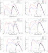 |
Fig. 4 Present Maxwellian-averaged DR and RR rate coefficients for Cl2+–Ti7+ ions: (a) the solid blue and red curves represent our total LS and IC DR results, respectively; (b) the solid black curve (DR MM98) shows the previous recommended data of Mazzotta et al. (1998); (c) the dashed red curve represents the present IC RR results. |
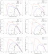 |
Fig. 5 Present Maxwellian-averaged DR and RR rate coefficients for V8+–Cu14+ ions: (a) the solid red and blue curves represent our total IC and LS DR results, respectively; (b) the solid black curve (DR MM98) shows the previous recommended data of Mazzotta et al. (1998); (c) the dashed red curve represents the present IC RR results. |
5 Summary and conclusions
We have performed systematic calculations of the DR and RR rate coefficients for the P-like isoelectronic sequence as part of the assembly of a level-resolved DR and RR database necessary for modelling dynamic finite-density plasmas (Badnell et al. 2003). Calculations were carried out in both multi-configuration LS- and Breit-Pauli intermediate coupling approximations for S+ to Zn15+, as well as Kr21+, Mo27+, Xe39+, and W59+ using non-relativistic (up to Zn) and kappa-averaged relativistic (from Zn) radial orbitals. The DR rate coefficients obtained for Fe11+ are compared with the merged-beam measurements by Novotnỳ et al. (2012). Given the complexity of the problem, the agreement between our results and the measurements is very good at high energies. At low energies, the agreement is only good for broad features with increasing differences in details. The agreement between our IC DR and RR rate coefficients with the recent S+ calculations of Dufresne et al. (2021) is found to be quite good. These are the first systematic DR and RR rate coefficient calculations for the phosphorous-like isoelectronic sequence, the results of which are presented in tables in the form useful for the modellers of both astrophysical and fusion plasmas. The results of our calculations will also be available at OPEN-ADAS4. We have made comparisons, where possible, with the DR rate coefficients extracted from the recommended fitting coefficients by Mazzotta et al. (1998). In all the DR figures, the bars indicating the collisionally and photoionized ionized zones were drawn to facilitate the use of the underline data by the modelers.
The DR and RR rate coefficients are archived in OPEN-ADAS via the ADAS adf09 and adf48 formats, respectively. The literature lacks in both theoretical and experimental results characterizing DR and RR rate coefficients of phosphorous-like ions, which are important for laboratory and astrophysical plasmas. We very much hope our calculations will stimulate further studies in this respect.
Acknowledgements
E.A.B. acknowledges the computational support from TUBITAK ULAKBIM, High Performance and Grid Computing Center (TRUBA resources) and BAPKO of Marmara University. Z.A. thanks to National Energy Research Scientific Computing Center (NERSC) in Oakland, California for computational support and also to Mr. Orkan Akcan for local support. NRB was supported by the UK STFC under grant number ST/V000683/1 with the University of Strathclyde.
References
- Abdel-Naby, S. A., Nikolić, D., Gorczyca, T. W., Korista, K.T., & Badnell, N.R. 2012, A&A, 537, A40 [NASA ADS] [CrossRef] [EDP Sciences] [Google Scholar]
- Altun, Z., Yumak, A., Badnell, N. R., Colgan, J., & Pindzola, M. S. 2004, A&A, 420, 775 [NASA ADS] [CrossRef] [EDP Sciences] [Google Scholar]
- Altun, Z., Yumak, A., Badnell, N. R., Loch, S. D., & Pindzola, M. S. 2006, A&A, 447, 1165 [NASA ADS] [CrossRef] [EDP Sciences] [Google Scholar]
- Altun, Z., Yumak, A., Yavuz, I., et al. 2007, A&A, 474, 1051 [NASA ADS] [CrossRef] [EDP Sciences] [Google Scholar]
- Arnaud, K. A. 1996, in Astronomical Data Analysis Software and Systems V, 101, 17 [Google Scholar]
- Badnell, N. R. 1986, J. Phys. B, 19, 3827 [NASA ADS] [CrossRef] [Google Scholar]
- Badnell, N. R. 1991, ApJ, 379, 356 [NASA ADS] [CrossRef] [Google Scholar]
- Badnell, N. R. 1997, J. Phys. B, 30, 1 [NASA ADS] [CrossRef] [Google Scholar]
- Badnell, N. R. 2006a, A&A, 447, 389 [NASA ADS] [CrossRef] [EDP Sciences] [Google Scholar]
- Badnell, N. R. 2006b, ApJ, 651, L73 [NASA ADS] [CrossRef] [Google Scholar]
- Badnell, N. R. 2006c, J. Phys. B, 39, 4825 [NASA ADS] [CrossRef] [Google Scholar]
- Badnell, N. R. 2006d, ApJS, 167, 334 [Google Scholar]
- Badnell, N. R. 2011, Comput. Phys. Commun., 182, 1528 [NASA ADS] [CrossRef] [Google Scholar]
- Badnell, N. R., & Pindzola, M. S. 1992, Phys. Rev. A, 45, 2820 [CrossRef] [Google Scholar]
- Badnell, N. R., O'Mullane, M.G., Summers, H.P., et al. 2003, A&A, 406, 1151 [NASA ADS] [CrossRef] [EDP Sciences] [Google Scholar]
- Bates, D. R., Kingston, A. E., & McWhirter, R. W. P. 1962, Proc. Roy. Soc. Lond. Ser. A Math. Phys. Sci., 267, 297 [Google Scholar]
- Bautista, M. A., & Badnell, N. R. 2007, A&A, 466, 755 [NASA ADS] [CrossRef] [EDP Sciences] [Google Scholar]
- Behar, E., Jacobs, V. L., Oreg, J., Bar-Shalom, A., & Haan, S. L. 2000, Phys. Rev. A, 62, 030501 [NASA ADS] [CrossRef] [Google Scholar]
- Bryans, P., Badnell, N. R., Gorczyca, T. W., et al. 2006, ApJS, 167, 343 [NASA ADS] [CrossRef] [Google Scholar]
- Bryans, P., Landi, E., & Savin, D. W. 2009, ApJ, 691, 1540 [CrossRef] [Google Scholar]
- Burgess, A. 1964, ApJ, 139, 776 [NASA ADS] [CrossRef] [Google Scholar]
- Burgess, A. 1965, ApJ, 141, 1588 [NASA ADS] [CrossRef] [Google Scholar]
- Burgess, A., & Summers, H. P. 1969, ApJ, 157, 1007 [NASA ADS] [CrossRef] [Google Scholar]
- Burgess, A., Mason, H. E., & Tully, J. A. 1989, A&A, 217, 319 [NASA ADS] [Google Scholar]
- Colgan, J., Pindzola, M. S., Whiteford, A. D., & Badnell, N. R. 2003, A&A, 412, 597 [NASA ADS] [CrossRef] [EDP Sciences] [Google Scholar]
- Colgan, J., Pindzola, M. S., & Badnell, N. R. 2004, A&A, 417, 1183 [NASA ADS] [CrossRef] [EDP Sciences] [Google Scholar]
- Del Zanna, G., & Mason, H. E. 2018, Living Rev. Solar Phys., 15, 1 [Google Scholar]
- Del Zanna, G., Dere, K. P., Young, P. R., & Landi, E. 2021, ApJ, 909, 38 [NASA ADS] [CrossRef] [Google Scholar]
- Dufresne, R. P., Del Zanna, G., & Storey, P. J. 2021, MNRAS, 505, 3968 [NASA ADS] [CrossRef] [Google Scholar]
- Eissner, W., & Nussbaumer, H. 1969, J. Phys. B: At. Mol. Phys., 2, 1028 [NASA ADS] [CrossRef] [Google Scholar]
- Ercolano, B., Young, P. R., Drake, J. J., & Raymond, J. C. 2007, ApJS, 175, 534 [Google Scholar]
- Ferland, G. J., Korista, K. T., Verner, D. A., et al. 1998, PASP, 110, 761 [Google Scholar]
- Fritzsche, S. 2021, A&A, 656, A163 [NASA ADS] [CrossRef] [EDP Sciences] [Google Scholar]
- Froese Fischer, C., Tachiev, G., & Irimia, A. 2006, ADNDT, 92, 607 [CrossRef] [Google Scholar]
- Gabriel, A. H. 1972, MNRAS, 160, 99 [NASA ADS] [Google Scholar]
- Gu, M. F. 2003, ApJ, 589, 1085 [NASA ADS] [CrossRef] [Google Scholar]
- Hahn, Y. 1997, Rep. Progr. Phys., 60, 691 [CrossRef] [Google Scholar]
- Holczer, T., Behar, E., & Arav, N. 2009, ApJ, 708, 981 [Google Scholar]
- Irimia, A., & Froese Fischer, C. 2005, Physica Scripta, 71, 172 [NASA ADS] [CrossRef] [Google Scholar]
- Kaastra, J. S., Mewe, R., & Nieuwenhuijzen, H. 1996, UV and X-ray Spectroscopy of Astrophysical and Laboratory Plasmas, 411 [Google Scholar]
- Kallman, T., & Bautista, M. 2001, ApJS, 133, 221 [Google Scholar]
- Kaur, J., Gorczyca, T. W., & Badnell, N. R. 2018, A&A, 610, A41 [NASA ADS] [CrossRef] [EDP Sciences] [Google Scholar]
- Landini, M., & Fossi, B. C. M. 1991, A&AS, 91, 183 [Google Scholar]
- Lestinsky, M., Lindroth, E., Orlov, D. A., et al. 2008, Phys. Rev. Lett., 100, 033001 [NASA ADS] [CrossRef] [Google Scholar]
- Mattioli, M. 1988, Euratom-CEA Report No., Tech. rep., EUR-CEA-FC-1346 [Google Scholar]
- Mazzotta, P., Mazzitelli, G., Colafrancesco, S., & Vittorio, N. 1998, A&AS, 133, 403 [NASA ADS] [CrossRef] [EDP Sciences] [Google Scholar]
- Mendoza, C., Bautista, M. A., Deprince, J., et al. 2021, Atoms, 9, 12 [CrossRef] [Google Scholar]
- Mewe, R., Kaastra, J. S., & Liedahl, D. A. 1995, Legacy, 6, 16 [Google Scholar]
- Mitnik, D. M., & Badnell, N. R. 2004, A&A, 425, 1153 [NASA ADS] [CrossRef] [EDP Sciences] [Google Scholar]
- Müller, A. 2008, Adv. At. Mol. Opt. Phys., 55, 293 [CrossRef] [Google Scholar]
- Nahar, S. N., & Pradhan, A. K. 1997, ApJS, 111, 339 [NASA ADS] [CrossRef] [Google Scholar]
- Nikolić, D., Gorczyca, T. W., Korista, K. T., & Badnell, N. R. 2010, A&A, 516, A97 [NASA ADS] [CrossRef] [EDP Sciences] [Google Scholar]
- Novotnỳ, O., Badnell, N. R., Bernhardt, D., et al. 2012, ApJ, 753, 57 [CrossRef] [Google Scholar]
- Nussbaumer, H., & Storey, P. J. 1983, in Symposium-International Astronomical Union, 103 (Cambridge University Press), 513 [CrossRef] [Google Scholar]
- Pindzola, M. S., Badnell, N. R., & Griffin, D. C. 1992, Phys. Rev. A, 46, 5725 [NASA ADS] [CrossRef] [Google Scholar]
- Preval, S. P., Badnell, N. R., & O'Mullane, M.G. 2016, Phys. Rev. A, 93, 042703 [CrossRef] [Google Scholar]
- Sako, M., Kahn, S. M., Behar, E., et al. 2001, A&A, 365, L168 [NASA ADS] [CrossRef] [EDP Sciences] [Google Scholar]
- Sako, M., Kahn, S. M., Branduardi-Raymont, G., et al. 2003, ApJ, 596, 114 [NASA ADS] [CrossRef] [Google Scholar]
- Savin, D. W., & Laming, J. M. 2002, ApJ, 566, 1166 [NASA ADS] [CrossRef] [Google Scholar]
- Savin, D. W., Bartsch, T., Chen, M. H., et al. 1997, ApJ, 489, L115 [NASA ADS] [CrossRef] [Google Scholar]
- Schippers, S., Müller, A., Gwinner, G., et al. 2001, ApJ, 555, 1027 [NASA ADS] [CrossRef] [Google Scholar]
- Shull, J. M., & Van Steenberg, M. 1982, ApJS, 48, 95 [NASA ADS] [CrossRef] [Google Scholar]
- Smith, R. K., Brickhouse, N. S., Liedahl, D. A., & Raymond, J. C. 2001, ApJ, 556, L91 [Google Scholar]
- Summers, H. P. 2004, The ADAS User Manual, Version 2.6, http://adas.phys.strath.ac.uk, last accessed on 8 May 2022 [Google Scholar]
- Summers, H. P., Dickson, W. J., O'Mullane, M.G., et al. 2006, Plasma Phys. Controlled Fusion, 48, 263 [NASA ADS] [CrossRef] [Google Scholar]
- Tayal, S. S., & Zatsarinny, O. 2010, ApJS, 188, 32 [NASA ADS] [CrossRef] [Google Scholar]
- Verner, D. A., & Ferland, G. J. 1996, ApJS, 103, 467 [NASA ADS] [CrossRef] [Google Scholar]
- Zatsarinny, O., Gorczyca, T. W., Korista, K. T., Badnell, N. R., & Savin, D. W. 2003, A&A, 412, 587 [NASA ADS] [CrossRef] [EDP Sciences] [Google Scholar]
- Zatsarinny, O., Gorczyca, T. W., Korista, K., Badnell, N. R., & Savin, D. W. 2004a, A&A, 426, 699 [NASA ADS] [CrossRef] [EDP Sciences] [Google Scholar]
- Zatsarinny, O., Gorczyca, T. W., Korista, K. T., Badnell, N. R., & Savin, D. W. 2004b, A&A, 417, 1173 [NASA ADS] [CrossRef] [EDP Sciences] [Google Scholar]
- Zatsarinny, O., Gorczyca, T. W., Korista, K. T., et al. 2005, A&A, 438, 743 [NASA ADS] [CrossRef] [EDP Sciences] [Google Scholar]
- Zatsarinny, O., Gorczyca, T. W., Fu, J., et al. 2006, A&A, 447, 379 [NASA ADS] [CrossRef] [EDP Sciences] [Google Scholar]
apap-network.org. Last accessed on 29 March 2022.
http://amdpp.phys.strath.ac.uk/AUTOS/. Last accessed on 6 April 2022.
https://physics.nist.gov/PhysRefData/ASD/levels_form.html. Last accessed on 18 March 2022.
http://open.adas.ac.uk. Last accessed on 18 March 2022.
All Tables
Oscillator strengths for transitions that dominate the (high-T) DR of S+ and Fe11+.
All Figures
|
Fig. 1 Present IC DR rate coefficients for the ground state of Fe11+, as a function of centre-of-mass collision energy in the range 0 to 70 eV. This energy region is dominated by the ∆n = 0 core dipole-excited resonances; (a) the solid green curve denotes our IC results where energy-averaged DR cross sections (× velocity) have been convoluted with the experimental merged-beam electron energy distribution, characterized by the electron temperatures kBT⟘ = 12.00 meV and kBT = 0.09 meV (and without the field ionization effects); (b) the solid blue curve with dots denotes the measured merged-beam recombination rate coefficient by Novotnỳ et al. (2012); (c) the solid orange curve denotes the previous calculations by Badnell (2006b), as given Fig. 2 of the paper by Novotnỳ et al. (2012); (d) the solid black curve differs from the solid green curve only now that we include field ionization effects; (e) the solid magenta curve represents our IC DR rate coefficients with the convolution describing the electron beam energy spread according to somewhat lower temperatures, kBT⟘ = 1.5 meV and kBT = 0.025 meV. |
| In the text | |
|
Fig. 2 Total Maxwellian-averaged DR and RR ground-state rate coefficients for Fe11+: (a) the solid black curve with small squares (DR MM98) represents the recommended DR rates extracted from the fitted coefficients of Mazzotta et al. (1998); (b) the solid red and blue curves represent our IC and LS DR rates, respectively; (c) the dashed red curve is our IC RR rates; (d) the dash-dotted magenta curve (DR B06) represents the previous AUTOSTRUCTURE calculations of Badnell (2006b); (e) the solid green curve (DR NBB12) with error bars represents the experimental results of Novotnỳ et al. (2012). |
| In the text | |
|
Fig. 3 Total Maxwellian-averaged DR and RR ground-state rate coefficients for S+: (a) the solid black curve (DR MM98) shows the previous recommended data of Mazzotta et al. (1998); (b) the solid red and dashed curves represent our total IC DR and RR rate coefficients, respectively; (c) the solid green (DR DD21) and dotted (RR DD21) curves represent the DR and RR rate coefficients of Dufresne et al. (2021). |
| In the text | |
|
Fig. 4 Present Maxwellian-averaged DR and RR rate coefficients for Cl2+–Ti7+ ions: (a) the solid blue and red curves represent our total LS and IC DR results, respectively; (b) the solid black curve (DR MM98) shows the previous recommended data of Mazzotta et al. (1998); (c) the dashed red curve represents the present IC RR results. |
| In the text | |
|
Fig. 5 Present Maxwellian-averaged DR and RR rate coefficients for V8+–Cu14+ ions: (a) the solid red and blue curves represent our total IC and LS DR results, respectively; (b) the solid black curve (DR MM98) shows the previous recommended data of Mazzotta et al. (1998); (c) the dashed red curve represents the present IC RR results. |
| In the text | |
Current usage metrics show cumulative count of Article Views (full-text article views including HTML views, PDF and ePub downloads, according to the available data) and Abstracts Views on Vision4Press platform.
Data correspond to usage on the plateform after 2015. The current usage metrics is available 48-96 hours after online publication and is updated daily on week days.
Initial download of the metrics may take a while.