| Issue |
A&A
Volume 668, December 2022
|
|
|---|---|---|
| Article Number | A33 | |
| Number of page(s) | 11 | |
| Section | Astrophysical processes | |
| DOI | https://doi.org/10.1051/0004-6361/202243352 | |
| Published online | 29 November 2022 | |
Spectral properties and energy transfer at kinetic scales in collisionless plasma turbulence
1
Department of Mathematics, KU Leuven, Celestijnenlaan 200B, 3001 Leuven, Belgium
e-mail: giuseppe.arro@kuleuven.be
2
Dipartimento di Fisica “E. Fermi”, Universitá di Pisa, Largo Bruno Pontecorvo 3, 56127 Pisa, Italy
Received:
17
February
2022
Accepted:
8
October
2022
Context. Recent satellite observations in the solar wind and in the Earth’s magnetosheath have shown that the turbulent magnetic field spectrum, which is know to steepen around ion scales, has another break at electron scales where it becomes even steeper. The origin of this second spectral break is not yet fully understood, and the shape of the magnetic field spectrum below electron scales is still under debate.
Aims. By means of a fully kinetic simulation of freely decaying plasma turbulence, we study the spectral properties and the energy exchanges characterizing the turbulent cascade in the kinetic range.
Methods. We started by analyzing the magnetic field, electron velocity, and ion velocity spectra at fully developed turbulence. We then investigated the dynamics responsible for the development of the kinetic scale cascade by analyzing the ion and electron filtered energy conversion channels, represented by the electromagnetic work J ⋅ E, pressure–strain interaction −P : ∇ u, and the cross-scale fluxes of electromagnetic (e.m.) energy and fluid flow energy, accounting for the nonlinear scale-to-scale transfer of energy from large to small scales.
Results. We find that the magnetic field spectrum follows the k−α exp(−λ k) law at kinetic scales with α ≃ 2.73 and λ ≃ ρe (where ρe is the electron gyroradius). The same law with α ≃ 0.94 and λ ≃ 0.87ρe is observed in the electron velocity spectrum, but not in the ion velocity spectrum that drops as a steep power law ∼k−3.25 before reaching electron scales. By analyzing the filtered energy conversion channels, we find that electrons play a major role with respect to the ions in driving the magnetic field dynamics at kinetic scales. Our analysis reveals the presence of an indirect electron-driven mechanism that channels the e.m. energy from large to sub-ion scales more efficiently than the direct nonlinear scale-to-scale transfer of e.m. energy. This mechanism consists of three steps. In the first step the e.m. energy is converted into electron fluid flow energy at large scales; in the second step the electron fluid flow energy is nonlinearly transferred toward sub-ion scales; in the final step the electron fluid flow energy is converted back into e.m. energy at sub-ion scales. This electron-driven transfer drives the magnetic field cascade up to fully developed turbulence, after which dissipation becomes dominant and the electrons start to subtract energy from the magnetic field and dissipate it via the pressure–strain interaction at sub-ion scales.
Key words: plasmas / turbulence / solar wind
© G. Arró et al. 2022
 Open Access article, published by EDP Sciences, under the terms of the Creative Commons Attribution License (https://creativecommons.org/licenses/by/4.0), which permits unrestricted use, distribution, and reproduction in any medium, provided the original work is properly cited.
This article is published in open access under the Subscribe-to-Open model. Subscribe to A&A to support open access publication.
1. Introduction
Turbulence in collisionless magnetized plasmas is a process involving the nonlinear transfer of energy across a wide range of scales, extending from large fluid magnetohydrodynamic (MHD) scales, where the energy is typically injected, down to ion and electron kinetic scales, associated with different physical regimes. Such a complex turbulent cascade still lacks a complete theoretical description and plasma turbulence is mainly studied by means of numerical simulations and satellite measurements conducted in the solar wind (SW) and in the Earth’s magnetosphere (Bruno & Carbone 2005; Matthaeus 2021).
The multiscale nature of plasma turbulence is reflected in the shape of the turbulent spectra that exhibit different behaviors in different ranges of scales. Solar wind in situ observations show that the magnetic field spectrum follows a power law at large MHD scales, with a scaling exponent ranging between −3/2 and −5/3 depending on certain conditions, such as the SW speed and the heliocentric distance (Biskamp 2003; Chen et al. 2013, 2020). Similar MHD scale power laws are also observed in the magnetic spectra measured in the Earth’s magnetosheath, although they are usually shallower than k−3/2 in regions close to the bow shock and tend to the Kolmogorov-like ∼k−5/3 spectrum when moving toward the flanks of the magnetopause (Huang et al. 2017; Stawarz et al. 2019). Both SW and magnetosheath measurements show that the magnetic field spectrum breaks and steepens at ion scales. Here a different power law develops, with a scaling exponent that varies between −2 and −4 close to the transition from MHD to sub-ion scales and seems to tend to ∼k−2.8 when approaching electron scales (Alexandrova et al. 2008, 2013; Bourouaine et al. 2012; Bruno et al. 2014; Stawarz et al. 2016; Li et al. 2020). Electron-scale satellite measurements are harder to obtain, but relatively recent observations reveal the presence of a second break and steepening in the magnetic spectra at scales on the order of the electron gyroradius ρe (e.g., Alexandrova et al. 2009, 2012, 2013, 2021; Sahraoui et al. 2009, 2010, 2013; Huang et al. 2014; Chen & Boldyrev 2017; Macek et al. 2018). The shape of the magnetic spectrum at electron scales is still under debate, and different descriptions have been proposed and tested on satellite data under different conditions. Alexandrova et al. (2012) showed that at scales smaller than ion kinetic scales, down to ρe, the magnetic energy spectra measured in the SW can be described by a law of the form ∼k−α exp(−λ k), with a scaling exponent α ∼ 2.8 and a characteristic length λ on the order of ρe. This scaling, dubbed the exp model, has been tested on a large number of magnetic spectra measured at various distances from the Sun, ranging from 0.3 to 1 AU (Alexandrova et al. 2021). The presence of an exponential decay in the magnetic spectrum, which recalls the exponentially decreasing dissipation range of hydrodynamic turbulence (Chen et al. 1993), is thought to indicate the onset of dissipation that may actually take place at electron scales in collisionless plasma turbulence, with ρe playing the role of the dissipation scale (Alexandrova et al. 2013, 2012, 2021). On the other hand, many cases have been reported in which the shape of the magnetic spectrum below electron scales is better represented by a power law. In Sahraoui et al. (2013) and Huang et al. (2014) a double power law model is used to fit a large number of magnetic spectra at kinetic scales in the SW and in the Earth’s magnetosheath, respectively. A scaling consistent with ∼k−2.8 is found above the electron-scale break, while the scaling exponent shows a broad variation at electron scales, with steeper slopes in the case of the magnetosheath with respect to the SW. Because of these variations the authors suggest that the scaling of turbulence may not be universal at electron scales, even though the scale of the spectral break shows a strong correlation with ρe. A power law scaling at electron scales is also found in Chen & Boldyrev (2017), where the authors compare magnetosheath data with a theoretical model based on inertial kinetic Alfvén waves, and find good agreement between the measured scaling exponent and that predicted by the model. However, the shape of the magnetic field spectrum at electron scales has been shown to be influenced by many factors related to instrumental limitations (Sahraoui et al. 2013; Huang et al. 2014) and by the presence of whistler waves superimposed to the underlying turbulence (Matteini et al. 2017; Lacombe et al. 2014; Roberts et al. 2017). Therefore, to date there is no general agreement about the shape of the magnetic spectrum at electron scales.
Spectral breaks have been observed and studied also in numerical simulations of plasma turbulence. The transition from MHD to sub-ion scales has been examined using both hybrid simulations (e.g., Franci et al. 2015, 2016, 2017; Franci et al. 2020; Cerri et al. 2016, 2017, 2018; Cerri & Califano 2017; Servidio et al. 2015) and fully kinetic simulations (e.g., Roytershteyn et al. 2015; Parashar et al. 2018; Grošelj et al. 2018; González et al. 2019; Cerri et al. 2019; Pecora et al. 2019; Rueda et al. 2021; Adhikari et al. 2021). A general agreement with satellite measurements is found at ion scales, with magnetic spectra whose shape is overall consistent with the observed ion-scale power laws. On the other hand, due to computational limitations, electron scales are harder to investigate in simulations as well. Nevertheless, a steepening in the magnetic spectrum at electron scales has been observed and discussed in fully kinetic simulations of turbulence under different conditions. In Camporeale & Burgess (2011), Chang et al. (2011), Gary et al. (2012), Rueda et al. (2021) and Franci et al. (2022) the authors observe a transition from ion to electron scales consistent with a double power law model, while in Roytershteyn et al. (2015) the observed magnetic spectrum is closely approximated by the exp model. Finally, in Parashar et al. (2018) the effects of plasma β (ratio between the total kinetic pressure and the magnetic pressure) on the turbulence are studied and the authors find that the magnetic spectrum steepens at electron scales, with a curvature that increases with increasing β.
Many attempts have been made to model and explain the spectral steepening at ion and electron kinetic scales, often using reduced models based on specific processes such as wave–particle interactions (Schekochihin et al. 2009; Howes et al. 2011; Boldyrev et al. 2013; TenBarge et al. 2013; Schreiner & Saur 2017), instabilities, and magnetic reconnection (Franci et al. 2017; Loureiro & Boldyrev 2017). A complementary approach to studying the turbulent cascade consists in analyzing the channels responsible for the exchanges between different forms of energy and their relative importance at different scales (Yang et al. 2017a,b; Pezzi et al. 2021). This method, largely employed in hydrodynamic turbulence, was recently applied to plasma turbulence and follows directly from the analysis of the equations for the low-pass filtered fluid flow energy  (with s indicating the species) and electromagnetic (e.m.) energy
  (Matthaeus et al. 2020)

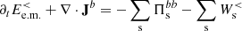
with 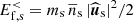 and
and 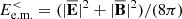 , where ms, ns, and us are respectively the mass, number density, and fluid velocity of particles of species s; E and B are respectively the electric and magnetic fields; the bar
  indicates the low-pass filtering operation, while the hat
  is the density-weighted filtering (i.e.,
  for a generic quantity q, with n being the density) (Favre 1969);
  and Jb are the low-pass filtered fluid flow energy and e.m. energy fluxes respectively, accounting for the spatial transport of energy; and
  and
and  represent the energy flux from large to small scales referring to the fluid flow energy and to the e.m. energy, respectively. The terms actually describing the exchanges between different forms of energy are the low-pass filtered e.m. work done on the particles
  (where Js = qs ns us is the electric current density of species s, with charge qs) and the low-pass filtered pressure–strain interaction
  (where Ps is the pressure tensor of species s and ∇ us = ∂mus, n is the strain tensor, containing the derivatives of us), the latter accounting for the conversion of fluid flow energy into internal (thermal) energy (Del Sarto & Pegoraro 2017). This scale-filtering technique applied to numerical simulations reveals that when the turbulence is fully developed,
  is mainly dominant at scales on the order of a few ion inertial lengths di. On the other hand,
  becomes important at sub-ion scales, thus showing that the e.m. energy is transferred to the fluid flow energy at relatively large scales and finally converted into internal energy at kinetic scales, with
  acting as a bridge between these two conversions taking place at different scales (Yang et al. 2017a, 2018; Matthaeus et al. 2020).
In this work we study the spectral properties of the turbulent cascade at kinetic scales by means of a fully kinetic particle-in-cell (PIC) simulation of freely decaying plasma turbulence and we investigate the development of such spectral features in terms of the filtered energy conversion channels previously described.
2. Simulation setup
The simulation was realized using the energy conserving semi-implicit PIC code ECsim (Lapenta 2017; Markidis & Lapenta 2011). We considered a 2D square periodic domain of size L = 64 di, with 20482 grid points and 5000 particles per cell for each of the two species considered, ions and electrons. The ion-to-electron mass ratio is mi/me = 100, corresponding to an electron inertial length de = 0.1 di. Both species are initialized using a Maxwellian distribution function with uniform density, uniform and isotropic temperature (T⊥ = T∥), and plasma beta equal to βi = 8 for the ions and βe = 2 for the electrons. These parameters were chosen in order to reproduce conditions similar to those met in the Earth’s magnetosheath (see, e.g., Phan et al. 2018; Stawarz et al. 2019; Bandyopadhyay et al. 2020). With these values for βi and βe, the ion and electron gyroradii are equal to 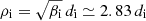 and
and  , respectively, at the beginning of the simulation. A uniform out-of-plane guide field B0 is present and the turbulence is triggered by random phase isotropic magnetic field and velocity perturbations with wavenumber k in the range 1 ≤ k/k0 ≤ 4 (with k0 = 2π/L). In particular, we considered magnetic field fluctuations δB with root mean square amplitude δBrms/B0 ≃ 0.9 and velocity fluctuations δu with δurms/cA ≃ 3.6 (where cA is the Alfvén speed) for both the ions and the electrons. The injection of energy close to ion scales is also justified by the fact that we wanted to reproduce conditions similar to those of the Earth’s magnetosheath, where the correlation length of turbulent fluctuations is typically much smaller than in the SW. The ratio of the plasma frequency to the cyclotron frequency is ωp, i/Ωi = 100 for the ions and ωp, e/Ωe = 10 for the electrons. The time step used to advance the simulation is
  (where Ωe is the electron cyclotron frequency).
3. Results
Figure 1a shows the time evolution of the energy of the system. The total energy Etot is well conserved, with fluctuations that are four orders of magnitude lower than its average value. We see that the e.m. energy Ee.m. increases from the beginning of the simulation, reaches its maximum at about  , and then starts to decrease. The ion fluid flow energy Ef, i monotonically decreases over time, while the initially decreasing electron fluid flow energy Ef, e starts to grow at around
  , reaching its maximum at about
  , after which it starts to decrease again. Both the ion and electron internal energies, Eth, i and Eth, e respectively, monotonically increase over time. Since we trigger the turbulence using high-amplitude velocity fluctuations, we have an excess of Ef, i with respect to Ee.m. at the beginning of the simulation. However, as the system evolves, Ef, i becomes smaller than Ee.m., and when the turbulence is fully developed (
 ) the residual energy σR = (Ef, i − Ee.m.)/(Ef, i + Ee.m.) remains below −0.2, as typically observed both in satellite measurements (Chen et al. 2013) and numerical simulations (Franci et al. 2015).
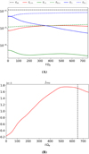 |
Fig. 1. Time evolution of some global quantities characterizing the turbulence. (A) Time evolution of total energy Etot, magnetic energy Ee.m., electron and ion fluid flow energies Ef, e and Ef, i, electron and ion thermal energies Eth, e and Eth, i. (B) Root mean square of the total current Jrms as a function of time. The vertical dashed line indicates the time |

The root mean square (rms) of the total current Jrms is represented in Fig. 1b. At  we see that Jrms has reached and maintains a roughly constant peak value, indicating that the turbulence is fully developed from large to kinetic scales (Mininni & Pouquet 2009; Servidio et al. 2011, 2015). This is seen in Fig. 2 where the shaded contour plots of the modules of the total current J, magnetic field fluctuations δB = |B − B0|, electron velocity ue, and ion velocity ui show a great variety of vortex-like and sheet-like structures consistent with a turbulent flow. We analyzed the turbulent spectra calculated at
  , close to the maximum of Jrms, when the turbulence is fully developed. The magnetic field, electron velocity, and ion velocity spectra PB, Pue, and Pui at
  are shown in Fig. 3, panels A, B, and C, respectively. We analyzed these three spectra since they are representative of the three main forms of energy (i.e., the e.m. energy Ee.m. and the fluid flow energies of electrons and ions, Ef, e and Ef, i, respectively). No small-scale filtering or smoothing has been applied to the spectra. With our simulation setup, the range of scales between the injection scale k di = 4 k0 ≃ 0.39 and k di ≃ 1 is covered only by seven wavenumbers. Nevertheless, we see that all spectra roughly follow a power law that breaks and steepens below k di ≃ 1. In the kinetic range, that is for k di > 1, the magnetic field and electron velocity spectra exhibit a similar behavior, showing a clear negative curvature that becomes more prominent toward k de ≃ 1 and extends into electron scales. On the other hand, no significant curvature is observed for the ion velocity spectrum that does not extend much into electron scales. In analogy with recent studies on satellite data, we fit these spectra in the kinetic range using the exp model proposed by Alexandrova et al. (2012) to describe the SW magnetic field spectrum at sub-ion scales. The range covered by each fit starts at around k di ≃ 1.5, where the spectral break is observed. To decide where to stop the fits, we observe that all spectra become convex at high k beyond electron scales.
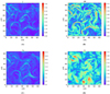 |
Fig. 2. Shaded contour plots of the modules of the (A) total current J, (B) magnetic field fluctuations δB = |B − B0|, (C) electron velocity ue, and (D) ion velocity ui at |

This curvature inversion is most likely caused by the intrinsic numerical noise of PIC codes whose effect is to create small-scale random fluctuations, and thus a bump in the spectra at high k. Hence, each fit stops at the inflection point preceding the convex part of the spectrum.
The results of the fits are shown in Fig. 3 where the fitting curves obtained are plotted on the corresponding spectra in the kinetic range. We see that the exp model k−α exp(−λ k) fits the magnetic field spectrum well at kinetic scales, with a scaling exponent αB ≃ 2.73 and a characteristic length λB ≃ 0.164 ≃ ρe that is equal to the electron gyroradius, whose value is ρe ≃ 0.164 at  in our simulation. Moreover, even the electron velocity spectrum is well described by the exp model at kinetic scales, with a scaling exponent αue ≃ 0.94 and a characteristic length λue = 0.142 ≃ 0.87 ρe that is also on the order of the electron gyroradius ρe. Finally, for the ion velocity spectrum the exp model fit gives a scaling exponent αui = 2.99 and a characteristic length λui = 0.057 ≃ 0.35 ρe, smaller than the electron gyroradius ρe. It is important to note that the characteristic lengths λB and λue of the magnetic field and electron velocity spectra are very similar, which means that their exponential behavior becomes dominant at about the same wavenumbers: kB = 1/λB ≃ 6.1 for the magnetic field and kue = 1/λue ≃ 7 for the electron velocity. On the other hand, the ion velocity spectrum shows a weak exponential behavior in the kinetic range and the power law scaling seems to be dominant. According to the fit, the exponential part of the ion velocity spectrum becomes relevant at kui = 1/λui ≃ 17.5, which falls far beyond ion kinetic scales in the interval where the spectrum is already convex, and thus influenced by the numerical noise. In other words, the exponential behavior introduced by the exp model is not relevant in the range covered by the fit in the case of the ion velocity spectrum. As a comparison, we also fit the ion velocity spectrum with a pure power law model k−β, which gives a scaling exponent βui = 3.25, very close to the value αui = 2.99 obtained with the exp model. The k−3.25 power law is shown in Fig. 3c, compared to the exp model fit. We see that the power law alone is sufficient to describe the behavior of the ion velocity spectrum in the kinetic range and no substantial difference is observed with respect to the exp model. This is confirmed by comparing the goodness of the fits realized with the two models, quantified as the mean square distance between the spectrum and the fitting curve. We find a goodness of Γpower = 7.96 × 10⁻³ for the power law model, very close to the goodness Γexp = 6.01 × 10⁻³ found for the exp model. Thus, we conclude that within the range of kinetic scales covered by our simulation, a power law model is the most appropriate description for the ion velocity spectrum while the magnetic field and electron velocity spectra are well described by the exp model.
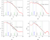 |
Fig. 3. Power spectra at fully developed turbulence. (A) Magnetic field spectrum, (B) electron velocity spectrum, (C) ion velocity spectrum, and (D) ratio of the magnetic to electron velocity spectra at |


The similarities in the shapes of the magnetic field and electron velocity spectra at sub-ion scales suggest that the electrons play a major role with respect to the ions in shaping the magnetic field spectrum at these scales, in particular by contributing to the formation of the electron scale exponential range that is instead absent in the ion velocity spectrum. This is also consistent with the fact that the ions are expected to decouple from the magnetic field dynamics at sub-ion scales (Califano et al. 2020; Sharma Pyakurel et al. 2019). In these conditions, the ion velocity fluctuations become small with respect to the electron velocity fluctuations and if the electron dynamics is mainly incompressible, from the Ampere’s law it follows that ∇ × B ∼ J ∼ ue, which implies k2 PB ∼ Pue. This is indeed observed in our simulation, as shown in Fig. 3d where the ratio of PB to Pue follows the power law ∼k−2 at sub-ion scales, over the whole range where we performed the fits, from k di ≃ 1.5 up to about k di ≃ 20. Hence, it is reasonable to presume that in this range only the incompressible electron dynamics continues to support the magnetic field energy cascade, thus influencing its spectral features.
To investigate the role of the ions and of the electrons in the development of the turbulence from large to sub-ion scales, we study the filtered energy conversion channels introduced in Eqs. (1) and (2). We want to separate the two ranges of scales above and below k di ≃ 1.5, where the spectral breaks are observed. To do so, we consider two groups of filtered energy conversion channels that we indicate as low-pass filtered channels, describing the energy exchanges at scales k di < 1.5, and high-pass filtered channels, accounting for the energy exchanges at scales k di ≥ 1.5. From now on we refer to the scales in the range k di ≥ 1.5 as sub-ion scales, and the scales in the range k di < 1.5 as large scales (with the caveat that our “large” scales should not be interpreted as fluid scales since they are still relatively close to ion scales in our simulation, due to the limited size of the simulation domain). Following Matthaeus et al. (2020), the low-pass filtered e.m. work  and pressure–strain interaction
  are defined as

where the superscript < indicates that these quantities describe the energy exchanges in the range k di < 1.5. The low-pass filter  is defined as in Frisch (1995)
where q(x) is a generic quantity and Q(k) is its Fourier transform. The hat  indicates the density-weighted low-pass filter
  (where n is the density). The high-pass filtered energy conversion channels are obtained by subtracting the low-pass filtered channels from the corresponding unfiltered quantities. Therefore, the high-pass filtered e.m. work
  and pressure–strain interaction
  are defined as


where the superscript > indicates that these quantities describe the energy exchanges in the range k di ≥ 1.5. The pressure–strain interaction can be usefully decomposed as

with ps = tr(Ps)/3, Πs = Ps − ps I and Ds = [(∇ us)+(∇ us)T]/2 − (∇⋅us/3) I, where tr(⋅) is the trace operation, I is the identity matrix, and the superscript T indicates the transpose operation. The first term on the right-hand side of Eq. (8), called the P–θ interaction, describes the increase in internal energy related to isotropic compression and expansion while the second term, called the Pi–D interaction, accounts for the increase in internal energy caused by volume-preserving anisotropic deformations and can be interpreted as a collisionless viscosity (Del Sarto & Pegoraro 2017; Yang et al. 2017a,b; Matthaeus et al. 2020). This decomposition separates the compressible dynamics, described by the P–θ interaction, from the incompressible dynamics, described by the Pi–D interaction. Therefore, we analyzed the low-pass filtered and high-pass filtered P–θ and Pi–D interactions of both ions and electrons to check whether the sub-ion-scale dynamics is actually incompressible, as suggested by the relation between PB and Pue shown in Fig. 3d. The transfer of energy between the two ranges of scales above and below k di ≃ 1.5 is described in terms of the cross-scale energy fluxes  and
and  , defined as (see Matthaeus et al. 2020)

where c is the speed of light. The cross-scale flux  represents the fluid flow energy transferred from the range k di < 1.5 into the range k di ≥ 1.5. Similarly, the cross-scale flux
  accounts for the e.m. energy transferred from the range k di < 1.5 into the range k di ≥ 1.5. Since we are interested in the global energy balance, we analyze the box-averaged energy conversion channels, indicating the average operation with the symbol ⟨ ⋅ ⟩.
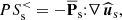
Figure 4 shows the time evolution of the box-averaged low-pass filtered ion and electron energy conversion channels. In Fig. 4a we see that the dominant channels determining the energy balance of the ions at scales k di < 1.5 are the e.m. work  and the pressure–strain interaction
  , while the cross-scale energy fluxes
  and
and  are much smaller in magnitude. The value of
  is negative from the beginning of the simulation and approaches zero after the turbulence is fully developed (
 ), meaning that the ions are giving energy to the e.m. field at scales k di < 1.5. On the other hand,
  is positive during the whole simulation, which means that the ion fluid flow energy is also being converted into internal energy at large scales. The decomposition of
  in Fig. 4b shows that most of the ion heating at large scales results from an incompressible dynamics since the main contribution to
  comes from the Pi–D interaction
  . Differently from the ions, in Fig. 4c we see that in the case of the electrons the cross-scale fluxes
  and
and  are of the same order as
  and
and  at scales k di < 1.5. The value of
  is positive during the whole simulation, meaning that the electrons are taking energy from the e.m. field at large scales;
  and
and  are also positive, which means that the fluid flow energy gained via the e.m. work
  is partially converted into internal energy by the
  interaction, while another consistent fraction is transferred to sub-ion scales by the cross-scale flux of fluid flow energy
  . The electron cross-scale flux of e.m. energy
  is positive from the beginning of the simulations and turns negative at about
  . This means that the electrons are initially supporting the transfer of e.m. energy from large to sub-ion scales, while for
  this flux of energy reverts and the e.m. energy at sub-ion scales is transferred to scales k di < 1.5. The
  decomposition in Fig. 4d shows that for
  the large-scale electron dynamics is mainly compressible since most of the pressure–strain interaction is given by
  . However, for
  the
the  interaction becomes dominant with respect to
  and the electron dynamics becomes mainly incompressible. We note that
  ,
,  ,
,  , and
, and  have a peak at about
  that quickly decreases for
  .
.
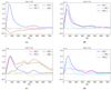 |
Fig. 4. Time evolution of the box-averaged low-pass filtered energy conversion channels of (A) ions and (C) electrons at scales k di < 1.5. Decomposition of the low-pass filtered pressure–strain interaction for (B) ions and (D) electrons. The horizontal black dotted line is centered at zero. |
The presence of this peak is caused by the strong compression and deformation the initial high-amplitude magnetic and velocity fluctuations undergo at the beginning of the simulation. The initial violent dynamics acts as a driver for the formation of current-sheet structures, but as soon as they start to form the peaks quickly settle down.
Figure 5 shows the time evolution of the box-averaged high-pass filtered ion and electron energy conversion channels. In Fig. 5a we see that the main source of energy for the ions at k di ≥ 1.5 is the e.m. work  , which remains positive during the whole simulation. This means that the ions are constantly taking energy from the e.m. field at sub-ion scales. Part of this energy is converted into internal energy via the pressure–strain interaction
  , which is also positive during the whole simulation. Only a very small fraction of the large-scale ion fluid flow energy is transferred to k di ≥ 1.5, as shown by the cross-scale flux
  , which stays negative during the first half of the simulations and turns slightly positive only at about
  . The contribution of the ions to the transport of e.m. energy from large scales to k di ≥ 1.5 is also weak. The cross-scale flux
  initially fluctuates around zero, indicating the absence of a precise direction for the flow of energy between large and sub-ion scales, and finally becomes slightly positive at about
  . The
. The  decomposition in Fig. 5b shows that up to about
  , the main contribution to the pressure–strain interaction comes from
  while only at later times does
  become dominant. For the electrons, the main source of energy at k di ≥ 1.5 is the cross-scale flux of fluid flow energy
  , which remains positive throughout the simulation. The pressure–strain interaction
  is also positive and rapidly grows in time, reaching a roughly constant value at about
  . The e.m. work
  is negative from the beginning of the simulation and changes sign at about
  , after which it remains positive. This change of sign can be understood by comparing
  with
with  and
and  . Among these three channels,
  is the largest one up to
  , and it is the only term providing energy to the electrons at sub-ion scales. On the other hand,
  is positive and
  is negative for
  , which means that the energy delivered by
  is converted both into internal and e.m. energy by
  and
and  , respectively. However, around
  we see that
  becomes larger than
  . This implies that dissipation at sub-ion scales becomes more efficient than the transfer of energy coming from large scales since
  starts to convert more fluid flow energy into internal energy than the amount provided by
  . At this point the electrons are losing fluid flow energy, and to compensate for this loss they start to take energy back from the e.m. field, causing
  to become positive. Therefore, it is possible to distinguish two phases in the evolution of the electrons at sub-ion scales: a first phase for
  , during which the electron dynamics is driven by the cross-scale flux of energy
  , and a second phase for
  , dominated by the pressure–strain interaction
  that takes over in guiding the electron dynamics. Finally, the pressure–strain decomposition in Fig. 5d shows that
  is almost entirely determined by the
  , with a very small negative contribution coming from
  , indicating a weak expansion. This means that the electron dynamics at k di ≥ 1.5 is basically incompressible, which is consistent with the spectral features of the ratio PB/Pue in Fig. 3d.
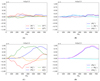 |
Fig. 5. Time evolution of the box-averaged high-pass filtered energy conversion channels of (A) ions and (C) electrons at scales k di ≥ 1.5. Decomposition of the high-pass filtered pressure–strain interaction for (B) ions and (D) electrons. The horizontal black dotted line is centered at zero. |
By comparing the low-pass and the high-pass filtered energy conversion channels, we can finally get an overview of the global energy balance to understand how the e.m. energy is transferred from large scales to sub-ion scales in our simulation. Figure 6 shows a diagram with all the different forms of energy at k di < 1.5 and k di ≥ 1.5 (identified by the superscripts < and >, respectively), together with the energy conversion channels linking them (indicated by the arrows). From this diagram it is possible to identify two paths that the e.m. energy can follow in order to be transferred from k di < 1.5 to k di ≥ 1.5. The first path is the direct scale-to-scale transfer mediated by the total cross-scale flux of e.m. energy, indicated by  , which directly converts
  into
into  . As discussed above, the cross-scale transfer of e.m. energy is not particularly efficient and does not have a preferred direction (its sign changes over time). The flux
  associated with the ions becomes positive only during the second half of the simulation, and its contribution to the energy balance is weak, as seen in Fig. 5a. On the other hand, the flux
  associated with the electrons is positive during the first half of the simulation, but then it turns negative, meaning that the e.m. energy is actually flowing toward large scales though this channel, as seen in Fig. 5c. Therefore,
  is not the main channel responsible for the transfer of e.m. energy from large to sub-ion scales. The second path able to connect
  to
to  involves an indirect transfer of energy driven by the electrons and articulated in three steps. In the first step the e.m. energy
  is converted into the fluid flow energy
  via the e.m. work
  at scales k di < 1.5. In the second step
  is transferred to
  at sub-ion scales via the cross-scale flux
  . In the last step the fluid flow energy
  is finally converted into the e.m. energy
  via the e.m. work
  at scales k di ≥ 1.5. From Figs. 4c and 5c we see that
  ,
,  , and
, and  transfer far more energy than
  , meaning that this second path is the most efficient in transporting the e.m. energy from large to sub-ion scales. As previously discussed, we specify that the second path is accessible only for
  since the sign of
  depends on the relative strength of the cross-scale flux
  with respect to the pressure–strain interaction
  . In particular, this mechanism ceases to act when
  exceeds
  at
at  . At that point
  changes sign and
  starts to be transferred back to
  , and is in turn converted into
  , and thus dissipated. The transition from the
  -dominated phase to the
  -dominated phase is highlighted in Fig. 6 by the presence of the two arrows associated with
  (the orange one refers to
  ; the purple one refers to
  ). We finally observe that, differently from the electrons, the ions do not participate in the transfer of e.m. energy from large to sub-ion scales. On the contrary, since the cross-scale flux
  is weak,
  represents the main source of energy for the ions at sub-ion scales from which they draw upon via
  . In other words, this analysis shows that the development of the e.m. field dynamics at sub-ion scales is indeed guided mainly by the electrons that support the transfer of e.m. energy from large to sub-ion scales up to
  , when the system has reached a fully developed turbulent state.
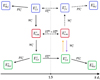 |
Fig. 6. Diagram of the global energy balance between large and sub-ion scales in our simulation. The superscripts < and > indicate quantities at scales k di < 1.5 and k di ≥ 1.5 respectively. The arrows indicate the direction in which the energy is transferred by the corresponding channels (the double arrows indicate no preferred direction). Solid arrows indicate strong channels while weak channels are represented by dashed arrows. The two colors used for |


4. Discussion and conclusions
In this work we used a fully kinetic energy conserving PIC simulation of 2D freely decaying plasma turbulence to study the spectral properties and the energy exchanges characterizing the turbulence at sub-ion scales.
We found that the magnetic field spectrum is accurately described by the exp model k−α exp(−λ k) at sub-ion scales, with a scaling exponent αB ≃ 2.73 and a characteristic length λB ≃ ρe, on the order of the electron gyroradius. To our knowledge, the exp model has been tested on SW data but not in the magnetosheath, whose conditions are closer to those of our simulation. Therefore, we do not have a direct comparison with observations at the moment. Nonetheless, we have found that the functional form proposed by Alexandrova et al. (2012) also works for the magnetic field spectrum produced by our simulation, with parameters consistent with SW observations in the sense that we obtained a scaling exponent close to the SW value −2.8 and a characteristic length associated with the exponential range on the order of the electron gyroradius ρe, even though the actual value of ρe is different in the SW with respect to our simulation since it depends on the electron plasma beta and on other parameters. A few remarks regarding the range over which the fit was performed are needed. Typically, SW observations show that in correspondence with the ion-scale spectral break the slope of the magnetic spectrum varies between −2 and −4, reaching a roughly universal −2.8 spectral index at smaller scales. In the works of Alexandrova et al. (2012, 2021) the exp model is used to fit the magnetic spectrum over a range that starts below the ion scale spectral break, where the ∼k−2.8 scaling is observed, and goes up to electron scales. However, in our simulation the exp model works even if we start the fit directly in correspondence of the spectral break at ion scales. A possible explanation for this difference with respect to SW observations is that the variability in the slope of the SW magnetic spectrum around the ion scale spectral break seems to be induced by instabilities that inject energy around k di ≃ 1 (Alexandrova et al. 2013). These instabilities are triggered by temperature anisotropies generated by the SW expansion (Bale et al. 2009; Alexandrova et al. 2013), an effect that is not present in our simulation, and may thus explain the discrepancy. Another factor influencing the shape of the magnetic spectrum at ion scales is the ion plasma beta βi. In the study of Franci et al. (2016) conducted using hybrid simulations, it is shown that the magnetic field spectrum at sub-ion scales becomes shallower as βi increases, reaching the ∼k−2.8 power law already around k di ≃ 1 (where the spectral break is observed) when βi > 1. This represents another possible reason why in our case the exp models works already from the spectral break downward and with a scaling exponent close to −2.8. The reduced mass ratio mi/me = 100 we used is also another parameter influencing the properties of the spectra. Using a reduced mass ratio implies that the range between ion and electron scales (where the k−2.8 scaling is expected) becomes narrower (but still reasonably separated) and thus electron kinetic effects become relevant at scales larger than in a real plasma. Therefore, to finally confirm our finding, simulations with a more realistic mass ratio are needed in order to properly separate ion and electron scales. However, such simulations have a computational cost that makes them very challenging nowadays, so the mass ratio we used is at the moment a reasonable compromise, and we speculate that if the exp models is universal, a realistic mass ratio would imply a shift of the exponential range toward larger wavenumbers (since a higher mass ratio implies a smaller ρe). Another important point to discuss is the comparison of our results with observational studies supporting the idea of the double power law, in contrast to the exp model. In particular, in Chen & Boldyrev (2017) the magnetic field spectrum measured in the magnetosheath is shown to be consistent with a double power law around electron scales. The authors propose a theoretical model based on inertial kinetic Alfvén waves to explain the steepening observed for k de ≥ 1. This model assumes that βe ≪ βi ≃ 1 (from which it follows that effects related to the electron pressure are weak), and predicts a scale for the spectral break corresponding to 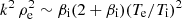 (where Te and Ti are the electron and ion temperatures). In our simulation these conditions on the ion and electron plasma betas are not satisfied since both βi and βe are larger than 1 and the electron pressure plays a key role in the dynamics of the system at sub-ion scales (as discussed in the analysis of the filtered energy conversion channels). Moreover, the model would predict a spectral break at scales k ρe ∼ 2.85 in our simulation (at
  ), corresponding to k di ∼ 17.4, laying inside the exponential range. Therefore, the model proposed in Chen & Boldyrev (2017) is not suited to describe our results. Nonetheless, this comparison shows that the features of the magnetic field spectrum around electron scales may depend on the balance between inertial and kinetic effects of the electrons (i.e., on the value of βe). We speculate that for low βe (as in the observations reported by Chen & Boldyrev 2017) electron inertial effects may cause the development of a power law around k de ≃ 1, while for high βe (as in our simulation) electron kinetic effects may generate an exponential decay around k ρe ≃ 1. However, this point cannot be properly assessed with a single simulation, and a parametric study with respect to βe is needed.
Furthermore, we found that the exp model represents a good description also for the electron velocity spectrum at sub-ion scales, with a scaling exponent αue ≃ 0.94 and a characteristic length λue ≃ 0.87 ρe, very close to the scale λB ≃ ρe found for the magnetic field spectrum. On the other hand, no exponential range was observed in the ion velocity spectrum that does not extend much into electron scales and drops as a steep power law ∼k−3.25 at sub-ion scales. This scaling is remarkably consistent with SW observations reported in Šafránková et al. (2016), where an average spectral index between −3.2 and −3.3 is found for the ion velocity spectrum when 3 ≲ βi ≲ 16 (as in our case where βi = 8 at the beginning of the simulation and increases to βi ≃ 14 at  , due to the ion heating).
We investigated the dynamics responsible for the development of the turbulence from large to sub-ion scales by analyzing the filtered ion and electron energy conversion channels. Our analysis outlines the major role played by the electrons with respect to the ions in driving the magnetic field dynamics at sub-ion scales. We have shown that in our simulation there are two possible channels accounting for the transfer of e.m. energy from large to sub-ion scales: a direct scale-to-scale transfer described by the cross-scale flux of e.m. energy  , and an indirect transfer lead by the electrons that first subtract energy from the e.m. field at large scales (converting it into electron fluid flow energy), then transfer it to sub-ion scales and finally give it back to the e.m. field (see Fig. 6). The latter electron-driven mechanism is far more efficient than the direct scale-to-scale transfer in channelling the e.m. energy from large to sub-ion scales. On the other hand, the ions do not contribute to the transport of e.m. energy to small scales, and we observe only a weak conversion of e.m. energy into ion fluid flow energy at sub-ion scales, which possibly explains why the ion velocity spectrum quickly drops at kinetic scales (consistently with the fact that ions are expected to decouple from the magnetic field at those scales). Therefore, the e.m. field dynamics at kinetic scales is mainly supported by the electrons, and this may explain the similarities in the magnetic field and electron velocity spectra, in particular the presence of an electron scale exponential range that is instead absent in the ion velocity spectrum. We also observed that the electron-driven transfer of e.m. energy acts from the beginning of the simulations and stops at fully developed turbulence when the electron heating becomes more efficient than the cross-scale flux of fluid flow energy coming from large scales. At that point the electrons also start to take energy from the e.m. field and eventually convert it into internal energy. The pressure–strain decomposition shows that this sub-ion-scale electron heating is basically incompressible since it is almost entirely determined by the Pi–D interaction (see Fig. 5d). This transition to a dissipative regime at fully developed turbulence is most likely caused by the lack of a large-scale forcing that maintains the turbulent cascade (i.e., we are dealing with freely decaying turbulence). This implies that there is no large-scale source replacing the energy that is being dissipated at small scales, so once most of the large-scale energy has reached kinetic scales, the transfer of energy to sub-ion scales becomes less efficient than dissipation and we observe the aforementioned transition to a dissipative dynamics. Another point that needs to be discussed is the role of the ions at large scales. In Fig. 4a we saw that the ions lose energy at k di < 1.5 throughout the simulation, both via the pressure–strain interaction and the e.m. work. This behavior could depend on the fact that, with our initialization, most of the initial energy is contained in the ion fluid flow energy that is higher than both the e.m. energy and the electron fluid flow energy (as seen in Fig. 1a). As a consequence, the system may tend to reduce this energy gap by converting the ion fluid flow energy into e.m. energy and ion internal energy. Therefore, we do not claim that the global energy balance observed in our simulation is general and universal because it may depend on various factors such as the way the turbulence is initialized at large scales and the strength of dissipation, determined by the plasma beta, where a higher plasma beta implies a stronger pressure–strain interaction and thus more efficient dissipation, as discussed in Parashar et al. (2018), among others. However, a parametric study with respect to the level of initial fluctuations and the ion and electron plasma betas is beyond the scope of the present paper and will be discussed in future works. Nonetheless, the analysis performed on our simulation shows that the filtered energy conversion channels are indeed a very useful and powerful tool to describe and study the turbulent energy cascade since they allow us to accurately track the path that the energy follows in its way from large to small scales. Finally, another limitation of our work that is worth mentioning is represented by the limited box size and the 2D geometry of our simulation. Additional studies with larger and possibly 3D simulation domains will be needed in order to have results that are finally comparable with satellite observation.
Acknowledgments
This work has received funding from the KULeuven Bijzonder Onderzoeksfonds (BOF) under the C1 project TRACESpace, from the European Union’s Horizon 2020 research and innovation program under grant agreement No. 776262 (AIDA). Computing has been provided by the Flemish Supercomputing Center (VSC) and by the PRACE Tier-0 program. Numerical simulations have been performed on SuperMUC-NG, hosted by the Leibniz Supercomputing Centre (Germany), under the PRACE project. The simulation data-set (KUL_MSH) used in this work is available at Cineca on the AIDA-DB database. In order to access the meta-information and the link to the raw simulation data see the tutorial at http://aida-space.eu/AIDAdb-iRODS.
References
- Adhikari, S., Parashar, T. N., Shay, M. A., et al. 2021, Phys. Rev. E, 104, 065206 [NASA ADS] [CrossRef] [Google Scholar]
- Alexandrova, O., Carbone, V., Veltri, P., & Sorriso-Valvo, L. 2008, ApJ, 674, 1153 [NASA ADS] [CrossRef] [Google Scholar]
- Alexandrova, O., Saur, J., Lacombe, C., et al. 2009, Phys. Rev. Lett., 103 [CrossRef] [Google Scholar]
- Alexandrova, O., Lacombe, C., Mangeney, A., Grappin, R., & Maksimovic, M. 2012, ApJ, 760 [Google Scholar]
- Alexandrova, O., Chen, C., Sorriso-Valvo, L., Horbury, T., & Bale, S. 2013, Space Sci. Rev., 178 [Google Scholar]
- Alexandrova, O., Jagarlamudi, V. K., Hellinger, P., et al. 2021, Phys. Rev. E, 103, 063202 [NASA ADS] [CrossRef] [Google Scholar]
- Bale, S., Kasper, J., Howes, G., et al. 2009, Phys. Rev. Lett., 103, 211101 [Google Scholar]
- Bandyopadhyay, R., Sorriso-Valvo, L., Chasapis, A., et al. 2020, Phys. Rev. Lett., 124, 225101 [CrossRef] [Google Scholar]
- Biskamp, D. 2003, Magnetohydrodynamic Turbulence (Cambridge: Cambridge University Press) [Google Scholar]
- Boldyrev, S., Horaites, K., Xia, Q., & Perez, J. C. 2013, ApJ, 777, 41 [NASA ADS] [CrossRef] [Google Scholar]
- Bourouaine, S., Marsch, E., Alexandrova, O., & Maksimovic, M. 2012, ApJ, 749 [Google Scholar]
- Bruno, R., & Carbone, V. 2005, Liv. Rev. Sol. Phys., 2, 4 [Google Scholar]
- Bruno, R., Trenchi, L., & Telloni, D. 2014, ApJ, 793, L15 [NASA ADS] [CrossRef] [Google Scholar]
- Califano, F., Cerri, S. S., Faganello, M., et al. 2020, Front. Phys., 8, 317 [NASA ADS] [CrossRef] [Google Scholar]
- Camporeale, E., & Burgess, D. 2011, ApJ, 730, 114 [NASA ADS] [CrossRef] [Google Scholar]
- Cerri, S. S., & Califano, F. 2017, New J. Phys., 19, 025007 [NASA ADS] [CrossRef] [Google Scholar]
- Cerri, S. S., Califano, F., Jenko, F., Told, D., & Rincon, F. 2016, ApJ, 822, L12 [NASA ADS] [CrossRef] [Google Scholar]
- Cerri, S. S., Servidio, S., & Califano, F. 2017, ApJ, 846, L18 [NASA ADS] [CrossRef] [Google Scholar]
- Cerri, S., Kunz, M. W., & Califano, F. 2018, ApJ, 856, L13 [CrossRef] [Google Scholar]
- Cerri, S. S., Grošelj, D., & Franci, L. 2019, Front. Astron. Space Sci., 64 [Google Scholar]
- Chang, O., Peter Gary, S., & Wang, J. 2011, Geophys. Res. Lett., 38 [Google Scholar]
- Chen, C. H., & Boldyrev, S. 2017, ApJ, 842, 122 [NASA ADS] [CrossRef] [Google Scholar]
- Chen, S., Doolen, G., Herring, J. R., et al. 1993, Phys. Rev. Lett., 70, 3051 [NASA ADS] [CrossRef] [Google Scholar]
- Chen, C., Bale, S., Salem, C., & Maruca, B. 2013, ApJ, 770, 125 [Google Scholar]
- Chen, C., Bale, S., Bonnell, J., et al. 2020, ApJS, 246, 53 [Google Scholar]
- Del Sarto, D., & Pegoraro, F. 2017, MNRAS, 475, 181 [Google Scholar]
- Favre, A. 1969, Problems of Hydrodynamics and Continuum Mechanics, 231 [Google Scholar]
- Franci, L., Landi, S., Matteini, L., Verdini, A., & Hellinger, P. 2015, ApJ, 812, 21 [NASA ADS] [CrossRef] [Google Scholar]
- Franci, L., Landi, S., Matteini, L., Verdini, A., & Hellinger, P. 2016, ApJ, 833 [Google Scholar]
- Franci, L., Cerri, S. S., Califano, F., et al. 2017, ApJ, 850 [Google Scholar]
- Franci, L., Stawarz, J. E., Papini, E., et al. 2020, ApJ, 898, 175 [NASA ADS] [CrossRef] [Google Scholar]
- Franci, L., Papini, E., Micera, A., et al. 2022, ApJ, 936, 27 [NASA ADS] [CrossRef] [Google Scholar]
- Frisch, U. 1995, Turbulence: The Legacy of AN Kolmogorov (Cambridge: Cambridge University Press) [CrossRef] [Google Scholar]
- Gary, S. P., Chang, O., & Wang, J. 2012, ApJ, 755, 142 [NASA ADS] [CrossRef] [Google Scholar]
- González, C., Parashar, T., Gomez, D., Matthaeus, W., & Dmitruk, P. 2019, Phys. Plasmas, 26 [Google Scholar]
- Grošelj, D., Mallet, A., Loureiro, N. F., & Jenko, F. 2018, Phys. Rev. Lett., 120, 105101 [CrossRef] [Google Scholar]
- Howes, G. G., TenBarge, J. M., & Dorland, W. 2011, Phys. Plasmas, 18, 102305 [NASA ADS] [CrossRef] [Google Scholar]
- Huang, S., Sahraoui, F., Deng, X., et al. 2014, ApJ, 789, L28 [NASA ADS] [CrossRef] [Google Scholar]
- Huang, S., Hadid, L., Sahraoui, F., Yuan, Z., & Deng, X. 2017, ApJ, 836, L10 [NASA ADS] [CrossRef] [Google Scholar]
- Lacombe, C., Alexandrova, O., Matteini, L., et al. 2014, ApJ, 796, 5 [Google Scholar]
- Lapenta, G. 2017, J. Comput. Phys., 334, 349 [NASA ADS] [CrossRef] [Google Scholar]
- Li, H., Jiang, W., Wang, C., et al. 2020, ApJ, 898, L43 [NASA ADS] [CrossRef] [Google Scholar]
- Loureiro, N. F., & Boldyrev, S. 2017, ApJ, 850, 182 [NASA ADS] [CrossRef] [Google Scholar]
- Macek, W., Krasińska, A., Silveira, M., et al. 2018, ApJ, 864, L29 [NASA ADS] [CrossRef] [Google Scholar]
- Markidis, S., & Lapenta, G. 2011, J. Comput. Phys., 230, 7037 [NASA ADS] [CrossRef] [Google Scholar]
- Matteini, L., Alexandrova, O., Chen, C., & Lacombe, C. 2017, MNRAS, 466, 945 [NASA ADS] [CrossRef] [Google Scholar]
- Matthaeus, W. 2021, Phys. Plasmas, 28, 032306 [NASA ADS] [CrossRef] [Google Scholar]
- Matthaeus, W. H., Yang, Y., Wan, M., et al. 2020, ApJ, 891, 101 [NASA ADS] [CrossRef] [Google Scholar]
- Mininni, P. D., & Pouquet, A. 2009, Phys. Rev. E, 80, 025401 [CrossRef] [PubMed] [Google Scholar]
- Parashar, T. N., Matthaeus, W. H., & Shay, M. A. 2018, ApJ, 864, L21 [NASA ADS] [CrossRef] [Google Scholar]
- Pecora, F., Pucci, F., Lapenta, G., Burgess, D., & Servidio, S. 2019, Sol. Phys., 294, 1 [NASA ADS] [CrossRef] [Google Scholar]
- Pezzi, O., Liang, H., Juno, J. L., et al. 2021, MNRAS, 505, 4857 [NASA ADS] [CrossRef] [Google Scholar]
- Phan, T., Eastwood, J., Shay, M., et al. 2018, Nature, 557 [Google Scholar]
- Roberts, O. W., Alexandrova, O., Kajdič, P., et al. 2017, ApJ, 850, 120 [NASA ADS] [CrossRef] [Google Scholar]
- Roytershteyn, V., Karimabadi, H., & Roberts, A. 2015, Philos. Trans. R. Soc. A, 373, 20140151 [NASA ADS] [CrossRef] [Google Scholar]
- Rueda, J. A. A., Verscharen, D., Wicks, R. T., et al. 2021, J. Plasma Phys., 87 [Google Scholar]
- Šafránková, J., Němeček, Z., Němec, F., et al. 2016, ApJ, 825, 121 [CrossRef] [Google Scholar]
- Sahraoui, F., Goldstein, M. L., Robert, P., & Khotyaintsev, Y. V. 2009, Phys. Rev. Lett., 102, 131101 [CrossRef] [Google Scholar]
- Sahraoui, F., Goldstein, M. L., Belmont, G., Canu, P., & Rezeau, L. 2010, Phys. Rev. Lett., 105, 231102 [NASA ADS] [CrossRef] [Google Scholar]
- Sahraoui, F., Huang, S., Belmont, G., et al. 2013, ApJ, 777, 15 [NASA ADS] [CrossRef] [Google Scholar]
- Schekochihin, A. A., Cowley, S. C., Dorland, W., et al. 2009, ApJS, 182, 310 [NASA ADS] [CrossRef] [Google Scholar]
- Schreiner, A., & Saur, J. 2017, ApJ, 835, 133 [NASA ADS] [CrossRef] [Google Scholar]
- Servidio, S., Dmitruk, P., Greco, A., et al. 2011, Nonlin. Proces. Geophys., 18, 675 [NASA ADS] [CrossRef] [Google Scholar]
- Servidio, S., Valentini, F., Perrone, D., et al. 2015, J. Plasma Phys., 81, 325810107 [CrossRef] [Google Scholar]
- Sharma Pyakurel, P., Shay, M. A., Phan, T. D., et al. 2019, Phys. Plasmas, 26 [Google Scholar]
- Stawarz, J., Eriksson, S., Wilder, F., et al. 2016, J. Geophys. Res. Space Phys., 121, 11 [Google Scholar]
- Stawarz, J. E., Eastwood, J. P., Phan, T. D., et al. 2019, ApJ, 877, L37 [NASA ADS] [CrossRef] [Google Scholar]
- TenBarge, J. M., Howes, G. G., & Dorland, W. 2013, ApJ, 774, 139 [NASA ADS] [CrossRef] [Google Scholar]
- Yang, Y., Matthaeus, W. H., Parashar, T. N., et al. 2017a, Phys. Plasmas, 24, 072306 [NASA ADS] [CrossRef] [Google Scholar]
- Yang, Y., Matthaeus, W. H., Parashar, T. N., et al. 2017b, Phys. Rev. E, 95, 061201 [NASA ADS] [CrossRef] [Google Scholar]
- Yang, Y., Wan, M., Matthaeus, W. H., et al. 2018, MNRAS, 482, 4933 [Google Scholar]
All Figures
|
Fig. 1. Time evolution of some global quantities characterizing the turbulence. (A) Time evolution of total energy Etot, magnetic energy Ee.m., electron and ion fluid flow energies Ef, e and Ef, i, electron and ion thermal energies Eth, e and Eth, i. (B) Root mean square of the total current Jrms as a function of time. The vertical dashed line indicates the time |
| In the text | |
|
Fig. 2. Shaded contour plots of the modules of the (A) total current J, (B) magnetic field fluctuations δB = |B − B0|, (C) electron velocity ue, and (D) ion velocity ui at |
| In the text | |
|
Fig. 3. Power spectra at fully developed turbulence. (A) Magnetic field spectrum, (B) electron velocity spectrum, (C) ion velocity spectrum, and (D) ratio of the magnetic to electron velocity spectra at |
| In the text | |
|
Fig. 4. Time evolution of the box-averaged low-pass filtered energy conversion channels of (A) ions and (C) electrons at scales k di < 1.5. Decomposition of the low-pass filtered pressure–strain interaction for (B) ions and (D) electrons. The horizontal black dotted line is centered at zero. |
| In the text | |
|
Fig. 5. Time evolution of the box-averaged high-pass filtered energy conversion channels of (A) ions and (C) electrons at scales k di ≥ 1.5. Decomposition of the high-pass filtered pressure–strain interaction for (B) ions and (D) electrons. The horizontal black dotted line is centered at zero. |
| In the text | |
|
Fig. 6. Diagram of the global energy balance between large and sub-ion scales in our simulation. The superscripts < and > indicate quantities at scales k di < 1.5 and k di ≥ 1.5 respectively. The arrows indicate the direction in which the energy is transferred by the corresponding channels (the double arrows indicate no preferred direction). Solid arrows indicate strong channels while weak channels are represented by dashed arrows. The two colors used for |
| In the text | |
Current usage metrics show cumulative count of Article Views (full-text article views including HTML views, PDF and ePub downloads, according to the available data) and Abstracts Views on Vision4Press platform.
Data correspond to usage on the plateform after 2015. The current usage metrics is available 48-96 hours after online publication and is updated daily on week days.
Initial download of the metrics may take a while.