| Issue |
A&A
Volume 667, November 2022
|
|
|---|---|---|
| Article Number | A163 | |
| Number of page(s) | 13 | |
| Section | Galactic structure, stellar clusters and populations | |
| DOI | https://doi.org/10.1051/0004-6361/202244709 | |
| Published online | 23 November 2022 | |
The star formation history of Upper Scorpius and Ophiuchus
A 7D picture: positions, kinematics, and dynamical traceback ages⋆,⋆⋆
1
University of Vienna, Department of Astrophysics, Türkenschanzstraße 17, 1180 Wien, Austria
e-mail: This email address is being protected from spambots. You need JavaScript enabled to view it.
2
Núcleo de Astrofísica Teórica, Universidade Cidade de São Paulo, R. Galvão Bueno 868, Liberdade, 01506-000 São Paulo, SP, Brazil
3
Departamento de Inteligencia Artificial, Universidad Nacional de Educación a Distancia (UNED), c/Juan del Rosal 16, 28040 Madrid, Spain
4
Laboratoire d’astrophysique de Bordeaux, Univ. Bordeaux, CNRS, B18N, allée Geoffroy Saint-Hilaire, 33615 Pessac, France
5
Centro de Astrobiología (CAB), CSIC-INTA, ESAC Campus, Camino Bajo del Castillo s/n, 28692 Villanueva de la Cañada, Madrid, Spain
Received:
4
August
2022
Accepted:
23
September
2022
Abstract
Context. Understanding how star formation begins and propagates through molecular clouds is a fundamental but still open question. One major difficulty in addressing this question is the lack of precise 3D kinematics and age information for young stellar populations. Thanks to astrometry provided by Gaia, large spectroscopic surveys, and improved age-dating methods, this picture is changing.
Aims. We aim to study spatial and kinematic substructures of the region encompassed by the Upper Scorpius and Ophiuchus star forming regions. We want to determine dynamical traceback ages and study the star formation history (SFH) of the complex.
Methods. We combined our spectroscopic observations with spectra in public archives and large radial velocity surveys to obtain a precise radial velocity sample to complement the Gaia astrometry. We used a Gaussian Mixture Model to identify different kinematic structures in the 6D space of positions and velocities. We applied an orbital traceback analysis to estimate a dynamical traceback age for each group and determine the place where it was born.
Results. We identified seven different groups in this region. Four groups (ν Sco, β Sco, σ Sco and δ Sco) are part of Upper Scorpius, two groups (ρ Oph and α Sco) are in Ophiuchus, and another group (π Sco) is a nearby young population. We found an age gradient from the ρ Oph group (the youngest) to the δ Sco group (≲5 Myr), showing that star formation has been a sequential process for the past 5 Myr. Our traceback analysis shows that Upper Scorpius and ρ Oph groups share a common origin. The closer group of π Sco is probably older, and the traceback analysis suggests that this group and the α Sco group have different origins, likely related to other associations in the Sco-Cen complex.
Conclusions. Our study shows that this region has a complex SFH that goes beyond the current formation scenario, and is likely a result of stellar feedback from massive stars, supernova explosions, and dynamic interactions between stellar groups and the molecular gas. In particular, we speculate that photoionisation from the massive δ Sco star could have triggered star formation first in the β Sco group and then in the ν Sco group. The perturbations of stellar orbits due to stellar feedback and dynamical interactions could also be responsible for the 1–3 Myr difference that we found between dynamical traceback ages and isochronal ages.
Key words: stars: formation / stars: kinematics and dynamics / Galaxy: kinematics and dynamics / solar neighborhood / open clusters and associations: individual: Ophiuchus / open clusters and associations: individual: Upper Scorpius
Interactive Fig. 5 is available at https://www.aanda.org
A Table with the data collected in this study, including new radial velocities and the membership to the sub-populations identified in this study, is only available at the CDS via anonymous ftp to cdsarc.cds.unistra.fr (130.79.128.5) or via https://cdsarc.cds.unistra.fr/viz-bin/cat/J/A+A/667/A163
© N. Miret-Roig et al. 2022
 Open Access article, published by EDP Sciences, under the terms of the Creative Commons Attribution License (https://creativecommons.org/licenses/by/4.0), which permits unrestricted use, distribution, and reproduction in any medium, provided the original work is properly cited.
This article is published in open access under the Subscribe-to-Open model. This email address is being protected from spambots. You need JavaScript enabled to view it. to support open access publication.
1. Introduction
The Upper Scorpius OB stellar association is the youngest group of the Scorpius-Centaurus association (de Zeeuw et al. 1999). The region occupied by Upper Scorpius (USC) and Ophiuchus (Oph), which are part of the association, constitutes one of the closest (140 pc) star forming complexes, making it an excellent laboratory for investigating how star formation begins and propagates through molecular clouds. Preibisch & Zinnecker (1999) proposed that the star formation in Upper Scorpius was triggered by a supernova explosion in Upper Centaurus-Lupus around 5 Myr ago and that 1.5 Myr ago the most massive star in Upper Scorpius exploded as a supernova, triggering star formation in Ophiuchus. This scenario builds on previous work that showed that Ophiuchus is affected by the feedback of massive stars in Upper Scorpius (e.g., Elmegreen & Lada 1977; Loren 1989; Wilking et al. 2008), and is consistent with a recent analysis of the motion of the Sco-Cen association (Zucker et al. 2022). However, there is an ongoing debate over the age of Upper Scorpius that could upend the currently accepted formation scenario for the region.
Despite its proximity to Earth, it is notable that there is currently no consensus on the age of Upper-Scorpius. Several studies find a young age for Upper-Sco of around 5 Myr (de Geus et al. 1989; Preibisch et al. 2002; Slesnick et al. 2008; David et al. 2019; Asensio-Torres et al. 2019) while others find older values of around 10 Myr (Pecaut et al. 2012; Rizzuto et al. 2016; Feiden 2016). All these studies used evolutionary models that depend on the included physics. This age uncertainty has important implications for many studies of star formation, such as those investigating the mass function (Miret-Roig et al. 2022) and disc and planet formation (Barenfeld et al. 2016; Esplin et al. 2018; Richert et al. 2018). Some studies suggest that age discrepancies could be caused by a spread in age in the region or by limitations and uncertainties on evolutionary models (Herczeg & Hillenbrand 2015; Feiden 2016; Fang et al. 2017; Asensio-Torres et al. 2019; Sullivan & Kraus 2021) but there is not yet consensus on the age of Upper Scorpius.
Recently, many authors have studied the substructure of the region using the 5D astrometry of Gaia (see e.g., Damiani et al. 2019; Kerr et al. 2021; Squicciarini et al. 2021; Luhman 2022; Ratzenböck 2022; Briceño-Morales & Chanamé 2022). They all agree that Upper Scorpius is not a single population of stars but that instead there is a rich substructure of different young populations. However, different authors have identified different numbers of groups and group members, indicating that the different populations are perhaps related but likely highly overlapping, in particular in 2D projection.
The Gaia mission (Gaia Collaboration 2016) has measured the 3D spatial distribution and 2D tangential velocities of many stars with precision of the order of parsecs and a few hundred meters per second, respectively. To perform the most detailed study of this region, we need to complement the Gaia astrometry with radial velocities of a precision similar to the tangential velocities. The Gaia Data Release 3 (DR3, Gaia Collaboration 2022) has provided the community with the largest sample of homogeneous radial velocities to date, but the most precise radial velocities still come from ground-based surveys like APOGEE (Majewski et al. 2017), which measured hundreds of thousands of radial velocities with a typical uncertainty of a few hundred meters per second.
In this work, we aim to revisit the spatial structure, kinematics, and star formation history (SFH) of the Upper Scorpius and Ophiuchus complex. The extra value of our work compared to previous studies is two-fold: Firstly, we used a new dataset, combining the 5D astrometry of Gaia with the ground-based radial velocities of APOGEE complemented with our own and archival observations and Gaia DR3. Secondly, these measurements were then fed to a new methodology to determine dynamical traceback ages, which we presented in Miret-Roig et al. (2020), representing the best opportunity to study this region in 7D (3D positions, 3D velocities, and age) with unprecedented precision. This article is structured as follows. In Sect. 2 we describe our initial sample and our search for the most precise 6D phase space data; in Sect. 3 we describe the algorithm we used to identify the substructure in the sample; in Sect. 4 we describe the methodology we used to obtain a dynamical traceback age for each group; in Sect. 5 we propose a new SFH for this complex; and in Sect. 6 we present our conclusions.
2. Data
Our initial sample contains 2812 members of Upper Scorpius and Ophiuchus, selected with Gaia DR2 or HIPPARCOS astrometry from Miret-Roig et al. (2022)1. In this section, we describe the astrometry and radial velocities that we compiled to obtain the phase space positions of individual stars. Table 1 indicates the number of objects at each step of the sample-selection process. An electronic table with the data collected in this study, including new radial velocities and the results of the clustering analysis (Sect. 3), is be available at the CDS.
2.1. Proper motions and parallaxes
We matched our initial sample with the Gaia DR3 catalogue using the 2D position (RA and Dec with a maximum separation of 1″). We found a counterpart for all sources in our initial sample except for α Sco (Antares) and δ Sco. Three other OB stars (β Sco, σ Sco, and τ Sco) are in Gaia DR3 but do not have a complete astrometric solution. For these five stars, we used the parallax and proper motions from HIPPARCOS (van Leeuwen 2007). Two other stars (RX J1600.5–2027 and 2MASS J16015149–2445249) had an astrometric solution in Gaia DR2 but not in Gaia DR3 and were excluded from our analysis. The median uncertainties of the sample are around 0.06 mas yr−1 in proper motions, 0.05 mas in parallax, and 0.14 km s−1 in tangential velocity.
2.2. Radial velocities
Radial velocities are an essential parameter for studying kinematics in 3D. In this section, we describe the catalogue of radial velocities that we obtained from our spectroscopic observations plus spectra in public archives and how we combined this with large radial velocity surveys.
2.2.1. Radial velocities measured in this work
We observed 63 targets of our sample with the CHIRON spectrograph at the SMARTS 1.5 m telescope (P.I. Bouy, NOIRLab Programs 2020A-0094 and 2021A-0011) and 7 targets with the HERMES spectrograph at the 1.2 m Mercator telescope (P.I. Barrado, Program 5-Mercator1/21A). To complement our observations, we searched for spectra of our targets in the European Southern Observatory (ESO) and Haute-Provence Observatory (OHP) public archives. Table 2 provides an overview of the number of spectra analysed with different instruments. We downloaded and processed all the available spectra to obtain radial velocities with the same methodology as in Miret-Roig et al. (2020). We obtained a radial velocity measure for 157 sources (available in the electronic table) with a median uncertainty of 0.7 km s−1. Of these, 20 stars do not have a radial velocity in the large surveys considered in this study (Gaia DR3 and APOGEE DR17). This value increases to 46 if we consider only radial velocities with a precision of better than 1 km s−1 in the large surveys.
Archival spectra analysed in this study.
2.2.2. Combining our radial velocities with large surveys
We complemented our own radial velocity measurements with the two largest homogeneous radial velocity catalogues to date that cover this region, APOGEE DR17 (Abdurro’uf et al. 2022) and Gaia DR3 (Katz et al. 2022). To combine the radial velocities in the three catalogues (the one we presented in this section, APOGEE, and Gaia) into our final sample, we only considered measurements with a precision of below 1 km s−1. This is the minimum precision necessary to obtain dynamical traceback ages of young associations with reasonable accuracy (Miret-Roig et al. 2018) and similar to the typical dispersion of young associations. Additionally, we set a minimum uncertainty of 0.1 km s−1 whenever there was a smaller value. This threshold is similar to the precision in tangential velocities and facilitates the study of the kinematic substructure (see Sect. 3 and Miret-Roig et al. 2020). We obtained the final radial velocity measurement as the weighted average2 of the three catalogues: this work, APOGEE, and Gaia.
The radial velocities of spectroscopic binaries are not useful for a traceback analysis unless the velocity of the centre of masses is known, which is not the case in general. Therefore, we identified all known binaries and set their radial velocities as missing values. We identified 26 stars that have more than one component in APOGEE, 18 stars with an entry in one of the non-single stars tables of Gaia DR3, and 38 stars were classified as suspected binaries in our study for having double-peaked or very broad cross-correlation functions (some of these were also classified as binaries in other studies: David et al. 2019; Stauffer et al. 2018; Rosero et al. 2011; Ratzka et al. 2005; Pérez et al. 2004). These stars are flagged as binaries in our electronic catalogue.
Figure 1 (top) shows the difference between the radial velocities measured in this study and those in APOGEE for the 35 stars that have a precise measure in both catalogues with an error of smaller than 1 km s−1. The known binaries have been excluded from this comparison. We note that six sources among the two catalogues have radial velocity measurements that are not compatible within 5σ uncertainties. This is an indicator that they could be spectroscopic binaries, and therefore their radial velocity has also been set as a missing value.
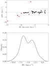 |
Fig. 1. Top: radial velocity residuals between this work and APOGEE (ΔRV = RV this work – RV APOGEE). The radial velocity measurements that are not compatible within 5σ uncertainties are indicated in red. Bottom: radial velocity distribution of the bona fide sample. We used a Gaussian kernel density with a bandwidth of 0.25 km s−1, similar to the radial velocity precision of the sample. |
The final distribution of radial velocities is multivariate because it includes several kinematic populations (see Fig. 1, bottom). Despite the relatively wide spread of the population, several sources have a radial velocity measurement that is clearly not consistent with this region. As our sample has been selected with extremely precise Gaia astrometry and photometry, we expect a very low contamination rate (≲1%, Miret-Roig et al. 2022). Therefore, we defined a radial velocity filtering criterion to exclude outliers in the radial velocity distribution. We kept only the radial velocity measures in the 90% central distribution, and discarded the radial velocities that fall outside the percentiles p5, p95. These 108 sources are candidates to be spectroscopic binaries (with insufficient observations to be detected) or for which the measurements are problematic.
2.3. Bona fide sample
To identify the substructure of this region and obtain precise dynamical traceback ages, we defined a subsample of stars with the most precise data. We only considered sources classified as members by Miret-Roig et al. (2022) using Gaia astrometry. We applied the filtering criteria described in Fabricius et al. (2021) to identify potential non-single objects and 5σ outliers in parallax or proper motion. These criteria are based on the renormalised unit weight error (RUWE) parameter (ruwe < 1.4) and two image-level indicators (ipd_gof_harmonic_amplitude < 0.1 and ipd_frac_multi_peak ≤ 2). After this filtering, the sample contains 2190 sources (78% of the initial sample) with 5D Gaia astrometry and 670 sources with 6D phase space data.
3. Groups in the 6D phase space
Gaia has demonstrated that the spatial and kinematic structure of associations and star-forming regions is highly complex. In particular, several studies have recently analysed the region of Upper Scorpius finding different groups in this region (e.g., Damiani et al. 2019; Kerr et al. 2021; Squicciarini et al. 2021; Ratzenböck 2022; Briceño-Morales & Chanamé 2022). The phase space (XYZUVW) is the best space to unravel the spatial and kinematic complexity because it avoids problems such as projection effects. The main drawback of this space is that it requires accurate radial velocities, which are not available in the same quantity and quality as the 5D astrometry. Working in the phase space with limited radial velocities can then introduce some biases due to the incompleteness of the sample. For instance, the Gaia radial velocities are magnitude limited and the APOGEE radial velocities are spatially limited with the footprint of the survey. The novelty of our study with respect to previous ones is that it searches for substructures in a 6D space in which we can include the sources with missing radial velocity by marginalising over the missing information. This is possible in a representation space that includes the radial velocity and not a transformation of it. This allows us to work in a complete 6D space and include a large fraction of the members in the region at the same time. Our methodology also accounts for the observational uncertainties.
We used a Gaussian mixture model (GMM) in the 3D Galactic Cartesian positions, 2D Galactic tangential velocities, and radial velocity space to classify all the members of Upper Scorpius and Ophiuchus into different substructures. We infer the parameters of this GMM using the algorithm developed by Olivares et al. (2018, see their Sect. 2.1.1). There is an advantage to using this algorithm in that it also takes into account the sources with missing radial velocity to find the best model of the observations, minimising any possible observational bias. First, we fitted the GMM to the 2 190 sources in the 5D bona fide sample (30% of which have a radial velocity measurement in our final catalogue, excluding sources with large uncertainties and binaries; see Table 1 and Sect. 2). Having established the best final model, we classified the complete sample of sources.
We explored all models with a number of components between 1 and 17. We decided to work with the seven-component solution, which is the one with the lowest Bayesian information criteria (BIC). We also analysed the remaining models and found that, in more complex models, the new components are wider and tend to catch sources in the outskirts of the distribution of parameters in the representation space. These models represent less reliable populations because they are likely overfitting the data. We fitted the GMM with five different seeds and in all cases we find groups with similar weights, means, and covariance matrix. We repeated the same procedure in a different representation space, XYZUVW, obtaining similar results. The disadvantage of this space is that we cannot include the sources with missing information in the radial velocity, and therefore we prefer the former analysis. In Fig. 2, we show the distribution of the groups projected on the plane of the sky, where we also indicate the position of the giant star that gives the group its name. Several of these B-type stars were initially classified in the group of σ Sco, which is very extended in the position space. However, the astrometry of these very bright stars is less precise and we reclassified them into their closest group in the plane of the sky. In Fig. A.1, we show the distribution of groups in the representation space and in Table 3, we summarise the mean properties of the groups we found.
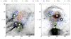 |
Fig. 2. Distribution of the groups in the plane of the sky in Galactic coordinates. The positions of the B-type stars that give their names to the groups are indicated by the white circles. We show the location of the τ Sco star discussed in the main text. The background image shows the emission in radio, at 857 GHz (left, Planck Collaboration I 2020), and in Hα (right, Finkbeiner 2003). |
Groups identified in the region of Upper Scorpius and Ophiuchus.
The dispersion in the positions in the radial direction (σX) is slightly larger than in the other two directions. This is not surprising because the radial direction is the closest to the line of sight. The median uncertainty in the radial (X) positions is 1 pc, which is more than twice the median uncertainty in both the azimuthal (Y) and vertical (Z) positions. The three components of the Cartesian velocities have similar precisions of a few hundred meters per second due to the filtering in radial velocities that we applied (see Sect. 2). The dispersion in the positions of the groups α Sco, σ Sco, and π Sco is larger than the rest, indicating that these groups might be older populations that started to disperse into the Galactic field or that they were born further apart (Ward et al. 2020; Wright et al. 2022). The groups σ Sco and π Sco occupy the entire area analysed in this work, suggesting that we might be seeing only part of them. This could have implications for the determination of the dynamical traceback ages as we discuss in the following sections. The group of σ Sco has the largest dispersion in velocities, which could indicate that this group is slightly more contaminated.
3.1. Comparison with previous studies
We cross-matched our list of members with the three recent studies that also identified several spatial and kinematic groups in this region, namely Kerr et al. (2021), Squicciarini et al. (2021), and Ratzenböck (2022). In Table A.1 we relate the names of the groups in our study to the names given in previous works. We identified the groups in previous studies that share the majority of members with our groups, but there are always small differences in the list of members of each group. The groups of ρ Oph, ν Sco, β Sco, and δ Sco generally agree well in all studies. This strongly validates these groups, because each study used a different methodology and representation space. On the contrary, the more dispersed groups of α Sco, σ Sco, and π Sco seem more mixed and different authors have separated them differently. Therefore, the results of these three groups should be considered with slightly more caution.
4. Dynamical traceback ages
We used the methodology described in Miret-Roig et al. (2018, 2020) to compute the dynamical traceback age for each of the groups identified in this study. In short, this methodology uses the present 3D positions and 3D velocities of individual stars and computes the stellar orbits back in time with a Galactic potential. We used two different 3D Milky Way potentials, namely MWPotential14 (Bovy 2015) and McMillan17 (McMillan 2017), and obtained the same results. We performed the orbital integration with the galpy software3 (Bovy 2015). We refer to Miret-Roig et al. (2020) for more details on the impact of Galactic potentials on the dynamical traceback age of young stellar associations.
We define the dynamical traceback age as the time when a group of stars was most concentrated in the past, that is, when the size of the group was at its minimum. We measured the size of a group of stars with a robust estimate of the covariance matrix (Σ, the ‘minimum covariance determinant’ from Sklearn Pedregosa et al. 2011), which reduces the impact of outliers in the sample, and the three functions defined in Miret-Roig et al. (2020).
-
The sizes in the radial, azimuthal, and vertical directions (Sx, Sy, Sz) are the square root of the diagonal terms of the covariance matrix in each direction.
-
The trace covariance matrix size (STCM) is defined as:
![Mathematical equation: $$ \begin{aligned} S_{\rm TCM} = \left[ \frac{ {{\,\mathrm{Tr}\,}}(\mathbf {\Sigma} )}{3} \right]^{1/2}, \end{aligned} $$](/articles/aa/full_html/2022/11/aa44709-22/aa44709-22-eq1.gif) (1)
(1)where Tr(Σ) is the sum of elements on the main diagonal (from the upper left to the lower right) of Σ.
-
The determinant covariance matrix size (SDCM) is defined as:
![Mathematical equation: $$ \begin{aligned} S_{\rm DCM} = \left[ \det (\mathbf {\Sigma} ) \right]^{1/6}\!. \end{aligned} $$](/articles/aa/full_html/2022/11/aa44709-22/aa44709-22-eq2.gif) (2)
(2)
We show the size of each group as a function of time using these three functions in Fig. A.2 (left panels). We computed the dynamical traceback age with a 1000 bootstrap repetition with replacement, each time taking the same number of sources as the number of members in the group. This strategy accounts for the uncertainty in the dynamical traceback age from contamination in group members, which dominates the observational uncertainties and the uncertainties on different modern models of the Galactic potential (Miret-Roig et al. 2020). For each bootstrap repetition, we measured a dynamical traceback age which is shown in the age distributions in Fig. A.2 (right panels). In some cases, the age distributions are wide or bimodal, indicating that there might be a degree of contamination in the sample.
We measured a dynamical traceback age for each group using the five size estimators (Sx, Sy, Sz, STCM, SDCM). In each case, we report the median and standard deviation of the dynamical traceback age distribution in Table 4. The ages obtained with the determinant and the trace contain the full 3D information and are compatible within the uncertainties. Therefore, we use the dynamical traceback age obtained from the trace for the rest of the discussion, which is similar to the approach described in Miret-Roig et al. (2020). In Fig. 3, we show the dynamical traceback age distribution for each of the groups. We observe an age gradient among different groups that is statistically significant, suggesting that star formation has been a sequential process – with several star formation bursts – over the past 5 Myr. Similar age gradients have been observed in other nearby star forming regions, as in Orion (Mathieu 2008; Großschedl et al. 2021), Vela (Cantat-Gaudin et al. 2019; Armstrong et al. 2022), Perseus (Pavlidou et al. 2021), and Cygnus (Quintana & Wright 2022).
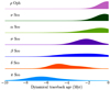 |
Fig. 3. Dynamical traceback age distribution obtained for each of the groups using the trace as the size estimator. |
Dynamical traceback age summary.
Recently, Squicciarini et al. (2021) also measured kinematic traceback ages4 of different groups in Upper Scorpius. The main differences between our method and theirs are that: (i) they report the ages obtained with a 4D analysis (RA, Dec, tangential velocity in RA, Dec; see their Table 4, although they did some tests in 6D); (ii) they used a different strategy to measure the size of a group; and (iii) they did not use a Galactic potential to compute the orbits of stars back in time. For the groups where we have similar membership lists (ρ Oph, ν Sco, β Sco, and δ Sco) we find results that are compatible within the uncertainties. The main difference is that in our study, the δ Sco group is 2 Myr older than the β Sco group.
4.1. Validation of the age gradient with isochrones and possible origin of a zero-point shift
A common technique to determine stellar ages is the use of evolutionary models, which has proven to be very successful for intermediate and old clusters (see e.g., Bossini et al. 2019; Cantat-Gaudin et al. 2020). However, very young stars (< 20 Myr) are often variable (due to activity) and affected by interstellar extinction (which changes spatially in this region; see Fig. 2). These and other effects make photometric ages for such young objects notoriously difficult to estimate (e.g., Jeffries et al. 2014, 2021; Binks et al. 2022). Additionally, stellar evolution models are especially uncertain at very young ages, making isochrone fitting less ideal for those cases (Barrado 2016). Determining isochronal ages from evolutionary models is beyond the scope of this work, but we still use colour–magnitude diagrams (CMDs) to validate the relative age scale determined in this section (Fig. 3).
In Fig. 4, we show the CMD of the seven groups identified in this work on top of the PARSEC isochrone (Marigo et al. 2017), corresponding to the dynamical traceback ages determined in this study. Visual inspection reveals that ρ Oph and ν Sco are the youngest groups. The groups of α Sco, σ Sco, β Sco, and δ Sco have intermediate ages and the scatter in the CMDs makes it difficult to determine relative differences between these four groups. The most likely reasons for this scatter are extinction, which is spatially variable (see Fig. 2, left panel), and stellar variability. However, a slight contamination of the membership could also be responsible for part of the scatter. Finally, the group of π Sco is the oldest in this region according to the CMD. The relative age scale obtained in this study from dynamical traceback ages generally agrees with the one observed in the CMD within the uncertainties.
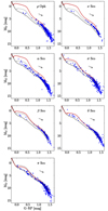 |
Fig. 4. Colour magnitude diagram of the members of the groups identified in this study. The PARSEC isochrones corresponding to the dynamical traceback ages determined in this study are indicated in red. The PARSEC isochrones at 5 and 20 Myr and the 1 mag extinction vector are also indicated. |
Looking at Fig. 4, we see that the isochronal ages of these groups might be a few million years older than the dynamical traceback ages determined in this study. This is especially true for π Sco, which could have an age of around 20 Myr according to evolutionary models. However, this association likely extends beyond the area covered by our study, and our spatial selection could bias the dynamical traceback age. We believe that gravitational interactions between different groups, stellar feedback, and the dissipation of the parent gas must play an important role in explaining the smaller age differences in the rest of the groups. These effects are not accounted for in our study and can produce perturbations in the orbits of individual stars, which would affect the estimated dynamical traceback ages. We estimate that these perturbations should be of the order of the age of the ρ Oph group (1–3 Myr, Greene & Meyer 1995) for which we could not determine a dynamical traceback age. Adding this 1–3 Myr offset to the dynamical traceback ages obtained for the rest of the groups reconciles the ages measured in this study with isochronal age measurements in this region. However, we add a last word of caution because isochronal ages for young stellar associations are also affected by other limitations, as we discuss at the beginning of this section.
Another technique used to measure kinematic ages consists of measuring the correlation between the velocity and position of all members in a group (Torres et al. 2006; Mamajek & Bell 2014; Miret-Roig et al. 2020). We fitted a linear relation between the Cartesian heliocentric positions (XYZ) and velocities (UVW) independently to each of the three directions (Galactic centre, Galactic rotation, and Galactic north pole). Although we find signs of expansion in all groups, we are unable to determine precise expansion ages for any group. We interpret this as most groups being too young to have undergone a significant expansion that can be measured at present with this simple method.
5. Star formation history
In this section, we investigate the star formation history of the different groups identified in this study. First, we compute the orbit of the centre of each group using a 3D Galactic potential. Then, we discuss possible sources of feedback that could have triggered star formation in this region and perturbed the trajectories of stars.
5.1. Orbital traceback analysis
We computed the orbit of the centre of each group 20 Myr back in time using the same strategy as that described in Sect. 4 for individual stars. In Fig. 5 (interactive)5, we show the 3D orbits of the centre of each group where the coloured part of the orbit corresponds to the trajectory of the association from the present back to the birth place as determined in this study.
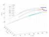 |
Fig. 5. Orbits back in time of the centre of each of the groups identified in this study. The coloured trajectories indicate the orbit of the groups from the present back to the birth time determined in this study within the reported uncertainties in the dynamical ages. The grey trajectories indicate the orbit of the groups from the birth time determined in this study to 20 Myr ago. |
Upper Scorpius is divided into four different groups according to our analysis, namely ν Sco, σ Sco, β Sco, and δ Sco. The groups of β Sco and δ Sco were closest 4 Myr ago, which is compatible with the dynamical traceback ages of these two groups (2.5 ± 1.6 Myr and 4.6 ± 1.1 Myr, respectively), when their centres were at 7 pc. The group of ν Sco (0.3 ± 0.5 Myr) was closest to the group of β Sco (2.5 ± 1.6 Myr) 4.5 Myr ago at only 1 pc distance. The orbit of the centre of σ Sco (2.1 ± 0.7 Myr) intersects with δ Sco (4.6 ± 1.1 Myr) around 20 Myr ago but these two groups were closer than 10 pc 3 Myr ago. This clearly suggests that these four groups likely have a common origin.
ρ Oph is the youngest group in our study. We were not able to estimate a dynamical traceback age because this method requires that the association has undergone a significant expansion and this is not the case for this group, which is likely still gravitationally bound (Rigliaco et al. 2016). The orbit of the centre of ρ Oph shows that it has a common origin with Upper Scorpius, because it was at only 1 pc from δ Sco 5 Myr ago, similar to the age of this second group. Both the ages obtained in this study and the fact that ρ Oph is the youngest group in Upper Scorpius support the formation scenario proposed by Preibisch & Zinnecker (1999).
The group π Sco is a population located at a distance of 120 pc, in front of Upper Scorpius and Ophiuchus. Our dynamical traceback age (6.3 ± 1.4 Myr) suggests that it is the oldest group in this study, which is confirmed by the location of the members in this group in a CMD. The group of α Sco has a dynamical traceback age (1.0 ± 1.2 Myr) similar to the young groups in Upper Scorpius but the CMD indicates that it could be slightly older. These two groups were closest 5 Myr ago when their centres were at 20 pc. Although their orbits seem to cross in the static version of Fig. 5, they are never at the same place at the same time (see the interactive version). The groups of π Sco and α Sco have different orbits from the other groups in this study, suggesting that they have a different origin. We propose that they could have an origin related to other associations in the Sco-Cen complex. We traced the 3D positions and velocities of Upper Centaurus Lupus and Lower Centaurus Crux from Gagné et al. (2018) back in time and found that the groups of π Sco and α Sco were closer to Upper Centaurus Lupus 15–20 Myr ago.
5.2. Stellar feedback
The orbits discussed in this study are based on the current positions and velocities of stars and a 3D Galactic potential; they do not take into account gravitational interactions between different groups and stellar feedback, which might be important in some cases. In Fig. 2 (right panel), we see the groups identified in this study coinciding with Hα emission, tracing the HII regions in this area very likely powered by the four early B-type stars (δ Sco, π Sco, σ Sco and τ Sco). To test whether these HII regions are generated from the photoionisation of these massive stars, we compared their sizes with the radius of Strömgren spheres (Strömgren 1939), which are defined by the equation:
 (3)
(3)
where QH is the hydrogen-ionising photon luminosities computed by adopting the calibration in Smith (2006), α = 3.09 × 10⁻¹³ cm3 s−1 is the recombination coefficient (for a kinetic temperature of 8000 K, Spitzer 1978), and np = 10 protons cm−3 is the proton density (Alves, in prep.). The Strömgren radii calculated are listed in Table 5.
Strömgren radius.
The sizes of the HII regions measured with Eq. (3) are similar to the measured physical sizes on the Hα map, confirming the assumption that photoionisation by the current massive stars in the region is responsible for the observed Hα emission. Intriguingly, there is no Hα emission around the B1V+B2V β Sco system. This could indicate that the local density is very low, although more work is needed to solve this mystery. Currently, the groups of β Sco and ν Sco are close but outside the HII region of δ Sco, suggesting that the present ionisation alone is unlikely to be triggering star formation in these two groups. However, around 4 Myr ago, the centres of the groups β Sco and ν Sco were at the boundaries of the HII region of δ Sco, suggesting that the photoionisation and stellar winds of δ Sco could have compressed the molecular gas available after the formation of the δ Sco group, possibly triggering the formation of the groups β Sco and ν Sco.
In addition to the HII regions surrounding the early B-type stars, we also see other structures in the Hα map, such as the large shell at the top of the image in Fig. 2 (right panel). This shell could be the remnant of other sources of feedback in the region, although a dedicated analysis goes beyond the goal of this paper. The event that created this shell, and not necessarily the phenomenon that currently makes it shine in Hα, probably had an important impact on the SFH of the region. About 15 supernovae are known to have exploded in this region (Breitschwerdt et al. 2016; Zucker et al. 2022), and these probably had an important impact on its SFH. The well-known runaway star ζ Oph is the smoking gun of a supernova that exploded about 1–2 Myr ago (Neuhäuser et al. 2020), probably the last supernova explosion in the region.
In this paper, we analyse the youngest region of Sco-Cen, Upper-Scorpius, which contains about one-third of the sources in the entire Sco-Cen OB association. A detailed study of the other neighbouring groups in Sco-Cen will help to shed light on the complete picture; as we have discussed, some groups identified in this study could be older and related to the rest of Sco-Cen. Also other young local associations such as β Pictoris have been suggested to have a common origin with Sco-Cen (Fernández et al. 2008; Miret-Roig et al. 2018). Finally, the large context in which the Sco-Cen association is embedded is relevant to our understanding of the origins of this benchmark association. The Sco-Cen complex is found at the end of the ‘Split’, a large-scale gas structure (Lallement et al. 2019), and next to an even larger gas structure called the ‘Radcliffe Wave’ (Alves et al. 2020), which is likely the gas reservoir of the Orion Arm of the Milky Way (Swiggum et al. 2022). A full analysis of Sco-Cen using the approach followed in this paper is warranted and is likely to reveal important pieces of the SFH of the closest OB association, and the star formation in the Sun’s neighbourhood.
5.3. Proposed star-formation scenario
Taking the orbital traceback analysis as a first-order approximation of the paths of the groups back in time, and complementing this information with the insights into stellar feedback, we propose the following star-formation scenario, which is also illustrated in Fig. 6.
-
Around 5–6 Myr ago, the early B-type star δ Sco ionised the medium around it, creating an HII region.
-
We propose that in the past, the star-forming cloud extended towards the area currently occupied by the groups ν Sco and β Sco, and that the combined effect of (possible) supernovae from the δ Sco group, stellar winds, and the bubble of ionised material around δ Sco then compressed the cloud, triggering star formation mostly towards the area of β Sco.
-
Around 4 Myr ago, the group of β Sco was born. This is the time when it was closest to δ Sco, which is consistent with the dynamical traceback age determined in this study.
-
Over the last 2 Myr, star formation has progressed towards the area of ν Sco, probably triggered by the feedback of both the δ Sco and β Sco events. Given that there is little dense gas to the west of ν Sco, this is perhaps the last significant star-formation event in the region.
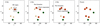 |
Fig. 6. Schema representing the proposed star-formation scenario in Upper Scorpius. |
This star-formation scenario is compatible with a triggered star-formation process similar to the one presented by Preibisch et al. (2008) and with the predictions of the ‘surround and squash’ mechanism proposed by Krause et al. (2018). The latter predicts gravitationally unbound groups with substructures that have coherent kinematics, as we observed in our sample.
6. Conclusions
We present the first detailed study of the SFH of Upper Scorpius and Ophiuchus in 7D (3D positions, 3D velocities and age). Combining Gaia DR3 astrometry and radial velocities with precise ground-based radial velocities from APOGEE DR17 and our own observations, we identified seven groups using 3D kinematics and 3D spatial information. We integrated the orbits of individual stars back in time with a 3D Galactic potential and measured dynamical traceback ages (i.e. the time when the stars in a group were most concentrated in the past; Miret-Roig et al. 2018, 2020). We find an age gradient between different groups that is statistically significant and that also correlates with an age gradient in colour–magnitude diagrams. We find a dynamical traceback age of Upper Scorpius of younger than 5 Myr.
We studied the SFH of this complex by computing the orbit of the centre of each group back in time. We find that the Upper Scorpius association splits into four groups, namely ν Sco, β Sco, σ Sco, and δ Sco, which share a common origin. We speculate that feedback from massive stars in the δ Sco group could have triggered star formation first in β Sco and then in ν Sco. The origin of ρ Oph can also be related to Upper Scorpius according to its orbit back in time, in agreement with propositions put forward in previous studies (Preibisch & Zinnecker 1999; Preibisch et al. 2002). The two groups of α Sco and π Sco seem to have a different origin, which we relate to other regions of the Sco-Cen complex (Upper Centaurus-Lupus).
The SFH presented in this study constitutes a development of the early work of Preibisch & Zinnecker (1999). We confirm their global picture but we show that the history of the region is much more complex than in their scenario. Still, the final picture is far from complete because a detailed analysis of stellar feedback and gas dynamics is missing, which will have an important impact on the large-scale gas motion of the region.
Interactive Figure
Interactive image associated with Fig. 5 Access Supplementary Material
We included the ρ Oph and χ Oph B-type stars, which are well-known members of the young association but are not identified as members by the study because of their binary nature and extinction. They both have membership probabilities of greater than 0.5 but below the threshold established in that study to avoid a large fraction of contaminants.
We used the inverse of the squared uncertainty as weights (wi = (σRV, i)−2) and the uncertainty in the weighted average as σRV, WA = [Σiwi]−1.
We refer to their ages as kinematic traceback ages because they did not use a Galactic potential to trace back the orbits of stars. We note that they use the term ‘kinematic ages’ to refer to their results.
An interactive version of this figure is available online.
Acknowledgments
The authors thank the anonymous referee for very useful comments that helped to improve the presentation of these results. The authors thank Cameren Swiggum for producing the interactive version of Fig. 5. This research has received funding from the European Research Council (ERC) under the European Union’s Horizon 2020 research and innovation programme (grant agreement No 682903, P.I. H. Bouy), and from the French State in the framework of the ‘Investments for the future’ Program, IdEx Bordeaux, reference ANR-10-IDEX-03-02. We thank NVIDIA Corporation for their support, in particular, the donation of one of the Titan Xp GPUs used for this research. P.A.B. Galli acknowledges financial support from São Paulo Research Foundation (FAPESP) under grants 2020/12518-8 and 2021/11778-9. J.O. acknowledges financial support from ‘Ayudas para contratos postdoctorales de investigación UNED 2021’. DB has been partially funded by MCIN/AEI/10.13039/501100011033 grants PID2019-107061GB-C61 and MDM-2017-0737. This work has made use of data from the European Space Agency (ESA) mission Gaia (https://www.cosmos.esa.int/gaia), processed by the Gaia Data Processing and Analysis Consortium (DPAC, https://www.cosmos.esa.int/web/gaia/dpac/consortium). Funding for the DPAC has been provided by national institutions, in particular the institutions participating in the Gaia Multilateral Agreement. Based on observations collected at the European Organisation for Astronomical Research in the Southern Hemisphere under ESO programmes 099.A-9029, 083.D-0034, 083.A-9013, 083.A-9017, 093.A-9029, 077.C-0258, 076.A-9018, 079.A-9002, 072.A-9012, 087.C-0315, 084.A-9016, 081.C-2003, 073.C-0355, 094.A-9012, 093.A-9008, 073.C-0337, 086.D-0449, 082.D-0061, 087.D-0099, 089.D-0153, 093.A-9006, 083.A-9003, 084.D-0067, 179.C-0197, 077.D-0477, 091.C-0713, 076.D-0172, 075.C-0399, 072.A-9006, 078.C-0011, 077.C-0138, 092.A-9029, 091.C-0216, 178.D-0361, 0101.A-9003, 098.C-0739, 082.C-0390, 081.C-0779, 077.D-0085, 099.D-0380, 0104.C-0418,0100.D-0273,1101.C-0557, 099.D-0628, 188.B-3002, 081.C-0708, 075.C-0256, 073.C-0179, 075.B-0863, 075.C-0551, 65.I-0404, 69.C-0481, 65.L-0199, 67.C-0160, 69.B-0108, 71.C-0068, 097.C-0409, 084.C-1002, 079.C-0556, 083.D-0689, 266.D-5655, 073.C-0138, 081.C-0475, 077.C-0323, 093.C-0476, 085.C-0524, 093.C-0658, 075.C-0272, 097.C-0979, 082.C-0005, 081.D-0904, 079.C-0375, 093.D-0279, 081.C-0222, 075.C-0292, 089.C-0299, 0102.C-0040. Based on spectral data retrieved from the ELODIE archive at Observatoire de Haute-Provence (OHP, http://atlas.obs-hp.fr/elodie/). Based on observations obtained withCHIRON at the 1.5 m Telescope in Cerro Tololo operated by the SMARTS Consortium (P.I. Bouy, NOIRLab Programs 2020A-0094 and 2021A-0011) with Hermes at the Mercatortelescope (P.I. Barrado, Program 5-Mercator1/21A).
References
- Abdurro’uf, A., Accetta, K., Aerts, C., et al. 2022, ApJS, 259, 35 [NASA ADS] [CrossRef] [Google Scholar]
- Alves, J., Zucker, C., Goodman, A. A., et al. 2020, Nature, 578, 237 [NASA ADS] [CrossRef] [Google Scholar]
- Armstrong, J. J., Wright, N. J., Jeffries, R. D., Jackson, R. J., & Cantat-Gaudin, T. 2022, MNRAS, 517, 5704 [NASA ADS] [CrossRef] [Google Scholar]
- Asensio-Torres, R., Currie, T., Janson, M., et al. 2019, A&A, 622, A42 [NASA ADS] [CrossRef] [EDP Sciences] [Google Scholar]
- Barenfeld, S. A., Carpenter, J. M., Ricci, L., & Isella, A. 2016, ApJ, 827, 142 [Google Scholar]
- Barrado, D. 2016, EAS Pub. Ser., 80–81, 115 [CrossRef] [EDP Sciences] [Google Scholar]
- Binks, A. S., Jeffries, R. D., Sacco, G. G., et al. 2022, MNRAS, 513, 5727 [NASA ADS] [Google Scholar]
- Bossini, D., Vallenari, A., Bragaglia, A., et al. 2019, A&A, 623, A108 [NASA ADS] [CrossRef] [EDP Sciences] [Google Scholar]
- Bovy, J. 2015, ApJS, 216, 29 [NASA ADS] [CrossRef] [Google Scholar]
- Breitschwerdt, D., Feige, J., Schulreich, M. M., et al. 2016, Nature, 532, 73 [NASA ADS] [CrossRef] [Google Scholar]
- Briceño-Morales, G., & Chanamé, J. 2022, arXiv e-prints [arXiv:2205.01735] [Google Scholar]
- Cantat-Gaudin, T., Mapelli, M., Balaguer-Núñez, L., et al. 2019, A&A, 621, A115 [NASA ADS] [CrossRef] [EDP Sciences] [Google Scholar]
- Cantat-Gaudin, T., Anders, F., Castro-Ginard, A., et al. 2020, A&A, 640, A1 [NASA ADS] [CrossRef] [EDP Sciences] [Google Scholar]
- Damiani, F., Prisinzano, L., Pillitteri, I., Micela, G., & Sciortino, S. 2019, A&A, 623, A112 [NASA ADS] [CrossRef] [EDP Sciences] [Google Scholar]
- David, T. J., Hillenbrand, L. A., Gillen, E., et al. 2019, ApJ, 872, 161 [Google Scholar]
- de Geus, E. J., de Zeeuw, P. T., & Lub, J. 1989, A&A, 216, 44 [NASA ADS] [Google Scholar]
- de Zeeuw, P. T., Hoogerwerf, R., de Bruijne, J. H. J., Brown, A. G. A., & Blaauw, A. 1999, AJ, 117, 354 [Google Scholar]
- Donati, J. F., Howarth, I. D., Jardine, M. M., et al. 2006, MNRAS, 370, 629 [NASA ADS] [CrossRef] [Google Scholar]
- Elmegreen, B. G., & Lada, C. J. 1977, ApJ, 214, 725 [Google Scholar]
- Esplin, T. L., Luhman, K. L., Miller, E. B., & Mamajek, E. E. 2018, AJ, 156, 75 [NASA ADS] [CrossRef] [Google Scholar]
- Fabricius, C., Luri, X., Arenou, F., et al. 2021, A&A, 649, A5 [NASA ADS] [CrossRef] [EDP Sciences] [Google Scholar]
- Fang, Q., Herczeg, G. J., & Rizzuto, A. 2017, ApJ, 842, 123 [Google Scholar]
- Feiden, G. A. 2016, A&A, 593, A99 [NASA ADS] [CrossRef] [EDP Sciences] [Google Scholar]
- Fernández, D., Figueras, F., & Torra, J. 2008, A&A, 480, 735 [NASA ADS] [CrossRef] [EDP Sciences] [Google Scholar]
- Finkbeiner, D. P. 2003, ApJS, 146, 407 [Google Scholar]
- Gagné, J., Mamajek, E. E., Malo, L., et al. 2018, ApJ, 856, 23 [Google Scholar]
- Gaia Collaboration (Prusti, T., et al.) 2016, A&A, 595, A1 [NASA ADS] [CrossRef] [EDP Sciences] [Google Scholar]
- Gaia Collaboration (Vallenari, A., et al.) 2022, A&A, accepted, https://doi.org/10.1051/0004-6361/202243940 [Google Scholar]
- Garrison, R. F. 1967, ApJ, 147, 1003 [NASA ADS] [CrossRef] [Google Scholar]
- Grasser, N., Ratzenböck, S., Alves, J., et al. 2021, A&A, 652, A2 [NASA ADS] [CrossRef] [EDP Sciences] [Google Scholar]
- Greene, T. P., & Meyer, M. R. 1995, ApJ, 450, 233 [NASA ADS] [CrossRef] [Google Scholar]
- Großschedl, J. E., Alves, J., Meingast, S., & Herbst-Kiss, G. 2021, A&A, 647, A91 [NASA ADS] [CrossRef] [EDP Sciences] [Google Scholar]
- Herczeg, G. J., & Hillenbrand, L. A. 2015, ApJ, 808, 23 [Google Scholar]
- Jeffries, R. D., Jackson, R. J., Cottaar, M., et al. 2014, A&A, 563, A94 [NASA ADS] [CrossRef] [EDP Sciences] [Google Scholar]
- Jeffries, R. D., Jackson, R. J., Sun, Q., & Deliyannis, C. P. 2021, MNRAS, 500, 1158 [Google Scholar]
- Katz, D., Sartoretti, P., Guerrier, A., et al. 2022, A&A, submitted [arXiv:2206.05902] [Google Scholar]
- Kerr, R. M. P., Rizzuto, A. C., Kraus, A. L., & Offner, S. S. R. 2021, ApJ, 917, 23 [NASA ADS] [CrossRef] [Google Scholar]
- Krause, M. G. H., Burkert, A., Diehl, R., et al. 2018, A&A, 619, A120 [NASA ADS] [CrossRef] [EDP Sciences] [Google Scholar]
- Lallement, R., Babusiaux, C., Vergely, J. L., et al. 2019, A&A, 625, A135 [NASA ADS] [CrossRef] [EDP Sciences] [Google Scholar]
- Loren, R. B. 1989, ApJ, 338, 902 [CrossRef] [Google Scholar]
- Luhman, K. L. 2022, AJ, 163, 24 [NASA ADS] [CrossRef] [Google Scholar]
- Maíz Apellániz, J., Barbá, R. H., Fariña, C., et al. 2021, A&A, 646, A11 [NASA ADS] [CrossRef] [EDP Sciences] [Google Scholar]
- Majewski, S. R., Schiavon, R. P., Frinchaboy, P. M., et al. 2017, AJ, 154, 94 [NASA ADS] [CrossRef] [Google Scholar]
- Mamajek, E. E., & Bell, C. P. M. 2014, MNRAS, 445, 2169 [Google Scholar]
- Marigo, P., Girardi, L., Bressan, A., et al. 2017, ApJ, 835, 77 [Google Scholar]
- Mathieu, R. D. 2008, in Handbook of Star Forming Regions, Volume I, ed. B. Reipurth, 4, 757 [NASA ADS] [Google Scholar]
- McMillan, P. J. 2017, MNRAS, 465, 76 [NASA ADS] [CrossRef] [Google Scholar]
- Miret-Roig, N., Antoja, T., Romero-Gómez, M., & Figueras, F. 2018, A&A, 615, A51 [NASA ADS] [CrossRef] [EDP Sciences] [Google Scholar]
- Miret-Roig, N., Galli, P. A. B., Brandner, W., et al. 2020, A&A, 642, A179 [NASA ADS] [CrossRef] [EDP Sciences] [Google Scholar]
- Miret-Roig, N., Bouy, H., Raymond, S. N., et al. 2022, Nat. Astron., 6, 89 [NASA ADS] [CrossRef] [Google Scholar]
- Morgan, W. W., & Keenan, P. C. 1973, ARA&A, 11, 29 [NASA ADS] [CrossRef] [Google Scholar]
- Neuhäuser, R., Gießler, F., & Hambaryan, V. V. 2020, MNRAS, 498, 899 [CrossRef] [Google Scholar]
- Olivares, J., Sarro, L. M., Moraux, E., et al. 2018, A&A, 617, A15 [NASA ADS] [CrossRef] [EDP Sciences] [Google Scholar]
- Pavlidou, T., Scholz, A., & Teixeira, P. S. 2021, MNRAS, 503, 3232 [NASA ADS] [CrossRef] [Google Scholar]
- Pecaut, M. J., Mamajek, E. E., & Bubar, E. J. 2012, ApJ, 746, 154 [Google Scholar]
- Pedregosa, F., Varoquaux, G., Gramfort, A., et al. 2011, J. Mach. Learn. Res., 12, 2825 [Google Scholar]
- Pérez, M. R., van den Ancker, M. E., de Winter, D., & Bopp, B. W. 2004, A&A, 416, 647 [NASA ADS] [CrossRef] [EDP Sciences] [Google Scholar]
- Planck Collaboration I. 2020, A&A, 641, A1 [NASA ADS] [CrossRef] [EDP Sciences] [Google Scholar]
- Preibisch, T., & Mamajek, E. 2008, in Handbook of Star Forming Regions, Volume II, ed. B. Reipurth, 5, 235 [NASA ADS] [Google Scholar]
- Preibisch, T., & Zinnecker, H. 1999, AJ, 117, 2381 [NASA ADS] [CrossRef] [Google Scholar]
- Preibisch, T., Brown, A. G. A., Bridges, T., Guenther, E., & Zinnecker, H. 2002, AJ, 124, 404 [NASA ADS] [CrossRef] [Google Scholar]
- Quintana, A. L., & Wright, N. J. 2022, MNRAS, 515, 687 [NASA ADS] [CrossRef] [Google Scholar]
- Ratzenböck, S., Möller, T., Großschedl, J. E., et al. 2022, A&A, submitted [Google Scholar]
- Ratzka, T., Köhler, R., & Leinert, C. 2005, A&A, 437, 611 [NASA ADS] [CrossRef] [EDP Sciences] [Google Scholar]
- Richert, A. J. W., Getman, K. V., Feigelson, E. D., et al. 2018, MNRAS, 477, 5191 [NASA ADS] [CrossRef] [Google Scholar]
- Rigliaco, E., Wilking, B., Meyer, M. R., et al. 2016, A&A, 588, A123 [NASA ADS] [CrossRef] [EDP Sciences] [Google Scholar]
- Rizzuto, A. C., Ireland, M. J., Dupuy, T. J., & Kraus, A. L. 2016, ApJ, 817, 164 [NASA ADS] [CrossRef] [Google Scholar]
- Rosero, V., Prato, L., Wasserman, L. H., & Rodgers, B. 2011, AJ, 141, 13 [NASA ADS] [CrossRef] [Google Scholar]
- Slesnick, C. L., Hillenbrand, L. A., & Carpenter, J. M. 2008, ApJ, 688, 377 [NASA ADS] [CrossRef] [Google Scholar]
- Smith, N. 2006, MNRAS, 367, 763 [Google Scholar]
- Spitzer, L. 1978, Physical Processes in the Interstellar Medium (New York: Wiley) [Google Scholar]
- Squicciarini, V., Gratton, R., Bonavita, M., & Mesa, D. 2021, MNRAS, 507, 1381 [NASA ADS] [CrossRef] [Google Scholar]
- Stauffer, J., Rebull, L. M., Cody, A. M., et al. 2018, AJ, 156, 275 [NASA ADS] [CrossRef] [Google Scholar]
- Strömgren, B. 1939, ApJ, 89, 526 [CrossRef] [Google Scholar]
- Sullivan, K., & Kraus, A. L. 2021, ApJ, 912, 137 [NASA ADS] [CrossRef] [Google Scholar]
- Swiggum, C., Alves, J., D’Onghia, E., et al. 2022, A&A, 664, L13 [NASA ADS] [CrossRef] [EDP Sciences] [Google Scholar]
- Torres, C. A. O., Quast, G. R., da Silva, L., et al. 2006, A&A, 460, 695 [NASA ADS] [CrossRef] [EDP Sciences] [Google Scholar]
- van Leeuwen, F. 2007, A&A, 474, 653 [CrossRef] [EDP Sciences] [Google Scholar]
- Ward, J. L., Kruijssen, J. M. D., & Rix, H.-W. 2020, MNRAS, 495, 663 [NASA ADS] [CrossRef] [Google Scholar]
- Wilking, B. A., Gagné, M., & Allen, L. E. 2008, in Handbook of Star Forming Regions, Volume II, ed. B. Reipurth, 5, 351 [NASA ADS] [Google Scholar]
- Wright, N. J., Goodwin, S., Jeffries, R. D., Kounkel, M., & Zari, E. 2022, arXiv e-prints [arXiv:2203.10007] [Google Scholar]
- Zucker, C., Goodman, A. A., Alves, J., et al. 2022, Nature, 601, 334 [NASA ADS] [CrossRef] [Google Scholar]
Appendix A: Additional Tables and Figures
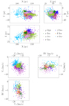 |
Fig. A.1. Distribution of the groups in the representation space. |
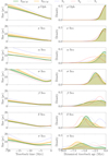 |
Fig. A.2. Dynamical traceback ages. Left panels show the size of each group as a function of traceback time for the different size functions defined in Sect. 4. Right panels show the dynamical traceback ages for the different size functions. |
Comparison with previous studies.
All Tables
All Figures
|
Fig. 1. Top: radial velocity residuals between this work and APOGEE (ΔRV = RV this work – RV APOGEE). The radial velocity measurements that are not compatible within 5σ uncertainties are indicated in red. Bottom: radial velocity distribution of the bona fide sample. We used a Gaussian kernel density with a bandwidth of 0.25 km s−1, similar to the radial velocity precision of the sample. |
| In the text | |
|
Fig. 2. Distribution of the groups in the plane of the sky in Galactic coordinates. The positions of the B-type stars that give their names to the groups are indicated by the white circles. We show the location of the τ Sco star discussed in the main text. The background image shows the emission in radio, at 857 GHz (left, Planck Collaboration I 2020), and in Hα (right, Finkbeiner 2003). |
| In the text | |
|
Fig. 3. Dynamical traceback age distribution obtained for each of the groups using the trace as the size estimator. |
| In the text | |
|
Fig. 4. Colour magnitude diagram of the members of the groups identified in this study. The PARSEC isochrones corresponding to the dynamical traceback ages determined in this study are indicated in red. The PARSEC isochrones at 5 and 20 Myr and the 1 mag extinction vector are also indicated. |
| In the text | |
|
Fig. 5. Orbits back in time of the centre of each of the groups identified in this study. The coloured trajectories indicate the orbit of the groups from the present back to the birth time determined in this study within the reported uncertainties in the dynamical ages. The grey trajectories indicate the orbit of the groups from the birth time determined in this study to 20 Myr ago. |
| In the text | |
|
Fig. 6. Schema representing the proposed star-formation scenario in Upper Scorpius. |
| In the text | |
|
Fig. A.1. Distribution of the groups in the representation space. |
| In the text | |
|
Fig. A.2. Dynamical traceback ages. Left panels show the size of each group as a function of traceback time for the different size functions defined in Sect. 4. Right panels show the dynamical traceback ages for the different size functions. |
| In the text | |
Current usage metrics show cumulative count of Article Views (full-text article views including HTML views, PDF and ePub downloads, according to the available data) and Abstracts Views on Vision4Press platform.
Data correspond to usage on the plateform after 2015. The current usage metrics is available 48-96 hours after online publication and is updated daily on week days.
Initial download of the metrics may take a while.