| Issue |
A&A
Volume 667, November 2022
|
|
|---|---|---|
| Article Number | A93 | |
| Number of page(s) | 10 | |
| Section | Planets and planetary systems | |
| DOI | https://doi.org/10.1051/0004-6361/202244326 | |
| Published online | 17 November 2022 | |
Estimation of the space weathering timescale on (25143) Itokawa: Implications on its rejuvenation process
1
Department of Physics and Astronomy, Seoul National University,
1 Gwanak-ro, Gwanak-gu,
Seoul
08826, Republic of Korea
2
SNU Astronomy Research Center, Department of Physics and Astronomy, Seoul National University,
1 Gwanak-ro, Gwanak-gu,
Seoul
08826, Republic of Korea
e-mail: This email address is being protected from spambots. You need JavaScript enabled to view it.
; This email address is being protected from spambots. You need JavaScript enabled to view it.
Received:
23
June
2022
Accepted:
1
September
2022
Abstract
Context. The space weathering timescales of near-Earth S-type asteroids have been investigated using several approaches (i.e., experiments, sample analyses, and theoretical approaches), yet there are orders of magnitude differences.
Aims. We aim to examine the space weathering timescale on a near-Earth S-type asteroid, Itokawa, using Hayabusa/AMICA images, and further investigate the evolutional process of the asteroid.
Methods. We focused on bright mottles on the boulder surfaces generated via impacts with interplanetary dust particles (IDPs). We compared the bright mottle size distribution with an IDP flux model to determine the space weathering timescale.
Results. We found that the space weathering timescale on Itokawa’s boulder surfaces is 103 yr (in the range of 102–104 yr), which is consistent with the timescales of space weathering by light ions from the solar wind.
Conclusions. From this result, we conclude that Itokawa’s surface has been weathered rapidly in 103 yr but portions of the surface are exposed due to seismic shaking that was triggered by a recent impact, which created the Kamoi crater.
Key words: minor planets / asteroids: individual: (25143) Itokawa / meteorites / meteors / meteoroids / interplanetary medium
© S. Jin and M. Ishiguro 2022
 Open Access article, published by EDP Sciences, under the terms of the Creative Commons Attribution License (https://creativecommons.org/licenses/by/4.0), which permits unrestricted use, distribution, and reproduction in any medium, provided the original work is properly cited.
This article is published in open access under the Subscribe-to-Open model. This email address is being protected from spambots. You need JavaScript enabled to view it. to support open access publication.
1 Introduction
Space weathering denotes any surface modification processes that may change the optical, physical, chemical, or mineralogical properties of the surface of an airless body (Clark et al. 2002). It is caused by solar wind ion implantation and micrometeorite bombardment (Pieters & Noble 2016). The space weathering effect has been observed on lunar rocks, meteorite samples, and asteroids observed by spacecraft and telescopes (Clark et al. 2002). In particular, materials that consist of ordinary chondrites and S-complex asteroids indicate a decrease in albedo (i.e., darkening), a reddening of the visible spectrum (≲0.7 µm), and a shallowing of the ~1 µm absorption band via space weathering (Clark et al. 2002).
Meanwhile, there is a counter-process against space weathering: rejuvenation or resurfacing, which exposes fresh materials beneath weathered surfaces. Several possible mechanisms for asteroidal resurfacing have been suggested by previous studies. First, tidal interactions with terrestrial planets would trigger resurfacing of the asteroid (Binzel et al. 2010). Seismic shaking by nondestructive impacts would induce granular convection that also rejuvenates surfaces (Richardson et al. 2005). Moreover, thermal fatigue, which is caused by diurnal temperature variations, would break boulders and cobbles on the surface, and result in the exposure of fresh materials (Delbo et al. 2014). Furthermore, the Yarkovsky-O’Keefe-Radzievskii-Paddack (YORP) effect accelerates the spin rate and would cause mass shedding and global resurfacing (Pravec & Harris 2007; Graves et al. 2018).
An S-type, near-Earth asteroid, (25143) Itokawa is one of the most evident exhibitions of space weathering and resurfacing phenomena. The unique trait of the asteroid is a large variety of albedos and spectra on its surface, found from the multiband imaging observation by the Asteroid Multiband Imaging CAmera (AMICA) on board the Hayabusa spacecraft (Saito et al. 2006). Previous studies proved that space weathering is the primary cause of albedo and spectral variation. Hiroi et al. (2006) investigated the near-infrared spectrometer (NIRS) data on board the Hayabusa spacecraft and constructed modeled spectra of Itokawa as a mixture of the spectrum of an LL5 chondrite (Alta’meem) and nanophase iron, taking account of the space weathering. Ishiguro et al. (2007) presented a global map of space weathering degrees using AMICA images. More recently, Koga et al. (2018) conducted a principal component analysis on multiband spectra derived from AMICA images and confirmed that the main trend of the spectral variation is consistent with spectral alteration by laboratory simulations of space weathering. Moreover, weathered rims found from the returned samples are regarded as the most definitive evidence for the occurrence of space weathering on the asteroid surface (Noguchi et al. 2014).
It is, however, important to note that the exposure time of Itokawa’s surface material is not well determined, even though the Hayabusa project comprehensively explored the asteroid via remote-sensing observations and laboratory analyses of the returned samples. There is a large discrepancy in the estimate of the surface age up to four orders of magnitude (from 100 to 106 yr, Bonal et al. 2015; Koga et al. 2018; Noguchi et al. 2011; Keller & Berger 2014; Matsumoto et al. 2018; Nagao et al. 2011). In addition, there is still an enormous discrepancy between mechanisms for determining the space weathering timescale of an S-type asteroid. It thus depends on the physical processes that cause the space weathering (108 yr for micrometeorite impacts, Sasaki et al. 2001; 104–106 yr for heavy-ion irradiation, Brunetto et al. 2006; 103–104 yr for H+ and He+ ion irradiation, Hapke 2001 and Loeffler et al. 2009). These discrepancies are major obstacles to understanding the evolutional history of Itokawa’s surface.
We propose a novel idea to estimate Itokawa’s surface age, focusing on bright mottles on the boulder surfaces to alleviate these discrepancies. It was reported that the bright mottles consist of fresh material under the weathered patina of boulders that are exposed by impacts with millimeter- to centimeter-sized interplanetary dust particles (IDPs, Takeuchi et al. 2009, 2010). Because these mottles become obscure due to space weathering, which makes them darker and redder again, the number of observable mottles is controlled by the balance of the timescale of space weathering and the IDP impact frequency. We calculated the occurrence frequency of the bright mottles as a function of size and compared the frequency to the number of the bright mottles to determine the space weathering timescale on Itokawa. Here, we defined the space weathering timescale as the characteristic time needed for changing from fresh ordinary chondrite (OC)-like optical property to the typical (i.e., matured) optical property of Itokawa’s surface. We describe our method in Sect. 2 and we report our findings in Sect. 3. Based on these results, we discuss the possible resurfacing mechanism that results in the large-scale optical heterogeneity in Sect. 4.
2 Methods
In this chapter, we describe data preparation, the bright mottle detection technique, and a model for comparing our observational results with IDP impact flux. The detailed descriptions are shown in the following subsections.
2.1 Data preparation
The Hayabusa spacecraft arrived at the gate position (about 20 km from Itokawa) on 2005, September 12, and shifted to the home position (about 7 km from Itokawa; Fujiwara et al. 2006). During these phases, the mission team investigated the global structures of the asteroid using the onboard instruments. In October 2005, the spacecraft moved to several positions with different solar phase angles and approached closer distances for detailed investigations. The mission team conducted two touchdown rehearsals on 2005, November 4 and 12 (Yano et al. 2006). Finally, the spacecraft landed on Itokawa’s surface on 2005, November 19 (Fujiwara et al. 2006). Figure 1 shows the altitudes of the spacecraft in November 2005. These data were taken using the Light Detection and Ranging instrument (LIDAR; Abe et al. 2006; Mukai et al. 2007). In Fig. 1, we emphasize the altitude at which the AMICA images were obtained with different symbols (the open and filled red circles).
Among the imaging data available at the official website of the DAta Archives and Transmission System (DARTS), the Institute of Space and Astronautical Science (ISAS), and Japan Aerospace Exploration Agency (JAXA)1, we selected five AMICA images (ST_2544540977_v, ST_2544579522_v, ST_2544617921_v, ST_2563511720_v, and ST_2572745988_v) taken on 2005, November 12 and 19 (Fig. 2). These images were taken during the second rehearsal and touchdown. We selected these images because they have good spatial resolutions (< 15 mm pixel−1) and contain large boulders (whose longest axis is longer than 1 m). The resolution and boulder sizes are important factors in detecting small mottles and increasing the reliability of the statistical analysis by the law of large population. We did not use ST_2563537820_v (an open circle on November 19 in Fig. 1) for our analysis because there is no large (> 1 m) boulder in the image despite the high resolution (6.9 mm pixel−1). Detailed information on the images for our analysis is given in Table 1.
We subtracted bias and corrected flat from the raw images following Ishiguro et al. (2010). After the preprocessing, we applied the Lucy-Richardson deconvolution algorithm to improve the blurred resolution of the AMICA images (Richardson 1972; Lucy 1974). The usability of the deconvolution technique is confirmed in Ishiguro et al. (2010).
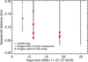 |
Fig. 1 Distance between the spacecraft and Itokawa’s surface. The gray circles denote the data taken by Hayabusa/LIDAR in November 2005 (Mukai et al. 2012). Red (open and filled) circles indicate the distances of the spacecraft when each image was taken at a distance closer than 200 m. Filled red circles show the images examined in this study. |
2.2 Detection of bright mottles from images
Because small boulders tend to be covered by movable regolith particles, bare rock surfaces may not be exposed on the small boulders. For this reason, we selected a total of 12 large boulders (Fig. 2). The longest axis of these boulders is larger than 1m. Assuming that the boulders’ surfaces are perpendicular to the AMICA boresight vector, the total surface area is estimated to be 27.1 m2.
We utilized Source-Extractor2 (Bertin & Arnouts 1996) to detect bright mottles from boulders. It should be noted that there are large-scale brightness fluctuations on a boulder surface due to the different illumination conditions. This inhomogeneity is not common in astronomical images, for which Source-Extractor is mainly designed. Therefore, we flattened the background by subtracting smoothed images made from a two-dimensional median filter (without using the background detection algorithm in Source-Extractor). We applied the two-dimensional median filter with a square width of 19 pixels to the original image. We decided the filter size to flatten the large-scale background (≳10 cm) while leaving small structures of bright mottles (≲ 10 cm). Panels a, b, and c in Fig. 3 are the examples of the original, median-filtered, and background-subtracted images of a boulder, respectively.
Then, we ran Source-Extractor with a 3-sigma detection threshold. This threshold was chosen to distinguish bright mottles from the small-scale fluctuations caused by the Poisson noise and textures of the boulders. On the other hand, the background mesh size for the calculation of background standard deviation was also 19 pixels, the same size as the median filter. The minimum area for the detection was 2 pixels, to avoid false detection due to hot pixels. With this setting, we detected 499 bright sources from 12 boulders. After this detection process, we rejected sources with elongations (the ratio of major to minor axis) larger than 2.5. This criteria was based on Elbeshausen et al. (2013), which showed the elongation of the crater is lower than 2.5, except in extreme impact conditions (impact angle <5 degrees). From this criterion, we filtered out 57 sources (11.4% of detected sources) and determined 442 sources as bright mottles created by impacts with interplanetary dust particles.
We counted the number of pixels above the threshold for each bright mottle and calculated the area covered by these pixels. After that, we converted the area to the diameter of a circle with an equivalent area. Hereafter, we refer to this diameter as the size of the bright mottle. Once we obtained the size, we derived cumulative size-frequency distributions (SFDs) of bright mottles on ten boulders. We employed a logarithmic bin size (Crater Analysis Techniques Working Group et al. 1979). The range and bin size of the crater’s SFDs are given in Table 2.
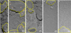 |
Fig. 2 Five images analyzed in this study. The file names are (a) ST_2544540977_v, (b) ST_2544579522_v, (c) ST_2544617921_v, (d) ST_2563511720, and (e) ST_2572745988. We selected twelve large boulders (enclosed by yellow lines) for the analysis. We show enlarged images of the areas surrounded by orange squares in Fig. 6. |
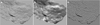 |
Fig. 3 An example of the (a) original, (b) median-filtered, and (c) background-subtracted images used for the analysis. The original image is a part of ST_2544579522_v.fits. |
Images used in this study.
2.3 IDP impact model
As described above, we consider that recent IDP impacts on the bare boulder surface formed bright mottles. Accordingly, if the IDP impact flux is known, it is possible to derive the number of mottles and compare it to the number of detected bright mottles. We utilized the Meteoroid Engineering Model Version 3 (MEM3, Moorhead et al. 2020) model to derive the IDP impact flux colliding with boulder surfaces. This model was developed for the risk assessment of spacecraft navigating in the near-Earth region (the heliocentric distance between 0.2 and 2.0 au). It is also applicable to any celestial bodies if the orbital information is given. We obtained Itokawa’s orbital information from the JPL Horizons Web interface3. This ephemeris includes state vectors of Itokawa with respect to the Earth, starting from 2019, June 10 (JD 2 458 644.5) to 2020, December 16 (JD 2 459 199.5), for 555 days (approximately one orbital period of Itokawa, Fujiwara et al. 2006). We assumed that the flux averaged over one orbital period remained as a constant since the orbit of the asteroid has not been significantly altered for over one million years (Yoshikawa 2002). Because the rotation axis of Itokawa is nearly aligned to the ecliptic south pole ([λ,β] = [128°.5, −89°.66], where λ and β are the ecliptic longitude and latitude of the pole orientation, Demura et al. 2006 and Fujiwara et al. 2006), and the boulders for our analysis distribute near the equatorial region, we employed azimuthally averaged flux. Thus is the impact flux to a target body rotating around the ecliptic pole and averaged along the azimuth direction.
The MEM3 model assumes two meteoroid populations, namely, high- and low-density populations with different mass densities based on Kikwaya et al. (2011). For each population, the MEM3 model calculates the impact flux per square meter per year, H(v), as a function of the impactor velocity v in the mass range of mmin ≤ m ≤ mmax, where mmin = 10−6 g and mmax = 10 g are given, respectively. In Fig. 4, we show H(v) for a target in Itokawa’s orbit, where we specified the velocity interval of ∆v = 1 km s−1 for the calculation.
H(v) is written as
 (1)
(1)
where f(m,v) is a differential impact flux distribution with respect to v and m, per square meter per year. It is important to note that the mass dependency of the impact flux is not available in H(v) because it has an integrated form with respect to m. Accordingly, (m, v) in Eq. (1) is more useful than H(v) for our study because we need to compare the size (derivable from m) frequency distribution of the bright mottles with a model. Following the recommendation in Moorhead et al. (2020), we incorporated the cumulative IDP flux model FGrün(m) in Grün et al. (1985) into H(v) obtained by the MEM3 model. It is given by
 (2)
(2)
where c1 = 2.2 × 10³, c2 = 15, c3 = 1.3 × 10⁻⁹, c4 = 1011, c5 = 1027, c6 = 1.3 × 10⁻¹⁶, c7 = 1.0 × 10⁶, γ1 = 0.306, γ2 = −4.38, γ3 = −0.36, and γ4 = −0.85 are constants. The mass, m, is in the unit of a gram in Eq. (2).
With FGrün(m), the cumulative IDP flux with the particle mass larger than m is given as a function of mass and velocity:
 (3)
(3)
where we chose the denominator (the cumulative flux for m > mmin) to conserve the total flux. Because the MEM3 model generates the flux for discrete velocity and mass density (see below) values, we hereafter notate discrete values as (mi, vj,δk) rather than (m, v, δ) for mass, velocity, and mass density. Table 2 summarizes the notation and the range of these discrete physical quantities. For our convenience, we converted the cumulative flux FGrün(mi) into the differential flux within ith mass bin as below:
 (4)
(4)
The MEM3 model also provides a probability distribution of the mass density δk. The probability distribution function, C(δk), is defined as the ratio of the number of particles within a given density bin to the total number of particles. In the MEM3 model, C(δk) is independent of mi and vj. With this function, the IDP flux for a given mass, velocity, and mass density is calculated from
 (5)
(5)
Next, we considered the crater size generated by an IDP impact with a given mi, vj, and δk. We utilized the crater size model in Holsapple (1993). We thus calculated the cratering volume  excavated by an impact with a given mean mass
  , mean velocity
  , and mass density
  by following equations:
 (6)
(6)
where πV is the so-called cratering efficiency, defined as a ratio of the crater mass to the impactor mass (Holsapple 1993).  and
and  denote the mean radius and the normal component of the mean velocity of the impactor, respectively. We assumed an oblique impact with the most probable impact angle θ = 45° (Gault & Wedekind 1978). This assumption of the oblique impact reduces the vertical impact velocity by a factor of
  (i.e.,
  ). The constants, Y, ρ, and g are the tensile strength, the bulk density, and the surface gravity of the target body, respectively. We assumed a spherical impactor whose mean radius is given as:
 (7)
(7)
To obtain the crater volume  , we used Eqs. (6)-(7) for impactors with given
  , and
, and  . We substituted ρ = 3.4 g cm−3 based on the measurement of the bulk density of Itokawa’s samples (Tsuchiyama et al. 2011). The gravitational acceleration on Itokawa’s surface is given as g = 8.4 × 10⁻³ cm s−2 (Tancredi et al. 2015). For the other parameters that characterize the target boulders, we assumed a hard rock-type material and referred to the values in Holsapple (1993, 2022). Table 3 summarizes the applied values for the computation. With Eq. (6), we calculated πV for each impactor with a given
  , and
, and  , and obtained the crater mass ρV. The crater radii were then derived as R = KrV1/3, in the case of a simple bowl-shaped crater (Holsapple 2022).
Holsapple & Housen (2013) asserted that craters on small (sub-kilometer sized) asteroids are expected to be spall craters. They are a kind of crater surrounded by shallow spallation features, with diameters two to four times larger than those of simple bowl-shaped craters. Since the depth of the space weathered rim layer found in Itokawa samples is thin enough (<1 µm, Noguchi et al. 2014), it is reasonable to assume that the diameters of bright mottles are equivalent to the diameters of the bowl-shaped craters. Therefore, the diameter of bright mottles including spalled region can be given as D = 2CspallR (2 ≤ Cspall ≤ 4). We discuss the effect of Cspall in Sect. 4.2.5.
After deriving D, we counted the total number of craters within the given diameter bins, N(Dl). For the consideration of the diameter bins, we employed a logarithmic bin size to match the bright mottle SFD from the observation, namely,
 (8)
(8)
Then, the number of craters within l-th diameter bin, N(Dl) was counted as
 (9)
(9)
where the subscript l is an ordinal number up to 50 (i.e., l = 1, 2,…, 50).
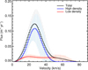 |
Fig. 4 Cumulative IDP flux averaged over one orbital revolution of Itokawa around the Sun. The error bars correspond to the range of the IDP flux during one orbit revolution. |
Parameters used for the evaluation of the crater’s diameter.
3 Results
We identified 442 bright mottles from twelve boulders (with a projected total area of 27.1 m2). The average spatial density is 16.3 m−2. We present our findings in the following sections.
3.1 Cumulative size-frequency distributions
Figure 5 indicates the cumulative size-frequency distributions (CSFDs) of bright mottles per unit area on each boulder. Panels a-e in Fig. 5 were obtained from different images (i.e., the different spatial resolutions), while the different markers in each panel are CSFDs on each boulder, and Fig. 5f shows the average of all 12 boulders. At first glance, the slopes and absolute numbers of CSFDs match one another within an order of magnitude, regardless of the different images or different boulders. From this evidence, it is expected that the exposure time of each boulder is similar to the exposure times of the others. For all profiles, slopes of CSFDs for larger bright mottles are steeper than those for smaller ones. This is because the spatial resolution is insufficient to detect and measure small mottles with diameters equivalent to the pixel resolutions. The inflection points (D ~ 3-4 cm) in panel a of Fig. 5 is larger than the inflection points (D ~ 2–3 cm) in panels b and c due to the different spatial resolutions of each image, indicating that the inflection points are determined by artifacts of the observational resolutions.
Figure 5 also compares observed CSFDs with the IDP impact model (see, Sect. 2.3). The slopes of the CSFDs are consistent between these observations and the IDP impact model. For the large bright mottles (3–7 cm) in panel f of Fig. 5, the power index of CSFDs is q = −3.67 ± 0.23, where the error stands for the standard deviation of the CSFDs of different boulders. The observed power index is consistent with the IDP impact model (i.e., q = −3.61 ± 0.03) within the error ranges. In each figure, we multiplied the modeled impact flux by several different exposure times to space (102, 103, 104, 105, and 106 yr). Ignoring the observed CSFDs in the small size range, we found that the observed CSFDs match the IDP CSFDs with the exposure time of ~1000 yr. Accordingly, we conclude that impact-triggered bright mottles have been obscured by the space weathering effect, which has changed the reflectance of the bright mottles, becoming as dark as the surrounding areas in a timescale of 1000 yr.
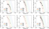 |
Fig. 5 CSFDs of bright mottles per unit area (black diamonds) compared to the estimated CSFD from the IDP impact models (colored lines). Error bars indicate a 1-σ confidence interval, which assumes a Poisson distribution. Panels with the labels a–e are obtained from different images (ST_2544540977, ST_2544579522, ST_2544617921, ST_2563511720, and ST_2572745988) and the panel with label f shows the average of the five images listed above. |
3.2 The morphology
As mentioned above, we estimated the space weathering timescale assuming that bright mottles are impact craters with pit-halo structures. The pit-halos have a rounded central pit surrounded by a region of partially excavated material. To confirm the existence of the pit-halo structures, we examined the morphology. Figure 6 shows enlarged images of the largest bright mottles. Because the largest bright mottle (Fig. 6a) has a diameter of 8 pixels (5 cm), it is possible to confirm the detailed shapes for large bright mottles. We identified at least three halo features (Figs. 6a, d, and e) enclosed the central holes. The pit-halo features are unclear for the mottles smaller than ~3 cm because of the insufficient image resolution. The diameter ratio between the central depression (the dark parts in the center) to the surrounding halo is ~2.8 by visual inspection, which is in accordance with the general value for pit-halo craters (Holsapple & Housen 2013). For this reason, all detected bright mottles are likely accompanied by pit-halo structures.
4 Discussion
We compare our results with previous research in Sect. 4.1 and discuss the uncertainties of our approach for deriving the space weathering timescale (TSW) in Sect. 4.2. Lastly, we consider a possible phenomenon that might have occurred on Itokawa’s surface in about the past ~103 yr, based on the derived TSW, in Sect. 4.3.
4.1 Comparison with previous research
TSW has been investigated using laboratory experiments and theoretical approaches. In early studies of space weathering, Yamada et al. (1999) and Sasaki et al. (2001) conducted irradiation in a space weathering simulation for the micrometeorite impacts. Sasaki et al. (2001) found that the spectrum of olivine pallet samples indicated a spectrum consistent with Atype asteroids (olivine-rich S-type) after 30-mJ irradiation of the laser. From this experiment, they derived TSW = 108 yr in the case of space weathering by dust impact heating (Sasaki et al. 2001).
On the other hand, Loeffler et al. (2009) investigated the solar wind’s influence by conducting a He+ ion irradiation experiment on their olivine samples and they applied their experimental result to objects at 1 au. They found that the characteristic TSW induced by the solar wind He+ ion irradiation is TSW = (5–1.3) × 103 yr. Hapke (2001) also estimated that the space weathering time required to alter asteroid soil by Hydrogen ions is about 5 × 10⁴ yr at 3 au. Assuming that the darkening time is inversely proportional to the solar wind flux, we derived TSW = 8 × 10³ yr on Itokawa’s orbit (the semimajor axis a = 1.32 au and the eccentricity e = 0.28) from this Hapke’s estimate for H+ ion irradiation.
The space weathering time caused by heavy ion irradiation was also examined. Strazzulla et al. (2005) investigated the spectral alteration of an OC meteorite (H5) by irradiating with Ar2+ to simulate heavy ion irradiation in the solar wind and estimated TSW = 1.3 × 10⁶ yr for S-type near-Earth asteroids (including Itokawa). Considering elements heavier than argon, Strazzulla et al. (2005) further found that TSW by heavy elements is on the order of 104–106 yr for S-type near-Earth asteroids. Brunetto & Strazzulla (2005) performed ion irradiation experiments using four different ions (H+, He+, Ar+, and Ar2+) and derived TSW < 106 yr.
Comparing these experimental results, our observational research of bright mottles is consistent with the estimate by the light-element (He+ and H+) experiments and close to the lower-end estimate by the heavy elements. However, it is about five orders of magnitude shorter than the estimate of dust impact heating.
Conclusive evidence of space weathering (i.e., nanophase iron) by solar wind ions was found in samples from Itokawa (Noguchi et al. 2011). In addition, noble gas elements (He, Ne, and Ar) from the Sun trapped in various depths of Itokawa’s samples were also detected. Keller & Berger (2014) used solar flare track density to date regolith samples to 102–104 yr. Matsumoto et al. (2018) compared the size distribution of microcraters on the surface of the Itokawa sample and the lunar secondary impact fluxes, and estimated the direct exposure timescale of Itokawa regolith particles as 102–103 yr. Nagao et al. (2011) estimated the space weathering ages of Itokawa samples to be 150–550 yr based on an analysis of He concentration in the samples. Our estimate of the space weathering timescale is also consistent with the exposure time of the regolith particles.
Itokawa’s surface age has also been determined from remote-sensing observation data (105–106 yr, Bonal et al. 2015; Koga et al. 2018). However, as already pointed out in Bonal et al. (2015) and Tatsumi & Sugita (2018), the estimate changes by one or two orders of magnitude depending on the experimental data used to convert spectra and colors to ages. Therefore, it is safe to say that our result does not contradict previous measurements using the remote-sensing data.
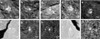 |
Fig. 6 Close-up images of the largest bright mottles. Labels in each panel correspond to the areas in Fig. 2b. |
4.2 Uncertainty analysis
We estimated the space weathering timescale to be 1000 yr based on the CSFDs of bright mottles compared with the IDP impact model. It is important to scrutinize problems hidden behind our analysis, the model, and assumptions, and clarify the uncertainty of the estimated space weathering timescale to assess the confidence in the result. Uncertainties related to our analysis, measurements, and assumptions include: (i) uncertainty in the mottle counting, (ii) possibility of the false detection, (iii) uncertainty of the crater size measurement, (iv) uncertainty of the MEM3 IDP impact model, and (v) uncertainty for converting from crater size to impactor size.
In the following subsections (Sects. 4.2.1-4.2.5), we discuss these uncertainties and examine the impact on our result.
4.2.1 Uncertainty in the mottle counting
We set a 3-sigma threshold for the mottle detection and counting. This threshold may underestimate the number of mottles because there would be fainter mottles under the detection limit. We consider how sensitive our mottle detection algorithm is for space weathering research. We made the following estimate based on the radiance factor, RADF, in panel b of Fig. 2. We converted the observed counts, I(x, y), into radiance factor using the equation below:
 (10)
(10)
where C0 and texp are the calibration factor (for v-band data, 3.42 ± 0.10 × 10⁻³ (W m−2 µm−1 sr−1)/(DN s−1), Ishiguro et al. 2010) and the exposure time, respectively. x and y denote the pixel coordinates on the AMICA images. Sv is the solar irradiance in v-band at the heliocentric distance of r in au4. With Eq. (10), we found that the average RADF value and the 3-sigma detection threshold are 0.193 and 0.208, respectively. Our detection algorithm cannot extract mottles if they are fainter than RADF = 0.208 (8% excess of the ambient weathered region).
The albedo of an OC is expected to decline precipitously in the early stages of space weathering evolution and reach a constant value when the abundance of nanophase irons saturates in the rims of OC materials. Shestopalov et al. (2013) investigated the time evolution of albedos for OCs (including LL6, an analog of Itokawa) and suggested that the albedo dropped from 0.17–0.52 to ≈0.05 in the early stage, and reached a nearly constant value. Although the definition of the albedo is not described explicitly in Shestopalov et al. (2013), it seems to us that it is the Bond albedo because they compared the albedo with meteorite spectra in Gaffey (1976), where the spectral data are comparable to the Bond albedo. From the low Bond albedos of Itokawa (0.02 ± 0.01, Lederer et al. 2008), most of the Itokawa surface material is likely weathered to some degree, not fresh material. Moreover, because the 3-sigma detection limit of our algorithm captures an 8% albedo excess (significantly smaller than the initial drop in albedo), we think the detection capability of the bright mottles is high enough to characterize the initial precipitous darkening phase by the space weathering. While there can be faint mottles under our detection limit, we consider that they were almost saturated by the initial space weathering effect and indicated a slow albedo decrease in the matured phase.
4.2.2 Possibility of the false detection
We anticipate some objections to our assumption of the pit-halo crater because most of the bright mottles are not resolved in the AMICA images. Accordingly, some detected mottles may not be pit-halo craters but bright inclusions. For instance, chondrules with a large reflectance might be exposed on the surface and mistakenly recognized as pit-halo craters. However, we would argue that such a false counting of the bright inclusions is less likely because the typical chondrule size in LL-type OCs is ~1 mm on average (up to 3.5 mm), even smaller than the detected bright mottles (Friedrich et al. 2015). Moreover, the consistency in the slopes of the CSFDs between our IDP impact model and the detected mottles implies that the detected bright mottles are likely the impact origin. The pit-halo structure and quasi-circular morphology found in the close-up images of large mottles (see Fig. 5) also supports the assumption of the impact origin. For these reasons, we would assert that the influence of false detections can be negligible, especially in the large size range.
4.2.3 Uncertainty of the crater size measurement
The diameters of bright mottles are determined from the observed images. Thanks to the image deconvolution technique, the image resolutions are comparable to the pixel resolutions (i.e., 6–11 mm pixel−1). The resolutions are sufficient to derive the sizes of the large mottles (D = 3–5 cm, 5–8 pixels) with an accuracy of ≈10–20%. However, as we mentioned in Sect. 3.1, the derived diameter would be less accurate for the small mottles (diameter <3 cm). In fact, the CSFDs do not match the IDP impact model in this small size range (<2–3 cm), probably because of the lack of image resolutions.
To summarize our discussion so far (Sects. 4.2.2-4.2.3), we can assert that our estimate of the space weathering timescale is sufficiently reliable because we focused on CSFDs with a reliable size range (>3 cm).
4.2.4 Uncertainty of the IDP flux model
Moorhead et al. (2020) compared the MEM3 IDP flux model with in situ measurements. They converted collision records from Pegasus satellites and the Long Duration Exposure Facility (LDEF) into flux using ballistic limit equations. They found that the impact rate predicted by the MEM3 model is two to three times lower than the Pegasus measurement. On the contrary, the MEM3 model indicated the impact rate two times as high as the LDEF observation. Moorhead et al. (2020) interpreted that these discrepancies are within a predicted range because the inherent uncertainty of Grün’s model (the underlying model for MEM3) near 1 au is a factor of roughly three of the nominal flux (Drolshagen 2009). Therefore, the space weathering timescale also has a factor of three uncertainty associated with the MEM3 IDP flux model.
4.2.5 Crater size relation and spallation
We employed Holsapple’s scaling law to derive the diameter of the bright mottles produced by IDP impacts (Sect. 2.3). Although this Holsapple’s scaling law has been widely used, it is worthwhile testing differences in crater diameters using a different model.
Furthermore, Suzuki’s group performed impact experiments on porous targets. Suzuki et al. (2021) conducted oblique impact experiments on a porous target and found that the pit-halo structure disappeared. Although we have assumed in this paper that Itokawa boulders have low porosity, it is important to consider the possibility of boulders with high porosity. However, it is unlikely that the boulders we analyzed are as porous as those in the oblique impact experiment of Suzuki et al. (2021) because the pit-halo craters are found on the boulders. In addition, the low porosity of LL chondrites and the Itokawa samples (0h3@10% with an average of 1.5 and 1.9%, respectively) may also support our argument for low porosity (Tanbakouei et al. 2019).
Moreover, there is an ambiguity in the model associated with the diameter ratio of pit-halo craters to bowl craters. It is between two and four (Holsapple & Housen 2013). We adopted only the intermediate value three in Sect. 2.3. Varying this ratio of two (lower limit) and four (upper limit), we find that the space weathering timescale changes by a factor of about four and 0.35, respectively.
Table 4 summarizes the major uncertainty factors, and the upper and lower limits of the space weathering timescales. Even with all these uncertainties, the error in our estimate of the space weathering timescale is likely to be smaller than an order of magnitude.
Upper and lower limits of the space weathering timescale for each uncertain factor.
4.3 Implications on the resurfacing mechanism
The space weathering timescale estimated in this study provides important information on the evolution of Itokawa. In particular, we focus on the ubiquity of fresh regions throughout Itokawa’s surface. It is interesting to consider how fresh surfaces are exposed despite the short timescale of space weathering (~ 1000 yr). In this section, we consider the possible mechanisms for exposing fresh surfaces.
Tidal resurfacing might have triggered a large-scale exposure of fresh materials (Binzel et al. 2010). However, Binzel et al. (2010) suggested that Q-type asteroids underwent close encounters with terrestrial planets within the last 5 × 10⁵ yr, longer than the space weathering timescale derived from this study. Besides, Yoshikawa (2002) reported that Itokawa has maintained its present orbit for several thousand years, or even much longer, suggesting that it is unlikely that it encountered a planet over the space weathering timescale. Thermal fatigue caused by a diurnal temperature gradient would have also created fresh materials by destructing the surface materials (Delbo et al. 2014). Ravaji et al. (2018) suggested that the lifetime of 10cm boulders on the surface of an S-type asteroid with a rotation period of 12 h is 103–104 yr, comparable to the space weathering timescale of 103 yr. This effect may be efficient near the equatorial region where the diurnal temperature variation is maximum. However, from the remote-sensing observations, fresh materials are not related to the latitude, but rather the geological features such as steep slopes and crater rims.
Acceleration of rotation by the YORP effect would also cause mass shedding to expose unweathered subsurfaces (Pravec & Harris 2007; Graves et al. 2018). Lowry et al. (2014) found the rotation of Itokawa has been accelerated by 45 ms yr−1 during monitoring observations from 2001 to 2013. Hence, it is unlikely that rejuvenation is caused by mass losses due to faster rotation in the past. Granular convection from impact-induced, global seismic shaking would expose unweathered grains on the asteroidal surface. However, this process is also unlikely to be a major resurfacing process because Shestopalov et al. (2013) show that this process only decelerates and does not counteract the space weathering. Moreover, Yamada et al. (2016) estimate that the granular convection timescale for Itokawa is the order of 107 yr, four orders larger than our space weathering timescale.
The remaining cause is a single impact. It is reported that the Kamoi crater (a diameter of 8 m) is the freshest terrain on Itokawa (Ishiguro et al. 2007). Assuming an oblique impact (45-degree incident angle) of an S-type impactor on Itokawa (the 0.33 km-sized S-type target asteroid), we find that a 6.5 cm-sized impactor (431 g) creates the Kamoi crater based on the Holsapple model (Holsapple 2022). This size estimate is consistent with (Tatsumi & Sugita 2018; 20 cm) within around a factor of three uncertainty. We further estimate that the impact flux on the Itokawa-sized object at 1 au is 10−5 yr−1 for this range of size and mass (6.5 cm and 431 g) using Grün’s interplanetary dust flux model (Grün et al. 1985). Accordingly, the impact event that created the Kamoi crater is extremely rare, occurring only once every 105 yr. Although the frequency is low, we suspect that the impact that created the Kamoi crater and the subsequent rejuvenation process by seismic shaking is a possible scenario for explaining the ubiquitous exposure of fresh surfaces. The impact energy is large enough to cause global seismic shaking, and induce granular convection and boulder movements on the surface (Miyamoto 2014).
Recently, Hasegawa et al. (2022) reported a spectral change of (596) Scheila as exposure of fresh surface by a large impact event in 2010. Although the spectral types are different between Itokawa (S-type) and (596) Scheila (D-type), such time-domain studies of space weathering are becoming possible. We anticipate that further experimental and observational studies of the degree of space weathering progression will be conducted.
5 Conclusions
In this paper, we have introduced a new technique using size-frequency distributions of bright mottles at the surface of boulders to estimate the space weathering timescale of the asteroid Itokawa. We suggest that the time required to alter materials with pristine state into a similar degree of the space weathering of the average Itokawa surface is 103 yr, with an order of magnitude uncertainty. This result is consistent with the laboratory simulation of space weathering using Hydrogen and Helium ions, the most abundant species within the solar wind. Based on our result, we conjecture that a single impact on the Kamoi crater and the subsequent seismic shaking produced the ubiquitous exposure of Itokawa’s fresh surfaces.
Acknowledgements
We deeply appreciate Sasaki Sho and Emmanuel Lellouch for the valuable opinions and suggestions as a reviewer and an editor, respectively. We also thank Keith A. Holsapple and Akiko M. Nakamura (Kobe University) for helpful comments on the impact modeling of interplanetary dust particles. This work at Seoul National University was supported by the National Research Foundation of Korea (NRF) funded by the Korean government (MEST; No. 2018R1D1A1A09084105). S.J. was supported by the Global Ph.D. Fellowship Program through a National Research Foundation of Korea (NRF) grant funded by the Korean Government (NRF-2019H1A2A1074796).
References
- Abe, S., Mukai, T., Hirata, N., et al. 2006, Science, 312, 1344 [NASA ADS] [CrossRef] [Google Scholar]
- Bertin, E., & Arnouts, S. 1996, A&AS, 117, 393 [NASA ADS] [CrossRef] [EDP Sciences] [Google Scholar]
- Binzel, R. P., Morbidelli, A., Merouane, S., et al. 2010, Nature, 463, 331 [NASA ADS] [CrossRef] [Google Scholar]
- Bonal, L., Brunetto, R., Beck, P., et al. 2015, Meteor. Planet. Sci., 50, 1562 [NASA ADS] [CrossRef] [Google Scholar]
- Brunetto, R., & Strazzulla, G. 2005, Icarus, 179, 265 [NASA ADS] [CrossRef] [Google Scholar]
- Brunetto, R., Vernazza, P., Marchi, S., et al. 2006, Icarus, 184, 327 [CrossRef] [Google Scholar]
- Clark, B. E., Hapke, B., Pieters, C., & Britt, D. 2002, Asteroid Space Weathering and Regolith Evolution (Tucson: University of Arizona Press), 585 [Google Scholar]
- Crater Analysis Techniques Working Group, (Arvidson, R. E. et al.) 1979, Icarus, 37, 467 [NASA ADS] [CrossRef] [Google Scholar]
- Delbo, M., Libourel, G., Wilkerson, J., et al. 2014, Nature, 508, 233 [Google Scholar]
- Demura, H., Kobayashi, S., Nemoto, E., et al. 2006, Science, 312, 1347 [NASA ADS] [CrossRef] [Google Scholar]
- Drolshagen, G. 2009, Inter-Agency Space Debris Coordination Committee, 1 Elbeshausen, D., Wünnemann, K., & Collins, G. S. 2013, J. Geophys. Res. Planets, 118, 2295 [Google Scholar]
- Friedrich, J. M., Weisberg, M. K., Ebel, D. S., et al. 2015, Chemie der Erde / Geochemistry, 75, 419 [CrossRef] [Google Scholar]
- Fujiwara, A., Kawaguchi, J., Yeomans, D. K., et al. 2006, Science, 312, 1330 [NASA ADS] [CrossRef] [Google Scholar]
- Gaffey, M. J. 1976, J. Geophys. Res., 81, 905Gault, D. E. 1973, Moon, 6, 32 [Google Scholar]
- Gault, D. E., & Wedekind, J. A. 1978, in Lunar and Planetary Science Conference, 374 [Google Scholar]
- Graves, K. J., Minton, D. A., Hirabayashi, M., DeMeo, F. E., & Carry, B. 2018, Icarus, 304, 162 [CrossRef] [Google Scholar]
- Grün, E., Zook, H. A., Fechtig, H., & Giese, R. H. 1985, Icarus, 62, 244 [NASA ADS] [CrossRef] [Google Scholar]
- Hapke, B. 2001, J. Geophys. Res., 106, 10039 [NASA ADS] [CrossRef] [Google Scholar]
- Hasegawa, S., Marsset, M., DeMeo, F. E., et al. 2022, ApJ, 924, L9 [NASA ADS] [CrossRef] [Google Scholar]
- Hiroi, T., Abe, M., Kitazato, K., et al. 2006, Nature, 443, 56 [CrossRef] [Google Scholar]
- Holsapple, K. A. 1993, Ann. Rev. Earth Planet. Sci., 21, 333 [CrossRef] [Google Scholar]
- Holsapple, K. A. 2022, ArXiv e-prints [arXiv:2203.07476] [Google Scholar]
- Holsapple, K. A., & Housen, K. R. 2013, in Lunar and Planetary Science Conference, 2733 [Google Scholar]
- Ishiguro, M., Hiroi, T., Tholen, D. J., et al. 2007, Meteor. Planet. Sci., 42, 1791 [NASA ADS] [CrossRef] [Google Scholar]
- Ishiguro, M., Nakamura, R., Tholen, D. J., et al. 2010, Icarus, 207, 714 [NASA ADS] [CrossRef] [Google Scholar]
- Keller, L. P., & Berger, E. L. 2014, Earth Planets Space, 66, 71 [NASA ADS] [CrossRef] [Google Scholar]
- Kikwaya, J. B., Campbell-Brown, M., & Brown, P. G. 2011, A&A, 530, A113 [NASA ADS] [CrossRef] [EDP Sciences] [Google Scholar]
- Koga, S. C., Sugita, S., Kamata, S., et al. 2018, Icarus, 299, 386 [CrossRef] [Google Scholar]
- Lederer, S. M., Domingue, D. L., Thomas-Osip, J. E., et al. 2008, Earth Planets Space, 60, 49 [NASA ADS] [CrossRef] [Google Scholar]
- Loeffler, M. J., Dukes, C. A., & Baragiola, R. A. 2009, J. Geophys. Res. Planets, 114, E03003 [CrossRef] [Google Scholar]
- Lowry, S. C., Weissman, P.R., Duddy, S. R., et al. 2014, A&A, 562, A48 [NASA ADS] [CrossRef] [EDP Sciences] [Google Scholar]
- Lucy, L. B. 1974, AJ, 79, 745 [Google Scholar]
- Matsumoto, T., Hasegawa, S., Nakao, S., Sakai, M., & Yurimoto, H. 2018, Icarus, 303, 22 [NASA ADS] [CrossRef] [Google Scholar]
- Miyamoto, H. 2014, Planet. Space Sci., 95, 94 [NASA ADS] [CrossRef] [Google Scholar]
- Moorhead, A. V., Kingery, A., & Ehlert, S. 2020, J. Spacecraft Rockets, 57, 160 [Google Scholar]
- Mukai, T., Abe, S., Hirata, N., et al. 2007, Adv. Space Res, 40, 187 [NASA ADS] [CrossRef] [Google Scholar]
- Mukai, T., Abe, S., Barnouin, O., Cheng, A., & Kahn, E. 2012, NASA Planetary Data System, HAY-A-LIDAR-3-HAYLIDAR-V2.0 [Google Scholar]
- Nagao, K., Okazaki, R., Nakamura, T., et al. 2011, Science, 333, 1128 [NASA ADS] [CrossRef] [Google Scholar]
- Noguchi, T., Nakamura, T., Kimura, M., et al. 2011, Science, 333, 1121 [NASA ADS] [CrossRef] [Google Scholar]
- Noguchi, T., Kimura, M., Hashimoto, T., et al. 2014, Meteor. Planet. Sci., 49, 188 [CrossRef] [Google Scholar]
- Pieters, C. M., & Noble, S. K. 2016, J. Geophys. Res. Planets, 121, 1865 [CrossRef] [Google Scholar]
- Pravec, P., & Harris, A. W. 2007, Icarus, 190, 250 [CrossRef] [Google Scholar]
- Ravaji, B., Ali-Lagoa, V., Delbo, M., & Wilkerson, J. W. 2018, in 49th Annual Lunar and Planetary Science Conference, 2628 [Google Scholar]
- Richardson, W. H. 1972, J. Opt. Soc. Am. 62, 55 [NASA ADS] [CrossRef] [Google Scholar]
- Richardson, J. E., Melosh, H. J., Greenberg, R. J., & O’Brien, D. P. 2005, Icarus, 179, 325 [NASA ADS] [CrossRef] [Google Scholar]
- Saito, J., Miyamoto, H., Nakamura, R., et al. 2006, Science, 312, 1341 [NASA ADS] [CrossRef] [Google Scholar]
- Sasaki, S., Nakamura, K., Hamabe, Y., Kurahashi, E., & Hiroi, T. 2001, Nature, 410, 555 [NASA ADS] [CrossRef] [Google Scholar]
- Shestopalov, D. I., Golubeva, L. F., & Cloutis, E. A. 2013, Icarus, 225, 781 [NASA ADS] [CrossRef] [Google Scholar]
- Strazzulla, G., Dotto, E., Binzel, R., et al. 2005, Icarus, 174, 31 [CrossRef] [Google Scholar]
- Suzuki, A., Hakura, S., Hamura, T., et al. 2012, J. Geophys. Res. Planets, 117, E08012 [Google Scholar]
- Suzuki, A. I., Fujita, Y., Harada, S., et al. 2021, Planet. Space Sci., 195, 105141 [NASA ADS] [CrossRef] [Google Scholar]
- Takeuchi, H., Miyamoto, H., & Oku, M. 2009, in Lunar and Planetary Science Conference, 1566 [Google Scholar]
- Takeuchi, H., Miyamoto, H., & Maruyama, S. 2010, in Lunar and Planetary Science Conference, 1578 [Google Scholar]
- Tanbakouei, S., Trigo-Rodríguez, J. M., Sort, J., et al. 2019, A&A, 629, A119 [NASA ADS] [CrossRef] [EDP Sciences] [Google Scholar]
- Tancredi, G., Roland, S., & Bruzzone, S. 2015, Icarus, 247, 279 [NASA ADS] [CrossRef] [Google Scholar]
- Tatsumi, E., & Sugita, S. 2018, Icarus, 300, 227 [NASA ADS] [CrossRef] [Google Scholar]
- Tsuchiyama, A., Uesugi, M., Matsushima, T., et al. 2011, Science, 333, 1125 [NASA ADS] [CrossRef] [Google Scholar]
- Yamada, M., Sasaki, S., Nagahara, H., et al. 1999, Earth Planets Space, 51, 1265 [Google Scholar]
- Yamada, T. M., Ando, K., Morota, T., & Katsuragi, H. 2016, Icarus, 272, 165 [NASA ADS] [CrossRef] [Google Scholar]
- Yano, H., Kubota, T., Miyamoto, H., et al. 2006, Science, 312, 1350 [NASA ADS] [CrossRef] [Google Scholar]
- Yoshikawa, M. 2002, ESA SP, 500, 331 [NASA ADS] [Google Scholar]
All Tables
Upper and lower limits of the space weathering timescale for each uncertain factor.
All Figures
|
Fig. 1 Distance between the spacecraft and Itokawa’s surface. The gray circles denote the data taken by Hayabusa/LIDAR in November 2005 (Mukai et al. 2012). Red (open and filled) circles indicate the distances of the spacecraft when each image was taken at a distance closer than 200 m. Filled red circles show the images examined in this study. |
| In the text | |
|
Fig. 2 Five images analyzed in this study. The file names are (a) ST_2544540977_v, (b) ST_2544579522_v, (c) ST_2544617921_v, (d) ST_2563511720, and (e) ST_2572745988. We selected twelve large boulders (enclosed by yellow lines) for the analysis. We show enlarged images of the areas surrounded by orange squares in Fig. 6. |
| In the text | |
|
Fig. 3 An example of the (a) original, (b) median-filtered, and (c) background-subtracted images used for the analysis. The original image is a part of ST_2544579522_v.fits. |
| In the text | |
|
Fig. 4 Cumulative IDP flux averaged over one orbital revolution of Itokawa around the Sun. The error bars correspond to the range of the IDP flux during one orbit revolution. |
| In the text | |
|
Fig. 5 CSFDs of bright mottles per unit area (black diamonds) compared to the estimated CSFD from the IDP impact models (colored lines). Error bars indicate a 1-σ confidence interval, which assumes a Poisson distribution. Panels with the labels a–e are obtained from different images (ST_2544540977, ST_2544579522, ST_2544617921, ST_2563511720, and ST_2572745988) and the panel with label f shows the average of the five images listed above. |
| In the text | |
|
Fig. 6 Close-up images of the largest bright mottles. Labels in each panel correspond to the areas in Fig. 2b. |
| In the text | |
Current usage metrics show cumulative count of Article Views (full-text article views including HTML views, PDF and ePub downloads, according to the available data) and Abstracts Views on Vision4Press platform.
Data correspond to usage on the plateform after 2015. The current usage metrics is available 48-96 hours after online publication and is updated daily on week days.
Initial download of the metrics may take a while.