| Issue |
A&A
Volume 647, March 2021
|
|
|---|---|---|
| Article Number | A43 | |
| Number of page(s) | 8 | |
| Section | Planets and planetary systems | |
| DOI | https://doi.org/10.1051/0004-6361/202039777 | |
| Published online | 04 March 2021 | |
Size of particles ejected from an artificial impact crater on asteroid 162173 Ryugu
1
Planetary Exploration Research Center, Chiba Institute of Technology,
Narashino
275-0016,
Japan
e-mail: This email address is being protected from spambots. You need JavaScript enabled to view it.
2
Department of Planetology, Kobe University,
Kobe
657-8501, Japan
3
Institute of Space and Astronautical Science, Japan Aerospace Exploration Agency,
Sagamihara
252-5210, Japan
4
JAXA Space Exploration Center, Japan Aerospace Exploration Agency,
Sagamihara
252-5210, Japan
5
Department of Science and Technology, Kochi University,
Kochi
780-8520, Japan
6
Department of Basic Sciences, University of Occupational and Environmental Health,
Kitakyusyu
807-8555, Japan
7
Department of Physics, Rikkyo University,
Tokyo
171-8501, Japan
8
Aichi Toho University,
Nagoya
465-8515, Japan
9
School of Computer Science and Engineering, The University of Aizu,
Aizu-Wakamatsu
965-8580, Japan
Received:
28
October
2020
Accepted:
26
January
2021
Abstract
A projectile accelerated by the Hayabusa2 Small Carry-on Impactor successfully produced an artificial impact crater with a final apparent diameter of 14.5 ± 0.8 m on the surface of the near-Earth asteroid 162173 Ryugu on April 5, 2019. At the time of cratering, Deployable Camera 3 took clear time-lapse images of the ejecta curtain, an assemblage of ejected particles forming a curtain-like structure emerging from the crater. Focusing on the optical depth of the ejecta curtain and comparing it with a theoretical model, we infer the size of the ejecta particles. As a result, the typical size of the ejecta particles is estimated to be several centimeters to decimeters, although it slightly depends on the assumed size distribution. Since the ejecta particles are expected to come from a depth down to ~1 m, our result suggests that the subsurface layer of Ryugu is composed of relatively small particles compared to the uppermost layer on which we observe many meter-sized boulders. Our result also suggests a deficit of particles of less than ~1 mm in the subsurface layer. These findings will play a key role in revealing the formation and surface evolution process of Ryugu and other small Solar System bodies.
Key words: methods: data analysis / methods: observational / minor planets, asteroids: individual: Ryugu / space vehicles: instruments
© K. Wada et al. 2021
 Open Access article, published by EDP Sciences, under the terms of the Creative Commons Attribution License (https://creativecommons.org/licenses/by/4.0), which permits unrestricted use, distribution, and reproduction in any medium, provided the original work is properly cited.
1 Introduction
Particle size distributions on and inside small Solar System bodies reflect the evolution of their surfaces and the physical processes on the bodies. For example, the typical particle size of ~70 μm in the lunar regolith is attributed to a result of impact processes on the lunar surface (McKay et al. 1991). Differences in the surface gravity may cause different surface processes, and thus lead to the different particle size distribution. Itokawa, the target of the Hayabusa mission, has such a weak gravity (~10−4 m s−2) that fine dust particles cannot coalesce; the images taken by the Hayabusa onboard camera have actually shown the predominance of millimeter- to centimeter-sized particles even on a flat region of the surface of Itokawa (Yano et al. 2006). On the other hand, the size of the Itokawa samples collected by Hayabusa are less than 100 μm (Tsuchiyama et al. 2011). Thus, it cannot be denied that very small particles (less than 1 mm) exist on Itokawa’s surface, although the reason why such small particles were able to be collected is still unclear. Although the particle size of a surface layer is an important parameter to better understand the surface evolution, it cannot be easily inferred from remote sensing observations of small bodies owing to the limited spatial resolution of instruments. It is quite difficult, if not impossible, to estimate the size of particles in a subsurface layer, unless the subsurface layer is exposed to space.
Hayabusa2 is the second asteroid explorer returning to the Earth with asteroid samples led by the Japan Aerospace Exploration Agency (JAXA). It reached the home position, 20 km above the surface of a C-type near-Earth asteroid, 162173 Ryugu, on June 27, 2018. Since then Hayabusa2 has conducted detailed observations of the surface of Ryugu with onboard cameras (Optical Navigation Camera, telescopic and wide angle: ONC-T, ONC-W1; Thermal Infrared camera: TIR) and other remote sensing instruments and landers (MINERVAII-1 and MASCOT; e.g., Watanabe et al. 2019; Sugita et al. 2019; Grott et al. 2019). Of the various unexpected findings, most notable are the spinning top-shaped body of Ryugu and a number of large boulders on its surface (Watanabe et al. 2019; Sugita et al. 2019). The particle size distribution provides a clue to how Ryugu became top-shaped and why it has a boulder-rich surface (Watanabe et al. 2019; Okada et al. 2020; Morota et al. 2020). The smallest particle size of the uppermost layer can be estimated if the size distribution of boulders observed by ONC-T is extrapolated to the populations of pebbles and grains or the thermal inertia of small particles is compared to the data obtained by the observation of TIR. This estimate, however, only gives indirect information on the population of small particles on the surface, and it is not necessarily linked to particles in the subsurface layers. Thanks to the Hayabusa2 Small Carry-on Impactor (SCI; Saiki et al. 2017; Arakawa et al. 2017), on April 5, 2019, a spherical hollow copper projectile with a diameter of 13 cm and a weight of 2 kg was shot into the asteroid at a velocity of 2 km s−1. It successfully produced an impact crater with a diameter of ~14.5 m on the surface of Ryugu (Arakawa et al. 2020). During this operation, Deployable Camera 3 (DCAM3) was separated from the Hayabusa2 spacecraft at a position in space about 1 km away from the impact point to observe the impact and cratering process. DCAM3 successfully took time-lapse images of the so-called ejecta curtain, an assemblage of ejected particles forming a structure that emerges from the crater (Arakawa et al. 2020; Kadono et al. 2020). Since the majority of the ejecta particles came from the subsurface layers, the size of the ejecta particles reflects the particle size distribution underneath the surface.
By comparing DCAM3 images with a theoretical model of the ejecta curtain, we estimate the particle size in the ejecta curtain and suggest the particle size distribution of the subsurface layer of Ryugu. This method was already outlined by Holsapple & Housen (2007) and Richardson et al. (2007) for the observation of the ejecta curtain produced in the Deep Impact mission. However, a series of time evolution images of the Deep Impact ejecta curtain with high resolution was absent so they did not apply the method to the analysis of the Deep Impact ejecta. In contrast, a number of time sequence images of the Hayabusa2 ejecta curtain with a high spatial resolution of <1 m pix−1 (Ogawa et al. 2017; Ishibashi et al. 2017) allowed us to apply the method and to estimate the ejecta particle size.
First, we constructed an ejecta curtain model that predicts the spatial and time evolution of the optical thickness of the ejecta curtain, assuming various size distributions (monodisperse and power-law distributions) of ejecta particles. This modeling process was already developed by Richardson et al. (2007) and Richardson (2011), and we applied it to our cratering case. Second, we measured the optically thick part of the ejecta curtain from the analysis of DCAM3 images. Finally, we estimated the ejecta particle size by comparing the model and the measurement, focusing on the time evolution of the height of optically thick part of ejecta curtain.
2 Ejecta curtain model
We assume that an artificial impact crater (hereafter SCI crater) excavated by the collision of an SCI projectile with Ryugu was formed in the gravity-controlled regime with a final apparent crater radius R of 7.25 m, as indicated by Arakawa et al. (2020). In the excavation stage of the impact cratering a crater cavity is opened by the excavation flow, and a bowl-shaped transient crater is formed at the end of this stage when the excavation stops owing to the gravity and/or the target strength (e.g., Melosh 1989). After the excavation stage the transient crater is generally modified by the collapse of the inner walls and other processes determined by the balance among the gravity, the target strength, and the residual energy. This is the modification stage and the final crater is formed, of which diameter is generally larger than that of the transient crater (e.g., Melosh 1989). Richardson et al. (2007) and Richardson (2011) use R as a transient apparent crater radius, but here we adopt it as the final crater because we do not see any evidence of significant collapse of the inner walls and the rim of the SCI crater, although a few boulders might have rolled down (Arakawa et al. 2020). We consider, therefore, that the transient crater radius is almost the same as the final one for the SCI crater. We note that the scaling laws proposed in Housen & Holsapple (2011), which we use in the present study, are described with the final crater radius.
We adapt a scaling law on the ejecta velocity distribution with parameters appropriate for sand targets (Housen & Holsapple 2011) as
 (1)
(1)
where ve is the ejection velocity of individual ejecta particles at the horizontal distance x from the impact point, g is the gravitational acceleration on the surface of Ryugu (~1.2 × 10⁻⁴ m s−2, Watanabe et al. 2019), and C2 and μ are given by0.64 and 0.41, respectively, for sand targets. This scaling law holds for the particles ejected from a region sufficiently far from the impact point and the crater rim, where neither gravity nor material strength affects the ejection velocity (Housen et al. 1983). Direct application of Eq. (1) for the particles ejected from the region close to the crater rim may be too rough to reconstruct the ejecta rim deposits. An equation with modification proposed by Richardson et al. (2007) or Housen & Holsapple (2011) may be appropriate to exactly reproduce the morphology of the crater rim. In the present study, however, we focus on the part of the ejecta curtain consisting of particles ejected with sufficient velocities so as to be insignificantly affected by the late excavation stage effects of gravity or target strength. Therefore, we apply Eq. (1) to our analysis just for simplicity.
According to the Z-model (Maxwell 1977), the excavated volume Vx (which is not the crater volume, but is defined as the volume excavated and ejected over the original surface) for the cavity with a radius x (< R) is given by
 (2)
(2)
if the value of Z in the Z-model is 3, regardless of the ejection angle and the value of μ. Here Z = 3 generally implies an ejection angle of 45 deg, while we independetly see the effect of the ejection angle in the results of monodisperse cases.
The formation time T of a crater is given by a scaling law
 (3)
(3)
with the parameter CT being 0.92 for sand targets (Housen & Holsapple 2011). For the SCI crater with R = 7.25 m, we obtain T = 226 s, consistent with the DCAM3 images (Arakawa et al. 2020).
We consider that ejecta particles are launched from the original target surface at velocities given by Eq. (1). All the particleson the original target surface are assumed to be launched simultaneously at the time of impact (defined as time t = 0), followed by the particles beneath the first ejecta. This assumption is reasonable because the shock wave formed by the impact propagates and starts to push up particles on the original surface quickly before the beginning of the main excavation flow (e.g., Melosh 1989). These first-launched particles are defined as the first ejecta particles and make the “front surface” of the ejecta curtain. The ejection angle θ measured from the horizon is a free parameter, and we show its effect on our results below in Sect. 4.1.
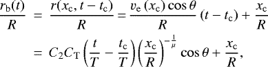
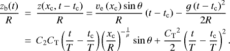
We set here the cylindrical coordinate system where the origin is located at the impact point, r is the horizontal distance from the origin, and the direction of the z-axis is upward (Fig. 1). The position of  of each particle launched at the horizontal distance x is simply given by the ballistic equations as
 (4)
(4)
 (5)
(5)
where we use Eqs. (1) and (3) to obtain the final form of the right-hand side of the two equations.
The ejecta particles following the first ejecta particles are assumed to pile up behind the front surface of the ejecta curtain (the back surface of the curtain is also modeled; see Appendix A). Here we assume a cylindrical symmetry of the ejecta curtain; specifically, the ejecta particles are launched in the same manner regardless of azimuthal direction, although the actual ejecta curtain of the SCI crater was asymmetric (Arakawa et al. 2020). As Arakawa et al. (2020) discusses, the asymmetry of the actual ejecta curtain was most likely produced by the influence of the existing large boulders or the heterogeneity of the subsurface layer, but the excavation flow in each azimuthal direction should be independent of each other in the framework of the Z-model (Maxwell 1977). The particle size and its distribution determine the amount of piled up ejecta particles at any time and position of the ejecta curtain, which directly contribute to the optical depth of the ejecta curtain and enable us to compare our model with the observational results. In this paper we consider two types of particle size distribution: monodisperse and power-law. We describe each case in the following subsections.
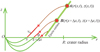 |
Fig. 1 Cross-sectional view of an ejecta curtain and a schematic illustration of ejected particles, constructed according to the theoretical model in cylindrical coordinates (r, z). Particles move along the streaming lines, and are then ejected from the surface at a velocity of ve (x) at an angle of θ. Particles ejected from (x, 0) and (x +Δx, 0) at the time of impact reach points A and B at time t, composing the front surface of the ejecta curtain. |
2.1 Monodisperse ejecta particles
The volume of a subsurface layer including pores that is launched through the surface between r = x and x + Δx piles up onto the front surface defined by azimuthal sweeping of the line connecting point A(r(x, t), z(x, t)) and point B(r(x + Δx, t), z(x + Δx, t)) (see Fig. 1). The volume is defined as VAB, and is calculated using Eq. (2):
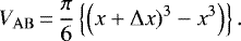 (6)
(6)
The surface area SAB is calculatedas (see Appendix B for derivation)
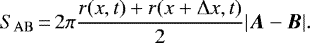 (7)
(7)
Here we consider identical spherical particles with radius am in the ejecta curtain. The total number NAB of the ejecta particles piled up on the area SAB is given by
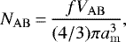 (8)
(8)
where f is the volume filling factor of the subsurface layer (i.e., the volume fraction filled with particles) and assumed to be 0.6, a value for the random close packing. The geometrical coverage (or areal density) τAB of the particles in the corresponding part of the ejecta curtain is then given by
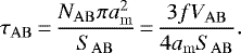 (9)
(9)
Since the ejecta particles are estimated to be larger than ~1 mm as shown later, τAB is almost equivalent to the optical thickness of the ejecta curtain. Then using Eqs. (4), (5), and (9), with changing t and x, we obtain amodel of the time and spatial evolution of an ejecta curtain with a distribution of τ, as shown in Fig. 2. Figure 2 shows two examples of the cross sections of the time and spatial evolution of the ejecta curtain where the border of τ = 1 is indicated. The thickest part of the curtain is the root of the curtain and τ monotonically decreases with increasing height in the curtain. Equation (9) shows that the smaller the constituent particles are, the longer the optically thicker part of the ejecta curtain becomes. This is also shown by comparing the two panels of Fig. 2, where the part of τ > 1 (in red) in the left panel with am = 1 mm is larger than that in the right panel with am = 1 cm.
2.2 Power-law size distribution of ejecta particles
We consider a power-law size distribution for ejecta particles because the size distribution of boulders on Ryugu roughly obeys a power law (Sugita et al. 2019; Michikami et al. 2019). The differential number density of the particles with a range of radius from a to a + d a is given by
 (10)
(10)
where K is a proportionality constant and b is the power-law exponent.
For boulders on Ryugu, various values of b are reported: 3.5–4 (boulder size > 10 m; Sugita et al. 2019), 3.2 (>0.2 m, inside the SCI crater; Arakawa et al. 2020), 3.65 ± 0.05 (> 5 m; Michikami et al. 2019), 2.65 ± 0.05 to 3.01 ± 0.06 (< 4 m; Michikami et al. 2019). We note that these are originally given by cumulative size distributions so the above values are those converted into differential distribution. Taking this variation of b for boulders into account, it is reasonable to assume that the value of b for the ejecta particles lies in the range of 3 to4. The coefficient K is given by solving the equation
 (11)
(11)
where amax and amin are the maximum and the minimum of particle radius a. SubstitutingEq. (10) into Eq. (11), we obtain
 (12)
(12)
Similar to the case of the monodisperse distribution, τAB is calculated as
 (13)
(13)
Substituting Eqs. (10) and (12) into (13), we obtain
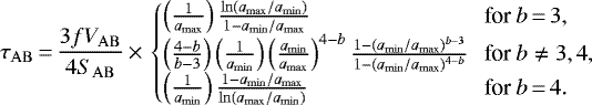 (14)
(14)
This equation indicates that τAB is determined mainly by the maximum size of the particles for the case of b ≤ 3, and by the minimum size for b ≥ 4. In other words, amin can be omitted if we adopt b < ~3, and amax can be dropped if we adopt b > ~4. As a special case, b = 3.5, τAB is given by using the geometrical mean of amax and amin:
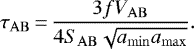 (15)
(15)
Figure 3 shows an example of the time and spatial evolution of an ejecta curtain with a power-law size distribution of ejecta particles.
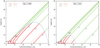 |
Fig. 2 Examples of the evolution model of the ejecta curtain produced by the impact of SCI projectile. Shown is the half cross-sectional view of the ejecta curtain at each time t = 0.01T, 0.1T, 0.5T, 1T, 2T, 3T, where T is the crater formation time. The thick red lines and green dotted lines indicate the front line (area) of the curtain at each time with τ > 1 and τ < 1, respectively.The thin lines indicate the back lines (area) of the curtain. The blue dotted line indicates the trace of the border of τ = 1. The constituent ejecta particles are assumed to have an equal radius am; am = 1 mm (left) and 1 cm (right), respectively. The ejection angle is assumed to be 45 deg. |
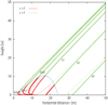 |
Fig. 3 Same as Fig. 2, but the size distribution of the constituent ejecta particles is given by a power law with b = 3.2, amin = 100 μm, and amax = 10 cm. |
3 Measurement of DCAM3 images
The DCAM3 system was equipped with two cameras. One, called DCAM3-A, is designed to monitor impact events during SCI operation which takes low-resolution color images and transmits them via analog signals in real-time to the Hayabusa2 mothership. The other, called DCAM3-D, is for scientific use; it takes high-resolution panchromatic images and transmits them via digital signals in delayed-time to Hayabusa2. In this study we use DCAM3-D images of the ejecta curtain. The details of the specification and the operation plan of DCAM3-D are described in Ogawa et al. (2017) and Ishibashi et al. (2017). DCAM3-D has a wide field of view (FOV: 74 deg × 74 deg) and bright optics (F value = 1.7). The sensor of DCAM3-D is a CMOS image sensor of 2000 × 2000 pix with 8 bit, and takes panchromatic images with a wide wavelength range of 450–850 nm. The pixel resolution is 0.65 mrad pix−1. Since DCAM3 was located about 1 km from the impact point at the time of the impact, the spatial resolution of DCAM3-D is estimated to be less than 1 m pix−1 (and will be determined after the precise orbit of DCAM3 is fixed). The DCAM3-D images were taken at 1 frame per second at maximum for more than 1 h including the time of SCI impact. We can identify faint profiles of the ejecta curtain even in the image taken at 500 s after the impact (Arakawa et al. 2020; Kadono et al. 2020). We note that not all of DCAM3-D images include the ejecta curtain because DCAM3 itself rotated with a little nutation and the ejecta curtain was often moved outside of FOV due to the nutation of DCAM3 (Arakawa et al. 2020; Kadono et al. 2020).
We measured the height of the optically thick part of the ejecta curtain facing DCAM3 in DCAM3-D images that includeclearly the ejecta curtain (Fig. 4). We note that our investigation does not focus on the rim part of the curtain, which geometrically becomes optically thick, even though Fig. 4might give the opposite impression. The height of the optically thick part is compared to that of the part of τ > 1 in the ejecta curtain model we constructed. The correct definition of the position of τ = 1 is the region through which the intensityis reduced to e−1, but it is a bit tricky to determine the height of the optically thick part (τ > 1) from the images. In this study we visually judged the maximum height of the dark (shadow) part as a lower limit of τ = 1 part and the minimum height of the part we determined to see through the far side of DCAM3 as an upper limit.
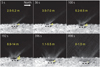 |
Fig. 4 DCAM3-D images of the ejecta curtain. Time (in seconds) after the impact is shown in each panel. The yellow bars indicate the minimum and the maximum heights of the optically thick part of the ejecta curtain, the range of which is also indicated in each image. Modified from Arakawa et al. (2020). |
4 Comparison between the model and the measurement
We compare the model and the observation on the temporal and spatial evolution of the ejecta curtain, focusing on the height of the optically thick part (τ = 1). Then we estimate the ejecta particle size that explains the observation.
4.1 Monodisperse case
Figure 5 shows the model-predicted time evolution of the height of τ = 1 in the ejecta curtain with three different particle sizes (am = 1 mm, 1 cm, and 10 cm) and three different ejection angles (θ = 30, 45, and 60 deg). These lines are clearly distinguishable from each other, suggesting that we can find a unique solution to the particle size. Plotting the measurement data on these lines, we find that the data best fit the case of am = 1 cm among these three cases of the particle size. It is therefore reasonable to assume that the ejecta particles are approximately centimeter-sized if the particles are monodisperse.
The difference in the ejection angle does not strongly affect the estimation of the ejecta particle size, especially in the most likely case of am = 1 cm.
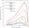 |
Fig. 5 Comparison of the temporal change in the height of the border part of τ = 1 in the ejecta curtain model of the monodisperse particle cases with the measurement data. The line colors (red, green, and blue) correspond to the cases with an ejecta particle size of am = 1 mm, 1 cm, and 10 cm, respectively. The thickness of the lines corresponds to the cases with an ejection angle of θ = 60, 45, and 30 deg. The scatter of the model lines comes from the discreteness of the numerical calculation, which moves the position of τ = 1 as slightly as shown. |
4.2 Power-law distribution case
In Fig. 6, we plot the time evolution curves derived from our models with changing parameters: b (= 4.0, 3.5, 3.2, 3.0), amin (= 0.1, 1 mm), and amax (= 1, 10, 20, 50 cm). Here we fix the ejection angle to 45 deg because the effect of the ejection angle is small, as shown in the monodisperse cases. We note that, as described in Sect. 2.2, amin is significant for the cases of b = 4 (red curves), while amax for b = 3.2 and 3.0 (green and yellow curves, respectively). Plotting the measurement data on this figure, a trend appears: models withrelatively large particles can explain the measurement, although model curves with different b values overlap. Dependent on the value of b, we are able to put a constraint on amin and/or amax as follows. For the case of b = 4 the results suggest amin > 1 mm, while for the cases of b = 3.2 and 3.0 the reasonable value of amax is in the range of 10 to 50 cm (the fraction of the amounts of particles with a size < ~1 mm is lower due to small b). For the case of b = 3.5 the geometrical mean of amin and amax should be greater than 1 mm (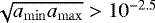 m). As a consequence, given the power-law size distribution, the ejecta particles are typically greater than 1 mm and less than several decimeters even though these are dependent on the power-law index b.
5 Discussion
The ejecta particle size of several centimeters that we estimated on the assumption of the monodisperse distribution is in harmony with the average size using the power-law distribution. Thus, it is reasonable to suppose that the particle size given by assuming the monodisperse distribution is the typical size of the particles. We conclude, therefore, that the size of ejecta particles is typically several centimeters, ranging from ~ 1 mm to several decimeters.
The depth from which the ejecta particles come can be estimated with the Z-model (Maxwell 1977). Given that Z = 3, the deepest depth of the excavation region is theoretically calculated by R∕4, and is ~ 1.8 m for the SCI crater (R = 7.25 m). More conservatively, we calculate the original depth corresponding to the ejecta curtain part of τ = 1 in each model, as shown in Fig. 7. The depth increases with time and is dependent on the parameters; it ranges around 1 m or shallower. Thus, it can be said that our estimated size of the ejecta particles is characteristic of particles in the subsurface layer to the depth of 1 m at least. This implies that the subsurface layer of Ryugu consists of particles of several centimeters in size.
Compared with many boulders greater than 1 m on the uppermost layer of Ryugu (Sugita et al. 2019), smaller particles dominate the subsurface layer. This is consistent with the fact that small boulders are dominant inside the SCI crater (Arakawa et al. 2020). There are some models of surface processes explaining that the subsurface layer consists of small particles (Kadono et al. 2020). On the other hand, our results suggest that the particle size in the subsurface layer (> 1 mm) is not small compared to that on the surfaces of other small bodies, for example Itokawa. We seek a plausible explanation for the lack of minute particles; for example, particles smaller than 1 mm may sink into a deeper region by seismic shaking or mass wasting (Morota et al. 2020). It may be difficult, however, for small particles less than 1 mm to sink deeper because the resistance due to the interparticle cohesive force for such small particles is larger than the gravitational force acting on the particles on the surface of Ryugu (Hartzell & Scheeres 2011; Kimura et al. 2014). The smaller particles may be levitated by impact process or other kinds of mechanism, and blown away by the solar radiation pressure, but it also seems difficult to levitate smaller particles because of the strong cohesive force (Hartzell & Scheeres 2011; Kimura et al. 2014). Another idea is that small particles had been blown away by the solar radiation pressure at the time of formation of Ryugu. Ryugu is thought to be a rubble pile asteroid, made of reaccreted fragments of a disrupted parent body (Watanabe et al. 2019). Only relatively large fragments (> 1 mm), which are not affected by the solar radiation pressure, could have remained around the original orbit and accreted to form Ryugu, thus we could not find smaller particles. We may be able to verify these hypotheses through the detailed analysis of returned samples of Ryugu by investigating, for example, the amount of small particles that exist on the surface and subsurface layers of Ryugu.
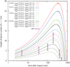 |
Fig. 6 Similar to Fig. 5, but the ejecta curtain is modeled assuming power-law size distributions of ejecta particles. Each color and line type corresponds to b value and amin and amax, as indicated in the legend. |
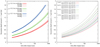 |
Fig. 7 Temporal change of the original depth of the border part of τ = 1 in the modeled ejecta curtains. Shown are the cases for the monodisperse sizes (left) and for the power-law size distributions of ejecta particles (right). Colors and line types are the same as used in Figs. 5 and 6. |
6 Conclusions
The Hayabusa2 mission provided a great opportunity to investigate the subsurface layer of the asteroid Ryugu with using SCI and DCAM3, in other words, excavating subsurface materials and imaging them. We focus on the optical thickness of the ejecta curtain and infer the size of ejecta particles in the curtain emerging from the artificial crater produced by SCI on the surface of Ryugu, comparing a theoretical ejecta curtain model and the DCAM3-D images of the ejecta curtain. As a result, the size of the ejecta particles is estimated to be typically several centimeters, ranging from ~ 1 mm to several decimeters, even though it depends on the model of the particle size distribution. This particle size would reflect the particle size distribution under the surface, especially to a depth of ~ 1 m. This information is a key to understanding the formation and surface evolution of Ryugu and other small Solar System bodies.
Acknowledgements
We are grateful to the reviewer Dr. James Richardson for his helpful comments that greatly improved this paper. We thank all members of the Hayabusa2 team for the successful operation of the SCI and the DCAM3. K.W. and H.K. were supported by the Grants-in-Aid from JSPS (No. 19K03955 and 19H05085).
Appendix A Back surface model of an ejecta curtain
Here we briefly describe how we drew the back surface (line) of the ejecta curtain shown in Figs. 2 and 3. This modeling process was already developed by Richardson et al. (2007), but we used the final apparent crater radius instead of the transient one for the reason described in the main text. In addition, we used the simple scaling laws on the crater formation time and the ejection velocity rather than those used in Richardson et al. (2007). Although our model would be too simple to reconstruct the crater rim morphology, it is effective for the part of the ejecta curtain we focus on.
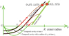 |
Fig. A.1 Schematic illustration of a back surface of an ejecta curtain (cross sectional view). |
The back surface consists of the last particles ejected from the rim of the growing cavity (Fig. A.1). In cylindrical coordinates (r, z), the same as defined in the text, the back surface at the time t(≥ tc), where tc is the formation of the cavity with a radius of xc(≤ R), can be given by the assembly of the positions (rb, zb) of the particles ejected from (xc, 0) at tc, changing tc from 0 to t. The position (rb, zb) is simply given by the following ballistic equations:
 (A.1)
(A.1)
 (A.2)
(A.2)
The relation between tc and xc is given by the following scaling equation on the crater formation time (Holsapple & Housen 2007):
 (A.3)
(A.3)
Plotting (rb, zb) with changing tc from 0 to t, we obtain the back surface of the ejecta curtain.
Appendix B Lateral surface area of a circular truncated cone
As shown in Fig. B.1, we consider two circular cones sharing the same arbitrary opening angle. Their radii of the base circles are denoted Rα and rα (Rα> rα), and the lengths of the conical generatrices are denoted Lc and lc (Lc > lc), respectively. Here, the length of the generatrix of the truncated cone ltc is given by Lc − lc. Let Sc and sc be the lateral surface areas of the bigger and the smaller cones, respectively. Considering the geometric net of the cone as shown in Fig. B.1, Sc and sc are given by
 (B.1)
(B.1)
 (B.2)
(B.2)
The lateral surface area of the truncated cone Atc is defined as
 (B.3)
(B.3)
Substituting Eqs. (B.1) and (B.2) into (B.3), and using the relation Lc = lc + ltc, we obtain
 (B.4)
(B.4)
From a similarity between the two cones, we have
 (B.5)
(B.5)
Substituting this relation into Eq. (B.4), and using Lc = ltc + lc, we have
 (B.6)
(B.6)
This is the same as Eq. (7) in the text. It can also be derived using the general formula for the surface area of a rotating object.
 |
Fig. B.1 Left: schematic illustration of a big and a small circular cone sharing the same opening angle. Right: geometric net of the big cone. |
References
- Arakawa, M., Wada, K., Saiki, T., et al. 2017, Space Sci. Rev., 208, 187 [Google Scholar]
- Arakawa, M., Saiki, T., Wada, K., et al. 2020, Science, 368, 67 [Google Scholar]
- Grott, M., Knollenberg, J., Mamm, M., et al. 2019, Nat. Astron., 3, 971 [Google Scholar]
- Hartzell, C. M., & Scheeres, D. J. 2011, Planet. Space Sci., 59, 1758 [Google Scholar]
- Holsapple, K. A., & Housen, K. R. 2007, Icarus, 187, 345 [Google Scholar]
- Housen, K. R., & Holsapple, K. A. 2011, Icarus, 211, 856 [Google Scholar]
- Housen, K. R., Schmidt, R. M., & Holsapple, K. A. 1983, J. Geophys. Res., 88, 2485 [Google Scholar]
- Ishibashi, K., Shirai, K., Ogawa, K., et al. 2017, Space Sci. Rev., 208, 213 [Google Scholar]
- Kadono, T., Arakawa, M., Honda, R., et al. 2020, ApJ, 899, L22 [Google Scholar]
- Kimura, H., Senshu, H., & Wada, K. 2014, Planet. Space Sci., 100, 64 [Google Scholar]
- McKay, D. S., Heiken, G., Basu, A., et al. 1991, in Lunar Sourcebook, eds. G. H. Heiken, D. T. Vaniman, & B. M. French (Cambridge: Cambridge University Press), 285 [Google Scholar]
- Maxwell, D. E. 1977, in Impact and Explosion Cratering. Planetary and Terrestrial Implications, eds. D. J. Roddy, R. O. Pepin, & R. B. Merrill (New York: Pergamon Press), 1003 [Google Scholar]
- Melosh, H. J. 1989, Impact Cratering: A Geologic Process (New York: Oxford University Press) [Google Scholar]
- Michikami, T., Honda, C., Miyamoto, H., et al. 2019, Icarus, 331, 179 [Google Scholar]
- Morota, T., Sugita, S., Cho, Y., et al. 2020, Science, 368, 654 [Google Scholar]
- Ogawa, K., Shirai, K., Sawada, H., et al. 2017, Space Sci. Rev., 208, 125 [Google Scholar]
- Okada, T., Fukuhara, T., Tanaka, S., et al. 2020, Nature, 579, 518 [Google Scholar]
- Richardson, J.E. 2011, J. Geophys. Res., 116, E12004 [Google Scholar]
- Richardson, E. J., Melosh, H. J., Lisse, C. M., & Carcich, B. 2007, Icarus, 190, 357 [Google Scholar]
- Saiki, T., Imamura, H., Arakawa, M., et al. 2017, Space Sci. Rev., 208, 165 [Google Scholar]
- Sugita, S., Honda, R., Morota, T., et al. 2019, Science, 364, 252 [Google Scholar]
- Tsuchiyama, A., Usesugi, M., Matsushima, T., et al. 2011, Science, 333, 1125 [Google Scholar]
- Watanabe, S., Hirabayashi, M., Hirata, N., et al. 2019, Science, 364, 268 [NASA ADS] [Google Scholar]
- Yano, H., Kubota, T., Miyamoto, H., et al. 2006, Science, 312, 1350 [Google Scholar]
All Figures
|
Fig. 1 Cross-sectional view of an ejecta curtain and a schematic illustration of ejected particles, constructed according to the theoretical model in cylindrical coordinates (r, z). Particles move along the streaming lines, and are then ejected from the surface at a velocity of ve (x) at an angle of θ. Particles ejected from (x, 0) and (x +Δx, 0) at the time of impact reach points A and B at time t, composing the front surface of the ejecta curtain. |
| In the text | |
|
Fig. 2 Examples of the evolution model of the ejecta curtain produced by the impact of SCI projectile. Shown is the half cross-sectional view of the ejecta curtain at each time t = 0.01T, 0.1T, 0.5T, 1T, 2T, 3T, where T is the crater formation time. The thick red lines and green dotted lines indicate the front line (area) of the curtain at each time with τ > 1 and τ < 1, respectively.The thin lines indicate the back lines (area) of the curtain. The blue dotted line indicates the trace of the border of τ = 1. The constituent ejecta particles are assumed to have an equal radius am; am = 1 mm (left) and 1 cm (right), respectively. The ejection angle is assumed to be 45 deg. |
| In the text | |
|
Fig. 3 Same as Fig. 2, but the size distribution of the constituent ejecta particles is given by a power law with b = 3.2, amin = 100 μm, and amax = 10 cm. |
| In the text | |
|
Fig. 4 DCAM3-D images of the ejecta curtain. Time (in seconds) after the impact is shown in each panel. The yellow bars indicate the minimum and the maximum heights of the optically thick part of the ejecta curtain, the range of which is also indicated in each image. Modified from Arakawa et al. (2020). |
| In the text | |
|
Fig. 5 Comparison of the temporal change in the height of the border part of τ = 1 in the ejecta curtain model of the monodisperse particle cases with the measurement data. The line colors (red, green, and blue) correspond to the cases with an ejecta particle size of am = 1 mm, 1 cm, and 10 cm, respectively. The thickness of the lines corresponds to the cases with an ejection angle of θ = 60, 45, and 30 deg. The scatter of the model lines comes from the discreteness of the numerical calculation, which moves the position of τ = 1 as slightly as shown. |
| In the text | |
|
Fig. 6 Similar to Fig. 5, but the ejecta curtain is modeled assuming power-law size distributions of ejecta particles. Each color and line type corresponds to b value and amin and amax, as indicated in the legend. |
| In the text | |
|
Fig. 7 Temporal change of the original depth of the border part of τ = 1 in the modeled ejecta curtains. Shown are the cases for the monodisperse sizes (left) and for the power-law size distributions of ejecta particles (right). Colors and line types are the same as used in Figs. 5 and 6. |
| In the text | |
|
Fig. A.1 Schematic illustration of a back surface of an ejecta curtain (cross sectional view). |
| In the text | |
|
Fig. B.1 Left: schematic illustration of a big and a small circular cone sharing the same opening angle. Right: geometric net of the big cone. |
| In the text | |
Current usage metrics show cumulative count of Article Views (full-text article views including HTML views, PDF and ePub downloads, according to the available data) and Abstracts Views on Vision4Press platform.
Data correspond to usage on the plateform after 2015. The current usage metrics is available 48-96 hours after online publication and is updated daily on week days.
Initial download of the metrics may take a while.