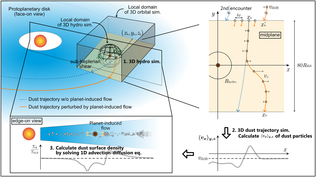
Schematic illustration of our model. We performed 3D hydrodynamical simulations on the spherical polar grid (the black sphere), which hosts a planet located at its center (the brown-filled circle; Sect. 2.3). We consider the planet on a fixed circular orbit with the orbital radius, a. We adopt unperturbed sub-Keplerian shear flow at the outer boundary of the hydrodynamical simulations (the green arrows). We then calculated the trajectories of particles influenced by the planet-induced gas flow in the frame co-rotating with the planet (the local box; Sect. 2.4.1). We used the limited part of the computational domain of hydrodynamical simulation, R_hydro, in orbital calculations of dust particles (Sect. 2.4.1). The x and z coordinates of the starting point of particles, x_s and z_s, are the parameters. The starting point of orbital calculation is beyond R_hydro. The spatial interval of orbital calculation in the x direction is δx (Sect. 2.4.2). The x coordinate of the particle at the edge of the domain of orbital calculation is x_e. The x coordinate of the particle after one synodical orbit, x′_S, is given by Eq. (27) (Sect. 3.3). The schematic trajectories of particles are shown by the dashed blue lines (without the influence of planet-induced gas flow) and solid orange lines (perturbed by the planet-induced gas flow). The open circles on the trajectory correspond to the position of a particle at specific time intervals, ∆t(v_y,0, z_s) (Eq. (10)). The black arrows on the trajectories are the velocities in the x direction of a particle at each position, v_x. It should be noted that we do not follow trajectories outside the calculation domain of orbital calculations. Instead, we assumed the uniform and Gaussian distributions of dust particles in the azimuthal and vertical directions outside the local domain of orbital calculation, respectively, where the particles have a fixed velocity in the x direction, v_drift. Based on the obtained spatial distribution of dust in the global domain, we calculated the azimuthally and vertically averaged drift velocity, 〈v_x〉_y,z (Eq. (17)). Finally, we calculated the dust surface density by incorporating 〈v_x〉_yz into the 1D advection-diffusion equation (Eq. (20)).